E
S
E
A
R
C
H
R
E
P
R
O
R
I
D
I
A
P
Rue du Simplon 4IDIAP Research Institute
1920 Martigny − Switzerland www.idiap.ch Tel: +41 27 721 77 11 Email: [email protected]
P.O. Box 592 Fax: +41 27 721 77 12
The more you learn, the less
you store:
memory-controlled
incremental support vector
machines
Andrzej Pronobis
aBarbara Caputo
b cIDIAP–RR 06-51
September 2006
submitted for publication
a NADA/CAS, KTH, Sweden [email protected] b IDIAP - [email protected]
The more you learn, the less you store:
memory-controlled incremental support vector
machines
Andrzej Pronobis
Barbara Caputo
September 2006 submitted for publication
Abstract. The capability to learn from experience is a key property for a visual recognition algorithm working in realistic settings. This paper presents an SVM-based algorithm, capable of learning model representations incrementally while keeping under control memory requirements. We combine an incremental extension of SVMs [1] with a method reducing the number of support vectors needed to build the decision function without any loss in performance [2], introducing a parameter which permits a user-set trade-off between performance and memory. The resulting algorithm is guaranteed to achieve the same recognition results as the original incremental method while reducing the memory growth. Moreover, experiments in two domains of material and place recognition show the possibility of a consistent reduction of memory requirements with only a moderate loss in performance. For example, results show that when the user accepts a reduction in recognition rate of 5%, this yields a memory reduction of up to 50%.
1
Introduction
Basic visual operations such as categorization and complex tasks such as scene interpretation have long been major challenges in computer vision. A system able to perform these tasks should include facilities for understanding and learning, where understanding here means both recognition and categorization of objects and scenes. A system with a realistic complexity cannot be engineered: this calls for methods for automatic acquisition of models and representations allowing the system to work in an open-ended fashion, i.e. beyond initial specification. A highly desirable property for a visual recognition algorithm working in realistic settings is the capability to learn from experience and update incrementally its internal representation. The possibility to learn continuously is particularly important for all those applications where, in spite of a vast batch training set and unlimited training time, it is impossible to provide a database which will remain representative of the modeled visual class during time. For instance, some visual categories like phones or computers have grown dramatically over the last 20 years. New category members like cell phones and laptops have appeared, changing our visual models of these categories. Another example is indoor place recognition, where the variability of a room’s appearance is so high (people using the room, furniture relocated or changed, objects being taken out of drawers, illumination changes and so forth) that is virtually impossible to collect a training database covering all these possibilities.
Discriminative methods have become widely popular for visual recognition, achieving impressive results on several applications [3, 4, 5, 6]. Within discriminative classifiers, SVM techniques provide powerful tools for learning models with good generalization capabilities; in some domains like object and material categorization, SVM-based algorithms are state of the art [7, 8]. This makes it worth to investigate whether it is possible to perform continuous learning with this type of methods. Several incremental extensions of SVMs have been proposed in the machine learning community [9, 10, 1, 11, 12]. Between these methods, the approximate techniques [9, 11, 1] seem better suited for visual recognition because, at each incremental step, they discard non-informative training vectors, thus reducing the memory requirements. Other methods, such as [10], instead require to store in memory all the training data, eventually leading to a memory explosion; this makes them unfit for continuous learning of visual patterns.
This paper presents an SVM-based incremental method which performs like the batch algorithm while reducing the memory requirements. We combine an approximate technique for incre-mental SVM [1] with an exact method that reduces the number of support vectors needed to build the decision function without any loss in performance [2]. This results in an algorithm performing as the original incremental method with a reduction in the memory requirements. We then present an extension of the method for the exact simplification of the support vector solution [2]. We introduce a parameter that links SVM’s performance to the amount of vectors that is possible to discard. This allows a user-set trade-off between performance and memory reduction. The algorithms were tested in two domains, material categorization and indoor place recognition, using several descriptors and kernel types. For this last application, we recorded a new database in our laboratory which images office environments across a time-range of three months, thus capturing the natural variability of rooms. In summary, the contributions of this paper are:
• We implemented and tested the fixed-partition incremental SVM [1] and benchmarked it against the batch algorithm. Results show that their performance is statistically equivalent, but the incremental method does not consistently achieve a memory reduction compared to the batch model.
• We implemented and tested a method for the exact simplification of the support vector solution [2]. The algorithm was further extended by introducing a parameter, to be set by the user, which allows a trade-off between performance and memory. Although our interest here was in combining these algorithms with incremental SVM, these methods can be used for any SVM-based classification algorithm.
• We combined these algorithms obtaining a new incremental SVM with a mechanism for memory control. At each incremental step the number of support vectors to be stored can be reduced, depending on the application, (a) without any loss in performance, or (b) with a controlled decrease in recognition rate which yields a consistent memory reduction. Experiments show that in the case(a)the algorithm achieves a reduction on the number of stored support vectors of 32%. In the case(b), results show that when it is acceptable a reduction in recognition rate of 5%, this yields a reduction of 50% in the number of stored support vectors.
• We built a new database for indoor place recognition. It consists of several sets of pictures taken in five rooms of different functionality, under various conditions. We placed a special emphasis on capturing the variability of the environments, and we imaged each room under many viewpoints and angles, across a range of time of several months. Because of the high resolution of the images (1024×768 pixels), the database can be used for testing scene recognition systems, context-based object recognition methods and visual attention algorithms.
The paper is organized as follows: after a review of the existing literature (section 2), section 3 describes the databases and relative feature types used throughout the paper. Section 4 reviews approximate techniques for incremental SVM and presents an experimental evaluation of one of these methods. Section 5 describes the memory reduction algorithms and evaluates their performance for different kernel types. Section 6 presents our memory-controlled incremental SVM and shows its effectiveness with a set of experiments. The paper concludes with a summary discussion and possible directions for future work.
2
Related Work
In the recent years, the need for continuous and incremental learning methods is becoming more and more acknowledged. This stimulated the research in the machine learning community directed towards developing extensions for algorithms that were commonly used due to their superior performance but were missing the ability to be trained incrementally. As a result, methods such as Incremental PCA have been invented and successfully applied e.g. for mobile robot localization [13, 14]. As it was already mentioned, several incremental extensions have been introduced also for Support Vector Machines [9, 10, 1, 11, 12]. However, the results of experiments that can be found in the literature do not give a clear answer if it is possible to apply them for complex real-world problems such as e.g. scene recognition. The question how to maintain the complexity of a continuously trained classifier also remained unanswered. At the same time, several methods have been proposed that allow to reduce the complexity of SVM solutions and make it more suitable for large-scale problems [2, 15, 16, 17, 18]. However, to the knowledge of the authors, non of them has so far been tried in the incremental learning scheme.
3
Experimental Setup
In this section we describe the databases and the feature types used in this paper. For the experiments on material categorization we used a database recently presented [7] and state of the art descriptors [19] (section 3.1). For the experiments on indoor place recognition, we present a new database which captures the variability of five different rooms in a working environment across a span of time of three months (section 3.2). Previous work on scene recognition makes use of global descriptors [20] as well as local features [21]. In order to asses the difficulty of the database, we used two feature types: a rich global descriptor [22] and SIFT features [23].
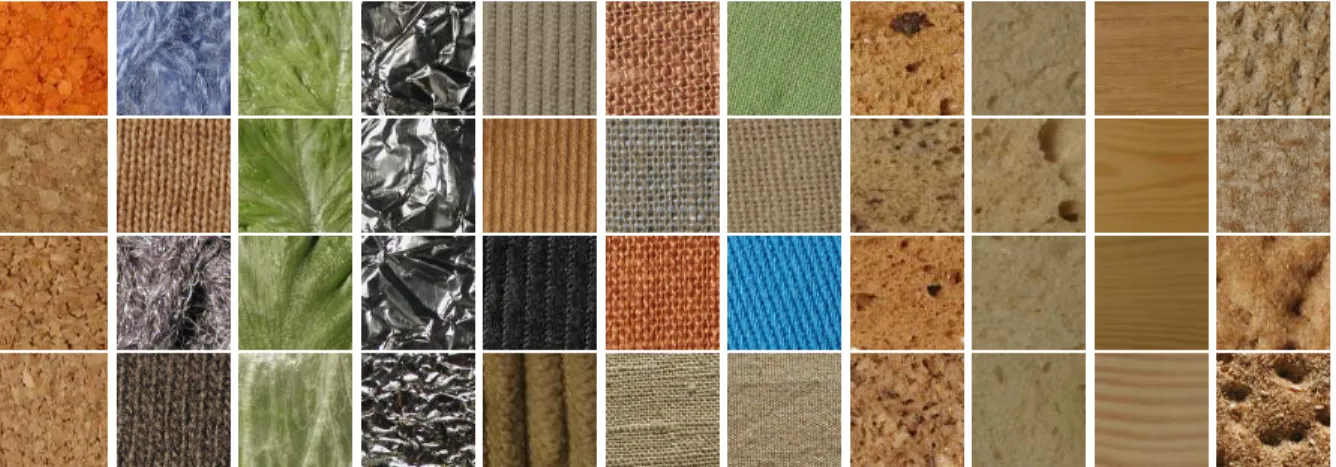
Figure 1: The variations within each category of the TIPS2 database. Each row shows one example image from each of four samples of a category. In addition, each sample was imaged under varying pose, illumination and scale conditions.
3.1
Material Categorization
We performed the material categorization experiments on the TIPS2 database, which contains 4 planar samples of each of 11 materials ([7], Fig 1). Many of these materials have 3D structure, implying that their appearance can change considerably as pose and lighting are changed. TIPS2 contains images at 9 scales equally spaced logarithmically over two octaves. At each scale, materials were imaged under 3 poses (frontal, rotated 22.5◦ left and 22.5◦ right) and 4 illumination conditions (frontal, 45◦
from the top and 45◦ from the side, all taken with a desk-lamp with a Tungsten light bulb; the
fourth illumination condition consisted of the fluorescent lights in the laboratory). In total there are 9×3×4 = 108 images per sample. As descriptors we used the rotationally invariant MR8 [19] which has shown good performances on this database [7].
3.2
Place Recognition
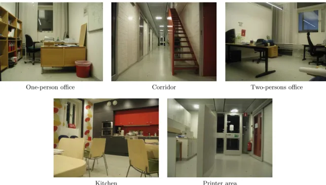
We performed the place recognition experiments on the INDECS database (INDoor Environment under Changing conditionS) [24], a new database which represents one of the contributions of this paper. The database consists of 5 different rooms (a one-person office, a two-persons office, a kitchen, a corridor and a printer area) imaged under different viewpoints and locations. Images were acquired using an Olympus C-3030ZOOM digital camera mounted on a tripod. The height of the tripod was constant and equal to 76 cm; all images were acquired with a resolution of 1024×768 pixels, with the flesh disabled, the zoom set to wide-angle mode and the auto-focus enabled. Fig 2 shows examples of the images recorded. For each room, images were taken at different times of the day and with different weather conditions (sunny, cloudy and night), across a span of time of three months. In this way, we captured the visual variability of each room under different illumination conditions and we recorded the normal activities in the rooms (presence/absence of people, furniture relocated, changed, added or removed). Fig 3 shows some examples of these types of variability for some rooms. We marked out in each room several points (approximately one meter from each other) where we positioned the camera for each acquisition. The number of points changed with the dimension of the room and goes from a minimum of 9 for the one-person office to a maximum of 32 for the corridor. At each location we took 12 pictures, one every 30◦. In total there are 3264 images (324 for the one-person office, 492
for the two-persons office, 648 each for the kitchen and the printer area, and 1152 for the corridor). Experiments were conducted using SIFT features [23] as local descriptors and Composed Receptive Fields Histograms (CRFH, [22]) as global features. For this last feature type, we tested several different combinations of receptive fields in a set of preliminary experiments. Based on the results we obtained,
One-person office Corridor Two-persons office
Kitchen Printer area
Figure 2: Some examples from the INDECS database
we decided to use CRFH computed from second order normalized Gaussian derivative filters, at two different scales, throughout the paper.
4
Incremental SVM
This section presents the incremental SVM technique that will be one of the building blocks of our memory-controlled algorithm. After a brief review of the theory behind this type of algorithms (section 4.1), the remaining of the section describes the approximate technique used in this paper (section 4.2) and presents an experimental evaluation of its performance against the batch method (section 4.3).
4.1
SVM: the batch algorithm
Support Vector Machines (SVMs, [25, 26]) belong to the class of large margin classifiers. Consider the problem of separating the set of training data (x1, y1), . . .(xm, ym), wherexi∈ ℜN is a feature vector
andyi∈ {−1,+1}its class label. If we assume that the two classes can be separated by an hyperplane
w·x+b= 0, the optimal hyperplane is the one which has maximum distance to the closest points in the training set. The optimal values forwandb can be found by solving a constrained minimization problem, which results in a classification function
f(x) = sgn m X i=1 αiyiw·x+b ! , (1)
whereαi andbare found by using an SVC learning algorithm [25, 26]. Most of theαi’s take the value
of zero; thosexiwith nonzeroαi are the “support vectors”. It can be seen from eq. 1 that the speed
of classification as well as the memory required to store a trained model are directly proportional to the number of support vectors. The extension to multiclass can be done following several strategies [26, 25]; here we used the pairwise approach [26, 25]. To obtain a nonlinear classifier, one maps the data from the input space ℜN to a high dimensional feature space Hby x→Φ(x)∈ H, such that
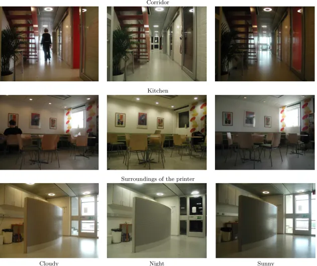
Corridor
Kitchen
Surroundings of the printer
Cloudy Night Sunny
Figure 3: Examples of pictures from the INDECS database, taken under three different illumination and weather conditions for some rooms.
the mapped data points of the two classes are linearly separable in the feature space. Assuming there exists a kernel functionK such that K(x,y) = Φ(x)·Φ(y), then a nonlinear SVM can be construct by replacing the inner productx·yin the linear SVM by the kernel functionK(x,y)
f(x) = sgn m X i=1 αiyiK(xi,x) +b ! (2)
This corresponds to constructing an optimal separating hyperplane in the feature space. In this paper we will use the folowing kernel functions:
• polynomial:K(x,y) = (x·y+ 1)d,
• RBF (Gaussian): K(x,y) = exp{−γ||x−y||2},
• χ2: K(x,y) = exp{−γχ2(x,y)},
4.2
SVM: an Incremental Extension
Among all incremental SVM extensions proposed in the machine learning literature so far [1, 9, 28, 10], approximate methods seem to be the most suitable for visual recognition: firstly - as opposed to exact methods like [10]- they discard a significant amount of the training data at each incremental step. Secondly, they are expected to achieve performances not too far from those obtained by an SVM trained on the complete data set (batch algorithm), because at each incremental step the algorithm remembers the essential class boundary information regarding the data seen so far (in form of support vectors). This information contributes properly to generate the classifier at the next iteration.
Once a new batch of data is loaded into memory, there are different possibilities for the updating of the current model, which might discard a part of the new data according to some fixed criteria [9, 1]. In this paper we use the fixed-partition technique, which was introduced first in [1]. In this method the training data set is partitioned in batches of fixed sizek:
T ={(x1, y1), . . . ,(xm, ym)}={T1,T2, . . .Tn}, with Ti={(xij, y i j)} k j=1.
At the first step, the model is trained on the first batch of dataT1, obtaining a classification function
f1(x) = sgn m1 X i=1 α1iy 1 ix 1 i ·x+b 1 ! .
At the second step, a new batch of data is loaded into memory; then, thenew training set becomes Tinc2 ={T2∪SV1}, SV1={(x1i, y
1
i)} m1 i=1,
whereSV1are the support vectors learned at the first step. The new classification function will be:
f2(x) = sgn m2 X i=1 α2iy 2 ix 2 i ·x+b 2 ! .
Thus, as new batches of data points are loaded into memory, the existing support vector model is updated, so to generate the classifier at that incremental step. Note that this incremental method can be seen as an approximation of the chunking technique used for training SVM [25]. Indeed, the chunking algorithm is an exact decomposition which iterates through the training set to select the support vectors. The fixed-partition incremental method instead scan through the training data just once, and once discarded, does not consider them anymore. The fixed-partition incremental algorithm has been tested on several benchmark databases commonly used in the machine learning community [9] and on a simple optical character recognition problem [28], obtaining good performances compared to the batch algorithm and other approximate methods.
4.3
Experimental Evaluation
We performed two sets of experiments to evaluate the fixed-partition incremental SVM. The first set was performed on the material categorization database; the second on the place recognition database. For these experiments we employed our extended version of the libsvm [29] software, and we set
C= 100. We used RBF kernel in case of material categorization andχ2(for global features) or local kernel [27] (for local features) in case of place recognition. Kernel parameters were determined via cross-validation.
For the material categorization experiments, we splitted the TIPS2 database in a training and test set, with the training set consisting of three samples per material, and the test set consisting of the remaining fourth sample; as in [7], we considered 4 possible splits. The training set was further
1 2 3 Ste p 4 0 5 0 6 0 7 0 8 0 9 0 C la s s i f ic a t io n ra te ( % ) C la s s ific a t io n ra t e Batch Incre m e nta l 1 2 3 Ste p 2 0 0 4 0 0 6 0 0 8 0 0 1 0 0 0 1 2 0 0 14 0 0 1 6 0 0 No. o fs u p po r tv e c t o r s S t o re d s u p p o rt v e ct o rs Batc h Inc re m e nta l
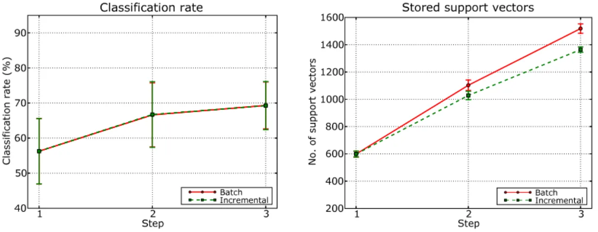
Figure 4: Results on the TIPS2 database using fixed-partition incremental SVM and the batch algo-rithm. The incremental method achieves a memory reduction while obtaining the same performance as batch SVM.
divided in three subsets, each consisting of all the views for one sample per material. Each subset was added to the model during each incremental step. For each partition, we performed experiments on four different orderings of the incremental steps. For instance, for the partition with sample 1, 2, 3 into the training set we ran 4 different experiments considering the incremental sequences (a) 1, 2, 3; (b) 2, 1, 3; (c) 2, 3, 1 (d) 3, 2, 1. Thus, in total we ran 16 different experiments; here we report the averaged results with standard deviations. Fig 4, left, shows the recognition rates obtained, at each step of the incremental update, using the batch SVM on the whole training data and the fixed-partition incremental algorithm. Fig 4, right, shows the number of support vectors stored by both algorithms at each step of the incremental procedure. We see that there is no loss in performance of the incremental algorithm compared to the batch one, while there is a statistically significant reduction of the number of support vectors in the incremental algorithm. It is interesting to observe that the reduction in memory requirements for the incremental algorithm is more pronounced at the third (and last) step, which also corresponds to a less pronounced growth in recognition rate. This might indicate that, for this categorization problem, the statistic relative to each material is already representative at that step, and the incremental procedure acts like a noise filter with respect to the previous incremental steps, actually helping the learning algorithm to find a more compact representation. These results are in agreement with those reported in [9], where only two-class problems were considered.
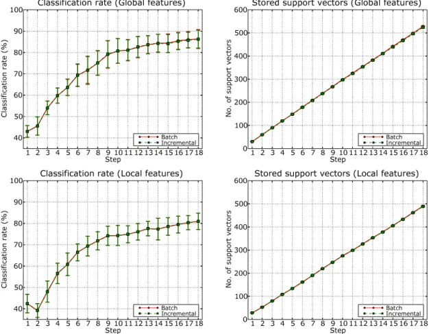
We followed a similar procedure for the place recognition experiments. The INDECS database was partitioned into a training and test set, where the training set consisted of the images acquired under two different weather conditions from 9 locations in each room. The test set consisted of the images of the remaining weather condition acquired from the same 9 locations (6 images per location). We ran experiments on all three possible splittings into training and test set. Within each split, the training set was sub-partitioned into 9 subsets for each weather condition, resulting in 18 incremental batches in total. At every split, we considered two possible orderings for the weather conditions. Thus, in total, we performed six experiments for each of the two feature types. Fig 5 shows the average results obtained using both the CRFH global representation and the SIFT local descriptor. We see that once again incremental and batch SVM obtain the same performance at each incremental step (Fig 5, left), but on this application the incremental method does not achieve any memory reduction compared to the batch algorithm (Fig 5, right). The same behaviour can be observed for both types of features. This might depend on the intrinsic difficulty of the problem: rooms exhibit a considerable variability in their visual appearance, and each incremental subset consists of images taken at different positions in the environments.
1 2 3 4 5 6 7 8 9 1 0 1 1 1 2 1 3 14 1 5 1 6 1 7 1 8 Ste p 4 0 5 0 6 0 7 0 8 0 9 0 1 0 0 C la s s i f ic a t io n ra te ( % ) C la s s ific a t io n ra t e ( G lo b a l fe a t u re s ) Batch Inc re m e nta l 1 2 3 4 5 6 7 8 9 1 0 1 1 1 2 1 3 14 1 5 1 6 1 7 1 8 Ste p 0 1 0 0 2 0 0 3 0 0 4 0 0 5 0 0 6 0 0 No. o fs u p po r tv e c to r s S t o re d s u p p o rt v e ct o rs (G lo b a l fe a t u re s ) Batch Inc re m e nta l 1 2 3 4 5 6 7 8 9 1 0 1 1 1 2 1 3 14 1 5 1 6 1 7 1 8 Ste p 4 0 5 0 6 0 7 0 8 0 9 0 1 0 0 C la s s i fic a t io n ra te ( % ) C la s s ific a tio n ra t e (L o c a l fe a t u re s ) Batch Inc re m e nta l 1 2 3 4 5 6 7 8 9 1 0 1 1 1 2 1 3 14 1 5 1 6 1 7 1 8 Ste p 0 1 0 0 2 0 0 3 0 0 4 0 0 5 0 0 6 0 0 No. o fs u p po r tv e c to r s S t o re d s u p p o rt v e ct o rs ( L o c a l fe a t u r e s ) Batch Inc re m e nta l
Figure 5: Results on the INDECS database using incremental SVM and the batch algorithm, for both global and local features. On this application, in both cases, the two methods have comparable performance and memory requirements.
incremental SVM performs as the batch algorithm. A significant drawback of the method is that it does not guarantee a reduction of the number of stored support vectors. For visual applications like place recognition for topological mapping, this is a serious issue, as it may lead to a memory explosion. In the next section we will present a method for the reduction of the memory requirements of the support vector solution. As it will be shown in section 6, this method, combined with the fixed-partition approach, can be used to design a memory-controlled incremental SVM.
5
Exact Simplification of SVM Solution
Experiments presented in section 4 showed that the fixed-partition incremental SVM can achieve the classification performance of the batch algorithm while using fewer support vectors. While this suggests that the solution found using the standard SVC learning algorithm is not always minimal, experiments presented in [1] showed that rejecting even a small amount of support vectors may cause a strong decrease in performance. This raises the question of whether the complexity of the support vector solution can be reduced while preserving its optimal performance. A possible solution has been proposed by Downset al[2]. Their method reduces the number of support vectors of a trained classifier, eliminating those which can be expressed as a linear combination of the others in the feature space. The weights are updated accordingly, which ensures that the decision function is exactly the
same as the original. This results in a reduction of the complexity of the classifier, without any loss in performance.
The rest of this section is organized as follows: section 5.1 reviews the method presented in [2], gives some details on its implementation and presents an extension of the algorithm that allows the user to trade performance for memory requirements, when necessary. Section 5.2 describes a series of experiments evaluating both methods on our two chosen applications. Although we developed the algorithm having in mind its integration with incremental SVM techniques, it can be used for reduc-ing the memory requirements (as well as speed durreduc-ing recognition) of any SVM-based classification method.
5.1
The Algorithm
The idea behind the algorithm by Downset al [2] is that the set of support vectorsX ={xi}mi=1 is
not guaranteed to be linearly independent. Let us suppose that the firstrsupport vectors are linearly independent, and the remainingm−rdepend linearly on those in the feature space: ∀j =r+ 1, . . . m, xj∈span{xi}ri=1. Then it holds
K(x,xj) = r
X
i=1
cijK(x,xi), (3)
and the classification function (2) can be rewritten as
f(x) = sgn ( r X i=1 αiyiK(x,xi)+ + m X j=r+1 αjyj r X i=1 cijK(x,xi) +b). (4)
If we define the coefficientsγij such that αjyjcij=αiyiγij andγi=Pmj=r+1γij, then eq. (4) can be
written as f(x) = sgn ( r X i=1 αiyiK(x,xi)+ r X i=1 αiyi m X j=r+1 γijK(x,xi) +b) = sgn r X i=1 b αiyiK(x,xi) +b ! (5) where b αi=αi(1 +γi) =αi 1 + m X j=r+1 αjyjcij αiyi . (6)
Thus, the resulting classification function (eq. (5)) requires nowm−r less kernel evaluations than the original one (eq. (2)). In order to find the linearly independent subset of the support vectors and the values of thecij coefficients, we applied the QR factorization algorithm with column pivoting [30]
to the support vector matrix.
Two interesting points can be made on the QR factorization and the column pivoting strategy: first, it allows to reveal the numerical rank of the matrix with respect to a parameterτ, which acts as a threshold in defining the condition of linear dependence. Second, the algorithm performs a permutation of the columns of the matrix such that, if for a given value of τ the rank of the matrix is r, then the linearly independent columns will occupy the firstr positions. Also, these r columns
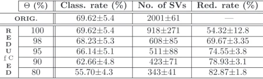
Θ(%) Class. rate (%) No. of SVs Red. rate (%) ORIG. 69.62±5.4 2001±61 — R E D U f ¯C E D 100 69.62±5.4 918±271 54.32±12.8 98 68.23±5.3 608±85 69.67±3.35 95 66.14±5.1 511±88 74.55±3.8 90 62.66±4.8 423±71 78.93±3.1 80 55.70±4.3 343±41 82.87±1.8
Table 1: Average results of the evaluation of the reduction algorithm on the TIPS2 database, for the Gaussian kernel. The Θ parameter denotes a percentage of the original classification rate, that is guaranteed to be preserved after the reduction. The uncertainties are given as one standard deviation.
Θ(%) Class. rate (%) No. of SVs Red. rate (%)
ORIG. 72.28±6.1 1525±36 — R E D U f ¯C E D 100 72.28±6.1 833±340 45.69±21.3 98 70.83±6.0 708±180 53.77±10.9 95 68.67±5.8 606±114 60.38±6.7 90 65.05±5.5 475±80 68.89±4.6 80 57.82±4.9 336±62 78.01±3.7
Table 2: Average results of the evaluation of the reduction algorithm on the TIPS2 database, for the
χ2kernel. The Θ parameter denotes a percentage of the original classification rate, that is guaranteed
to be preserved after the reduction. The uncertainties are given as one standard deviation.
will be ordered according to the degree of their relative linear independence. On the basis of these observations, we propose to consider the threshold τ as a parameter of the algorithm that allows the user to control the number of support vectors to be kept in memory. Clearly, as the value of τ
grows, eq. (5) will become more and more an approximation of the exact solution. Anyway, we want to underline that the informative content of a discarded support vector xj is not completely lost,
as its weight αj is used to compute the updated value of the weights αbi for the remaining support
vectors. This should result in a graceful decrease of classification performance compared to the optimal solution. Thus, the parameter τ can be used as an effective way to trade performance for memory requirements and speed during classification, depending on the task at hand. This extended version of the original algorithm by Downset alcan be seen as an alternative approach to approximate SVM methods like [15, 16, 17].
5.2
Experimental Evaluation
We tested the algorithm with an extensive set of experiments on the TIPS2 and INDECS databases. For each experiment, we first trained the classifier using the standard SMO algorithm. Then, starting from the obtained decision function, we applied the reduction algorithm increasing the value of the
τ parameter, which led to a progressive reduction of the classification rates and of the number of support vectors. Table 1-3 shows the results obtained on the TIPS2 database using three different kernel functions (RBF, χ2, polynomial) for a series of experiments where the training set consisted of 3 samples per material, and the test set consisted of the remaining sample. As in section 4.3, experiments were performed on 4 different partitions and we report here the averaged results; the symbol Θ was used to denote the percentage of the original classification rate that is guaranteed to be preserved after the reduction. Note that, in the experiments presented here, we considered the classification rate of the resulting solution as a constraint on the amount of reduced support vectors. However, depending on the application, the problem may be reformulated to provide the amount
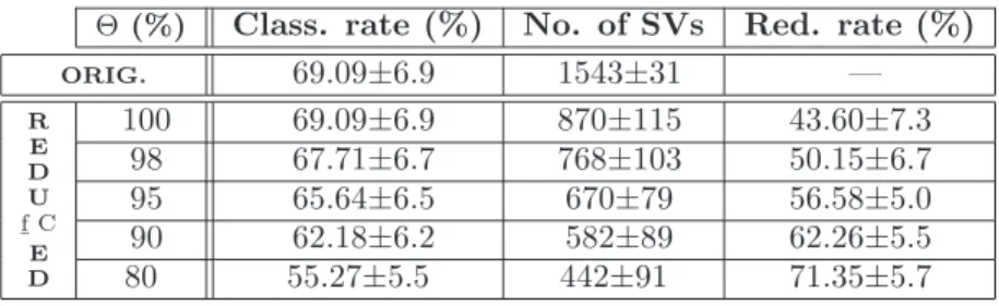
Θ(%) Class. rate (%) No. of SVs Red. rate (%) ORIG. 69.09±6.9 1543±31 — R E D U f ¯C E D 100 69.09±6.9 870±115 43.60±7.3 98 67.71±6.7 768±103 50.15±6.7 95 65.64±6.5 670±79 56.58±5.0 90 62.18±6.2 582±89 62.26±5.5 80 55.27±5.5 442±91 71.35±5.7
Table 3: Average results of the evaluation of the reduction algorithm on the TIPS2 database, for the polynomial kernel. The Θ parameter denotes a percentage of the original classification rate, that is guaranteed to be preserved after the reduction. The uncertainties are given as one standard deviation.
Θ(%) Class. rate (%) No. of SVs Red. rate (%)
ORIG. 75.67±3.89 1000±23 — R E D U f ¯C E D 100 75.67±3.89 990±25 1.04±0.43 98 74.16±3.81 953±31 4.75±0.9 95 71.89±3.69 823±29 17.70±2.01 90 68.11±3.50 677±43 32.33±3.23 80 60.54±3.11 405±28 59.49±1.94
Table 4: Average results of the evaluation of the reduction algorithm on the INDECS database, for the
χkernel. The Θ parameter denotes a percentage of the original classification rate, that is guaranteed to be preserved after the reduction. The uncertainties are given as one standard deviation.
of desired memory reduction. We see that the algorithm achieves a reduction in the number of stored vectors within the range of∼44-54%, depending on the kernel, while keeping the classification rate intact. When the application allows a small loss in performance, memory requirements may be further reduced by exploiting the ability of the algorithm to approximate the solution. Note that the classification rate decreases monotonically with the number of support vectors.
All the results presented in this section were obtained for the pairwise multiclass SVM extension. The experiments were repeated for the one-versus-all method [26, 25], and different number of training samples per material (1 or 2), yielding results consistent with those reported here. It is interesting to observe that the reduction rate in support vectors grows with the dimension of the training set. For instance, the average reduction rate obtained training on one sample per material is ∼44% when it is acceptable a decrease in recognition rate of 5%. This value is considerably lower of the ∼75% in reduction rate obtained under similar conditions, using 3 samples per material during training.
The experiments with the INDECS database were performed in a similar fashion (we report the
Θ(%) Class. rate (%) No. of SVs Red. rate (%)
ORIG. 69.40±3.02 968±14 — R E D U f ¯EC D 100 69.40±3.02 929±45 3.95±3.36 98 68.01±2.96 805±37 16.83±3.73 95 65.93±2.87 662±18 31.54±1.70 90 62.46±2.72 492±51 49.23±4.70 80 55.52±2.42 284±28 70.68±2.75
Table 5: Average results of the evaluation of the reduction algorithm on the INDECS database, for the local kernel. The Θ parameter denotes a percentage of the original classification rate, that is guaranteed to be preserved after the reduction. The uncertainties are given as one standard deviation.
results in Table 4-5). The training sets were formed from all the pictures acquired under one weather condition, while the test sets consisted of the whole images of the remaining weather conditions. The presented results were obtained using both global and local image descriptors and averaged over all three possible splits. Again, the χ2 kernel was used for experiments with composed receptive field
histograms (CRFH), and the local kernel [27] was used in case of local features. We can observe that, while the complexity of the place recognition problem makes the exact simplification method less effective, in both cases, it is still possible to achieve substantial memory reductions by means of approximation. Additionally, this suggests that the algorithm can be successfully applied for non-Mercer kernels [27].
6
Memory-controlled Incremental SVM
The fixed-partition incremental learning algorithm described in section 4 was shown to perform well on different kinds of visual data. However, experiments revealed that at each incremental step the memory requirements can grow considerably. This is a serious limitation for an incremental method aiming to work on real-world applications. In section, 5 we presented a technique for controlling the amount of stored support vectors in a principled way, and we extended it so to obtain an even greater reduction rate when the user accepts a fixed decrease in performance. This is a reasonable assumption, particularly for multi-sensory systems. Our idea is to combine these two algorithms together, obtaining an incremental SVM method with a mechanism for a controlled growth of the memory requirements. We propose to apply the reduction algorithm ateach incremental step. The new representation of the data is then built from the remaining support vectors. We will show through experiments that this approach can successfully control the amount of vectors to be kept in memory.
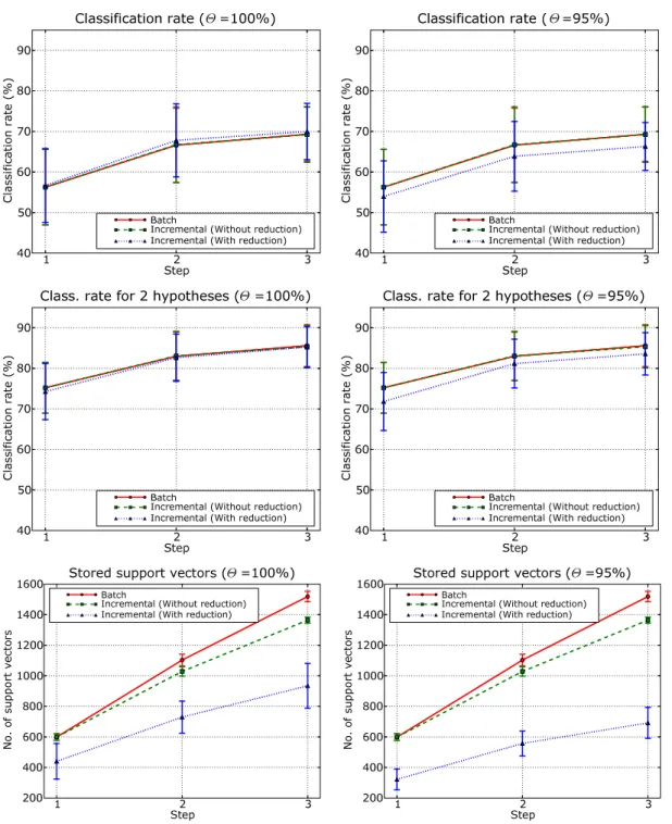
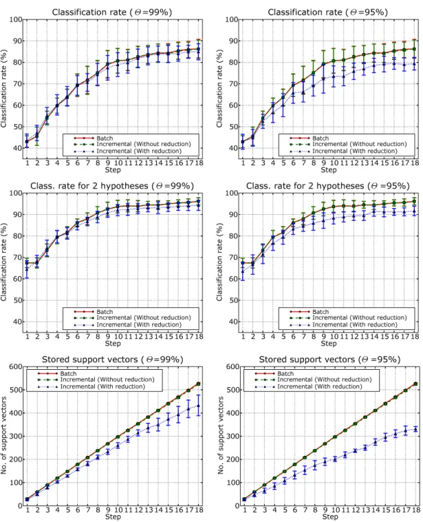
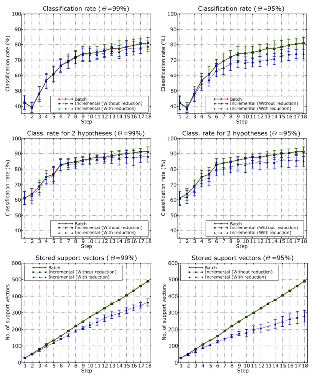
We benchmarked our new algorithm against the fixed-partition incremental SVM by repeating the experiments described in section 4.3. Fig 6 reports the results obtained on the TIPS2 database. On the left, it shows the recognition rates achieved using different values of the parameter Θ; in the middle, it shows the recognition rates obtained when considering the first two best hypothesis. Finally, on the right, the figure presents the number of support vectors stored at each incremental step. Results for the INDECS database, for both feature types, are reported in a similar fashion in Fig 7 and 8. Note that the parameter Θ decides the amount of discarded support vectors at each incremental step.
We first observe that our method controls the memory growth more successfully than the original incremental technique (Fig 6-8, top). This is especially true when it is accepted a few percent reduction in classification rate (e.g. Θ = 95% or 90%) (Fig 6-8, middle and bottom). For instance, for the TIPS2 database, the number of support vectors stored after the third step is∼32% lower than for the original incremental method. Also, for Θ = 90%, we see that the memory requirements of our algorithm after the third step are equal to those of the original method at the first iteration (Fig 6, bottom, right). Second, we observe that the gain in memory compression is always greater than the overall decrease in performance, even in the less favorable cases (see for instance results obtained on the INDECS database with Θ = 90%, Fig 7 bottom). The trade-off between performance and memory reduction becomes even better for our technique if we look at classification rates considering the best two hypothesis (Fig 6-8, middle). This would be reasonable in application like topological mapping for multi-sensory systems. A last word should be said regarding the training time at each incremental step. On one side, our method uses two algorithms in cascade while the original incremental technique uses just one. On the other side, the training time for an SVM depends on the dimension of the training set, and we have shown experimentally that our method yields far more consistent reductions. Thus, as the incremental learning proceeds, the training time of our algorithm actually becomes comparable, and eventually lower, than the original methods.
1 2 3 St e p 4 0 5 0 6 0 7 0 8 0 9 0 C la s s i f ic a t io nr a te ( % ) C la s s ific a t io n r a t e ( = 1 0 0 % ) Θ Batch Inc re m e nta l(W itho ut red uctio n) Inc re m e nta l(W ith red uctio n) 1 2 3 S te p 4 0 5 0 6 0 7 0 8 0 9 0 C la s s i f ic a t io nr a te ( % ) C la s s ific a t io n ra t e ( = 9 5 % ) Θ Ba tc h Incre m e nta l (W itho ut red uctio n) Incre m e nta l (W ith red uctio n) 1 2 3 St e p 4 0 5 0 6 0 7 0 8 0 9 0 C la s s i f ic a t io nr a te ( % ) C la s s . r a t e fo r 2 h y p o t h e s e s ( = 1 0 0 % ) Θ Batch Inc re m e nta l(W itho ut red uctio n) Inc re m e nta l(W ith red uctio n) 1 2 3 S te p 4 0 5 0 6 0 7 0 8 0 9 0 C la s s i f ic a t io nr a te ( % ) C la s s . ra t e fo r 2 h y p o t h e s e s ( = 9 5 % ) Θ Ba tc h Incre m e nta l (W itho ut red uctio n) Incre m e nta l (W ith red uctio n) 1 2 3 Ste p 2 0 0 4 0 0 6 0 0 8 0 0 1 0 0 0 1 2 0 0 14 0 0 1 6 0 0 No. o fs u p po r tv e c to r s S t o re d s u p p o rt v e ct o rs ( = 1 0 0 % ) Θ Batch Inc re m e nta l (W itho ut red uctio n) Inc re m e nta l (W ith red uctio n) 1 2 3 Ste p 2 0 0 4 0 0 6 0 0 8 0 0 1 0 0 0 1 2 0 0 14 0 0 1 6 0 0 No. o fs u p po r tv e c to r s S t o re d s u p p o rt v e ct o rs ( = 9 5 % ) Θ Batch Incre m e nta l(W itho ut red uctio n) Incre m e nta l(W ith red uctio n)
Figure 6: Results on the TIPS2 database obtained using batch SVM, the fixed-partition incremental method, and the memory controlled incremental algorithm, for two values of the parameter Θ. The top row reports classification rates obtained considering the first best hypothesis only. The middle row reports classification rates obtained considering the first two best hypotheses. The bottom row shows the number of support vectors stored at each incremental step.
1 2 3 4 5 6 7 8 9 1 0 1 1 1 2 1 3 14 1 5 1 6 1 7 1 8 S te p 4 0 5 0 6 0 7 0 8 0 9 0 1 0 0 C la s s i f ic a t io n ra te ( % ) C la s s ific a t io n ra t e ( = 9 9 % ) Θ Batc h Inc re m e nta l(W itho ut red uctio n) Inc re m e nta l(W ith red uctio n) 1 2 3 4 5 6 7 8 9 1 0 1 1 1 2 1 3 14 1 5 1 6 1 7 1 8 Ste p 4 0 5 0 6 0 7 0 8 0 9 0 1 0 0 C la s s i f ic a t io n ra te ( % ) C la s s ific a t io n ra t e ( = 9 5 % ) Θ Batch Inc re m e nta l (W itho ut red uctio n) Inc re m e nta l (W ith red uctio n) 1 2 3 4 5 6 7 8 9 1 0 1 1 1 2 1 3 14 1 5 1 6 1 7 1 8 S te p 4 0 5 0 6 0 7 0 8 0 9 0 1 0 0 C la s s i fic a t io n ra te ( % ) C la s s . ra t e fo r 2 h y p o t h e s e s ( = 9 9 % ) Θ Batc h Inc re m e nta l(W itho ut red uctio n) Inc re m e nta l(W ith red uctio n) 1 2 3 4 5 6 7 8 9 1 0 1 1 1 2 1 3 14 1 5 1 6 1 7 1 8 Ste p 4 0 5 0 6 0 7 0 8 0 9 0 1 0 0 C la s s i fic a t io n ra te ( % ) C la s s . ra t e fo r 2 h y p o t h e s e s ( = 9 5 % ) Θ Batch Inc re m e nta l (W itho ut red uctio n) Inc re m e nta l (W ith red uctio n) 1 2 3 4 5 6 7 8 9 1 0 1 1 1 2 1 3 14 1 5 1 6 1 7 1 8 Ste p 0 1 0 0 2 0 0 3 0 0 4 0 0 5 0 0 6 0 0 No. o fs u p po r tv e c to r s S t o re d s u p p o rt v e ct o rs ( = 9 9 % ) Θ Batc h Inc re m e nta l (W itho ut red uctio n) Inc re m e nta l (W ith red uctio n) 1 2 3 4 5 6 7 8 9 1 0 1 1 1 2 1 3 14 1 5 1 6 1 7 1 8 S te p 0 1 0 0 2 0 0 3 0 0 4 0 0 5 0 0 6 0 0 No. o fs u p po r tv e c to r s S t o re d s u p p o rt v e ct o rs ( = 9 5 % ) Θ Batch Inc re m e nta l (W itho ut red uctio n) Inc re m e nta l (W ith red uctio n)
Figure 7: Results on the INDECS database obtained for global features (CRFH) and Gaussian kernel using batch SVM, the fixed-partition incremental method, and the memory controlled incremental algorithm, for two values of the parameter Θ. The top row reports classification rates obtained con-sidering the first best hypothesis only. The middle row reports classification rates obtained concon-sidering the first two best hypotheses. The bottom row shows the number of support vectors stored at each incremental step.
1 2 3 4 5 6 7 8 9 1 0 1 1 1 2 1 3 14 1 5 1 6 1 7 1 8 S te p 4 0 5 0 6 0 7 0 8 0 9 0 1 0 0 C la s s i f ic a t io n ra te ( % ) C la s s ific a t io n ra t e ( = 9 9 % ) Θ Batc h Inc re m e nta l(W itho ut red uctio n) Inc re m e nta l(W ith red uctio n) 1 2 3 4 5 6 7 8 9 1 0 1 1 1 2 1 3 14 1 5 1 6 1 7 1 8 Ste p 4 0 5 0 6 0 7 0 8 0 9 0 1 0 0 C la s s i f ic a t io n ra te ( % ) C la s s ific a t io n ra t e ( = 9 5 % ) Θ Batch Inc re m e nta l (W itho ut red uctio n) Inc re m e nta l (W ith red uctio n) 1 2 3 4 5 6 7 8 9 1 0 1 1 1 2 1 3 14 1 5 1 6 1 7 1 8 S te p 4 0 5 0 6 0 7 0 8 0 9 0 1 0 0 C la s s i fic a t io n ra te ( % ) C la s s . ra t e fo r 2 h y p o t h e s e s ( = 9 9 % ) Θ Batc h Inc re m e nta l(W itho ut red uctio n) Inc re m e nta l(W ith red uctio n) 1 2 3 4 5 6 7 8 9 1 0 1 1 1 2 1 3 14 1 5 1 6 1 7 1 8 Ste p 4 0 5 0 6 0 7 0 8 0 9 0 1 0 0 C la s s i fic a t io n ra te ( % ) C la s s . ra t e fo r 2 h y p o t h e s e s ( = 9 5 % ) Θ Batch Inc re m e nta l (W itho ut red uctio n) Inc re m e nta l (W ith red uctio n) 1 2 3 4 5 6 7 8 9 1 0 1 1 1 2 1 3 14 1 5 1 6 1 7 1 8 Ste p 0 1 0 0 2 0 0 3 0 0 4 0 0 5 0 0 6 0 0 No. o fs u p po r tv e c to r s S t o re d s u p p o rt v e ct o rs ( = 9 9 % ) Θ Batc h Inc re m e nta l (W itho ut red uctio n) Inc re m e nta l (W ith red uctio n) 1 2 3 4 5 6 7 8 9 1 0 1 1 1 2 1 3 14 1 5 1 6 1 7 1 8 S te p 0 1 0 0 2 0 0 3 0 0 4 0 0 5 0 0 6 0 0 No. o fs u p po r tv e c to r s S t o re d s u p p o rt v e ct o rs ( = 9 5 % ) Θ Batch Inc re m e nta l (W itho ut red uctio n) Inc re m e nta l (W ith red uctio n)
Figure 8: Results on the INDECS database obtained for local features (SIFT) and local kernel using batch SVM, the fixed-partition incremental method, and the memory controlled incremental algo-rithm, for two values of the parameter Θ. The top row reports classification rates obtained consid-ering the first best hypothesis only. The middle row reports classification rates obtained considconsid-ering the first two best hypotheses. The bottom row shows the number of support vectors stored at each incremental step.
7
Conclusions
In this paper we explored the possibility to extend SVMs to incremental learning for visual recognition. Starting from an existing incremental SVM algorithm, we proposed a new method which is capable of learning model representations incrementally while controlling the number of support vectors to be stored. This is obtained combining the fixed-partition incremental technique with a method which reduces the number of support vectors needed to build the decision function without any loss in performance. A further extension of the algorithm permits a user-set trade-off between performance and memory reduction. An extensive experimental evaluation of the method shows its potential for computer vision applications.
This work can be extended in many ways. First, here we chose the fixed partition technique for incremental SVM, but other approximate methods might be more suitable and/or perform better. Thus, we plan to develop memory-controlled version of those algorithms and to benchmark them with our method. These methods should also be compared with other incremental methods presented in the vision literature, like for instance [14]. Second, we would like to study the algorithm’s performance as the dimension of the batch set changes, with respect to different multi-class extension, and to test it on the domain of human action recognition. A final word should be said about the training time during each incremental step. Nor our algorithm, neither the fixed-partition method can be used for on-line, continuous learning. To the best of our knowledge, this holds for any incremental SVM technique presented in the literature so far. Incorporating into our algorithm recent approaches to fast SVM training like [18] could solve this problem and open the door to real-world applications to incremental SVM.
References
[1] Syed NA, Liu H, Sung KK (1999) Incremental learning with suppoert vector machines. In Proc IJCAI’99.
[2] Downs T, Gates KE, Masters A (2001) Exact simplification of support vector solutions. JMLR 2:293-297.
[3] Torralba A, Murphy K, Freeman W (2004) Sharing features: efficient boosting procedures for multiclass object detection. In Proc CVPR’04.
[4] Viola P, Jones M (2001) Rapid object detection using a boosted cascade of simple features. In Proc CVPR’01.
[5] Grauman K, Darrell T (2005) The pyramid match kernel: discriminative classification with sets of image features. In Proc ICCV’05.
[6] Opelt A, Fussenegger M, Pinz A, Auer P (2004) Weak hypotheses and boosting for generic object detection and recognition. In Proc ECCV’04.
[7] Caputo B, Hayman E, Mallikarjuna P (2005) Class-specific material categorisation. In Proc ICCV’05.
[8] Fritz M, Leibe B, Caputo B, Schiele B (2005) Integrating representative and discriminant models for object category detection. In Proc ICCV’05.
[9] Domeniconi C, Gunopulos D (2001) Incremental support vecotr machine construction. In Proc ICDM’01.
[10] Cauwenberghs G, Poggio T (2000) Incremental and decremental support vector machine learning. In Proc NIPS’00.
[11] Mitra P, Murthy CA, Pal SK (2000) Data condensation in large databases by incremental learning with support vector machines. In Proc ICPR’00.
[12] Tong S, Koller D (2001) Support vector machine active learning with applications to text classi-fication. JMLR 2:45-66.
[13] Artaˇc M, Jogan M, Leonardis A (2002) Mobile robot localization using an incremental eigenspace model. In Proc ICRA’02.
[14] Skoˇcaj D, Leonardis A (2003) Weighted and robust incremental method for subspace learning. In Proc ICCV’03.
[15] Osuna E, Girosi F (1998) Reducing the run-time complexity of support vector machines. In Proc ICPR’98.
[16] Burges C (1996) Simplified support vector decision rules. In Proc ICML’96.
[17] Burges C, Sch¨olkopf B (1997) Improving the accuracy and speed of support vector machines. Adv in NIPS 9:375-381.
[18] Tsang IW, Kwok JT, Cheung PM (2005) Core vector machines: fast SVM training on very large data sets. JMLR, 6: 363-392.
[19] Varma M, Zisserman A (2002) Classifying images of meterial: achieving viewpoint and illumina-tion independence. In Proc ECCV’02.
[20] Oliva A, Torralba A (2001) Modeling the shape of the scene: a holistic representation of the spatial envelope. IJCV 42(3):145175.
[21] Se S, Lowe D, Little J (2002) Global localization using distinctive visual features. In Proc IROS’02. [22] Linde O. Lindeberg T (2004) Object recognition using composed receptive field histograms of
higher dimensionality. In Proc ICPR’04.
[23] Lowe D (1999) Object recognition from local scale invariant features. In Proc ICCV’99.
[24] Pronobis A and Caputo B (2005) The KTH-INDECS database. Available at:
http://cogvis.nada.kth.se/INDECS/.
[25] Cristianini N, Taylor JS (2000) An Introduction to Support Vector Machines and Other Kernel-based Learning Methods. Cambridge University Press.
[26] Vapnik V (1998) Statistical Learning Theory. Wiley and Son, New York.
[27] Wallraven C, Caputo B, Graf A (2003) Recognition with local features: the kernel recipe. In Proc ICCV’03.
[28] Peng B, Xiaugyn J, Sun Z, Wenyin L (2002) Study of SVM-based incremental learning for user adaptation in multi-class classification environment. In Proc ICONIP’02.
[29] Chang CC, Lin CJ (2001) LIBSVM : a library for support vector machines. Software available at
http://www.csie.ntu.edu.tw/~cjlin/libsvm.
[30] Golub GH, Van Loan CF (1996) Matrix Computations 3rd Edition. Johns Hopkins University Press.