Second order statistics of robust estimators of scatter.
Application to GLRT detection for elliptical signals
Romain Couillet, Abla Kammoun, Fr´
ed´
eric Pascal
To cite this version:
Romain Couillet, Abla Kammoun, Fr´
ed´
eric Pascal. Second order statistics of robust
estima-tors of scatter. Application to GLRT detection for elliptical signals. Journal of Multivariate
Analysis, Elsevier, 2016,
<
10.1016/j.jmva.2015.08.021
>
.
<
hal-01262635
>
HAL Id: hal-01262635
https://hal.archives-ouvertes.fr/hal-01262635
Submitted on 26 Jan 2016
HAL
is a multi-disciplinary open access
archive for the deposit and dissemination of
sci-entific research documents, whether they are
pub-lished or not.
The documents may come from
teaching and research institutions in France or
abroad, or from public or private research centers.
L’archive ouverte pluridisciplinaire
HAL
, est
destin´
ee au d´
epˆ
ot et `
a la diffusion de documents
scientifiques de niveau recherche, publi´
es ou non,
´
emanant des ´
etablissements d’enseignement et de
recherche fran¸
cais ou ´
etrangers, des laboratoires
publics ou priv´
es.
Second order statistics of robust estimators of scatter.
Application to GLRT detection for elliptical signals
IRomain Couilleta, Abla Kammounb, Fr´ed´eric Pascalc aTelecommunication department, Sup´elec, Gif sur Yvette, France bKing Abdullah’s University of Science and Technology, Saudi Arabia
cSONDRA Laboratory, Sup´elec, Gif sur Yvette, France
Abstract
A central limit theorem for bilinear forms of the typea∗CˆN(ρ)−1b, wherea, b∈
CN are unit norm deterministic vectors and ˆCN(ρ) a robust-shrinkage
estima-tor of scatter parametrized byρand built uponnindependent elliptical vector observations, is presented. The fluctuations ofa∗CˆN(ρ)−1b are found to be of
orderN−12 and to be the same as those ofa∗SˆN(ρ)−1bfor ˆSN(ρ) a matrix of a
theoretical tractable form. This result is exploited in a classical signal detection problem to provide an improved detector which is both robust to elliptical data observations (e.g., impulsive noise) and optimized across the shrinkage param-eterρ.
Keywords: random matrix theory, robust estimation, central limit theorem, GLRT.
1. Introduction
As an aftermath of the growing interest for large dimensional data analy-sis in machine learning, in a recent series of articles (Couillet et al., 2013a,b; Couillet and McKay, 2013; Zhang et al., 2014; El Karoui, 2013), several esti-mators from the field of robust statistics (dating back to the seventies) started to be explored under the assumption of commensurably large sample (n) and population (N) dimensions. Robust estimators were originally designed to turn classical estimators into outlier- and impulsive noise-resilient estimators, which is of considerable importance in the recent big data paradigm. Among these estimation methods, robust regression was studied in (El Karoui, 2013) which reveals that, in the largeN, nregime, the difference in norm between estimated and true regression vectors (of sizeN) tends almost surely to a positive constant
ICouillet’s work is supported by the ERC MORE EC–120133. Pascal’s work is supported
by the DGA grant XXXX.
Email addresses: romain.couillet@supelec.fr(Romain Couillet),
abla.kammoun@kaust.edu.sa(Abla Kammoun),frederic.pascal@supelec.fr(Fr´ed´eric Pascal)
which depends on the nature of the data and of the robust regressor. In parallel, and of more interest to the present work, (Couillet et al., 2013a,b; Couillet and McKay, 2013; Zhang et al., 2014) studied the limiting behavior of several classes of robust estimators ˆCN of scatter (or covariance) matricesCN based on
inde-pendent zero-mean elliptical observationsx1, . . . , xn∈CN. Precisely, (Couillet
et al., 2013a) shows that, lettingN/n <1 and ˆCN be the (almost sure) unique
solution to ˆ CN = 1 n n X i=1 u 1 Nx ∗ iCˆ −1 N xi xix∗i
under some appropriate conditions over the nonnegative functionu (correspond-ing to Maronna’s M-estimator (Maronna, 1976)), kCˆN −SˆNk
a.s.
−→ 0 in spec-tral norm as N, n → ∞ with N/n → c ∈ (0,1), where ˆSN follows a
stan-dard random matrix model (such as studied in (Silverstein and Choi, 1995; Couillet and Hachem, 2013)). In (Zhang et al., 2014), the important scenario whereu(x) = 1/x (referred to as Tyler’s M-estimator) is treated. It is in par-ticular shown for this model that for identity scatter matrices the spectrum of ˆCN converges weakly to the Mar˘cenko–Pastur law (Mar˘cenko and Pastur,
1967) in the large N, n regime. Finally, for N/n→ c ∈ (0,∞), (Couillet and McKay, 2013) studied yet another robust estimation model defined, for each
ρ∈(max{0,1−n/N},1], by ˆCN = ˆCN(ρ), unique solution to
ˆ CN(ρ) = 1 n n X i=1 xix∗i 1 Nx ∗ iCˆ −1 N (ρ)xi +ρIN. (1)
This estimator, proposed in (Pascal et al., 2013), corresponds to a hybrid robust-shrinkage estimator reminding Tyler’s M-estimator of scale (Tyler, 1987) and Ledoit–Wolf’s shrinkage estimator (Ledoit and Wolf, 2004). This estimator is particularly suited to scenarios where N/n is not small, for which other esti-mators are badly conditioned if not undefined. For this model, it is shown in (Couillet and McKay, 2013) that supρkCˆN(ρ)−SˆN(ρ)k
a.s.
−→0 where ˆSN(ρ) also
follows a classical random matrix model.
The aforementioned approximations ˆSN of the estimators ˆCN, the structure
of which is well understood (as opposed to ˆCN which is only defined implicitly),
allow for both a good apprehension of the limiting behavior of ˆCN and more
importantly for a better usage of ˆCN as an appropriate substitute for sample
covariance matrices in various estimation problems in the large N, n regime. The convergence in normkCˆN−SˆNk
a.s.
−→0 is indeed sufficient in many cases to produce new consistent estimation methods based on ˆCN by simply replacing
ˆ
CN by ˆSN in the problem defining equations. For example, the results of
(Couil-let et al., 2013b) led to the introduction of novel consistent estimators based on functionals of ˆCN (of the Maronna type) for power and direction-of-arrival
estimation in array processing in the presence of impulsive noise or rare outliers (Couillet, 2014). Similarly, in (Couillet and McKay, 2013), empirical methods were designed to estimate the parameterρwhich minimizes the expected
Frobe-nius norm tr[( ˆCN(ρ)−CN)2], of interest for various outlier-prone applications
dealing with non-small ratiosN/n.1
Nonetheless, when replacing ˆCN for ˆSN in deriving consistent estimates, if
the convergence kCˆN −SˆNk
a.s.
−→ 0 helps in producing novel consistent esti-mates, this convergence (which comes with no particular speed) is in general not sufficient to assess the performance of the estimator for large but finite
N, n. Indeed, when second order results such as central limit theorems need be established, say at rate N−12, to proceed similarly to the replacement of ˆCN
by ˆSN in the analysis, one would ideally demand thatkCˆN −SˆNk=o(N−
1 2);
but such a result, we believe, unfortunately does not hold. This constitutes a severe limitation in the exploitation of robust estimators as their performance as well as optimal fine-tuning often rely on second order performance. Concretely, for practical purposes in the array processing application of (Couillet, 2014), one may naturally ask which choice of the u function is optimal to minimize the variance of (consistent) power and angle estimates. This question remains unanswered to this point for lack of better theoretical results.
The main purpose of the article is twofold. From a technical aspect, taking the robust shrinkage estimator ˆCN(ρ) defined by (1) as an example, we first
show that, although the convergence kCˆN(ρ)−SˆN(ρ)k
a.s.
−→ 0 (from (Couillet and McKay, 2013, Theorem 1)) may not be extensible to a rateO(N1−ε), one
has the bilinear form convergence N1−εa∗( ˆCk
N(ρ)−SˆkN(ρ))b
a.s.
−→ 0 for each
ε >0, eacha, b∈CN of unit norm, and eachk∈Z. This result implies that, if
√
N a∗SˆNk(ρ)b satisfies a central limit theorem, then so does√N a∗CˆNk(ρ)bwith the same limiting variance. This result is of fundamental importance to any statistical application based on such quadratic forms. Our second contribution is to exploit this result for the specific problem of signal detection in impulsive noise environments via the generalized likelihood-ratio test, particularly suited for radar signals detection under elliptical noise (Conte et al., 1995; Pascal et al., 2013). In this context, we determine the shrinkage parameter ρwhich minimizes the probability of false detections and provide an empirical consistent estimate for this parameter, thus improving significantly over traditional sample covariance matrix-based estimators.
The remainder of the article introduces our main results in Section 2 which are proved in Section 3. Technical elements of proof are provided in the ap-pendix.
Notations: In the remainder of the article, we shall denoteλ1(X), . . . , λn(X)
the real eigenvalues ofn×nHermitian matricesX. The norm notationk·kbeing considered is the spectral norm for matrices and Euclidean norm for vectors. The symbolıis the complex √−1.
1Other metrics may also be considered as in e.g. (Yang et al., 2014) withρ chosen to
2. Main Results
LetN, n∈N,cN ,N/n, andρ∈(max{0,1−c−N1},1]. Let alsox1, . . . , xn∈
CN benindependent random vectors defined by the following assumptions.
Assumption 1 (Data vectors). For i∈ {1, . . . , n}, xi =
√
τiANwi =
√
τizi, where
• wi∈CN is Gaussian with zero mean and covarianceIN/N, independent acrossi;
• ANA∗N , CN ∈ CN×N is such that νN , N1 P N
i=1δλi(CN) → ν weakly, lim supNkCNk<∞, and N1 trCN = 1;
• τi>0 are random or deterministic scalars.
Under Assumption 1, letting τi = ˜τi/kwik for some ˜τi independent of wi, xi
belongs to the class of elliptically distributed random vectors. Note that the normalization N1 trCN = 1 is not a restricting constraint since the scalars τi
may absorb any other normalization.
It has been well-established by the robust estimation theory that, even if the τi are independent, independent of the wi, and that limn 1nP
n
i=1τi = 1
a.s., the sample covariance matrix 1
n
Pn
i=1xix∗i is in general a poor estimate
forCN. Robust estimators of scatter were designed for this purpose (Maronna,
1976; Tyler, 1987). In addition, ifN/nis non trivial, a linear shrinkage of these robust estimators against the identity matrix often helps in regularizing the estimator as established in e.g., (Pascal et al., 2013; Chen et al., 2011). The robust estimator of scatter considered in this work, which we denote ˆCN(ρ), is
defined (originally in (Pascal et al., 2013)) as the unique solution to ˆ CN(ρ) = (1−ρ) 1 n n X i=1 xix∗i 1 NxiCˆ −1 N (ρ)xi +ρIN. 2.1. Theoretical Results
The asymptotic behavior of this estimator was studied recently in (Couillet and McKay, 2013) in the regime whereN, n→ ∞in such a way thatcN →c∈
(0,∞). We first recall the important results of this article, which shall lay down the main concepts and notations of the present work. First define
ˆ SN(ρ) = 1 γN(ρ) 1−ρ 1−(1−ρ)cN 1 n n X i=1 ziz∗i +ρIN
whereγN(ρ) is the unique solution to
1 =
Z t
γN(ρ)ρ+ (1−ρ)t νN(dt).
For any κ > 0 small, define Rκ , [κ+ max{0,1−c−1},1]. Then, from
(Couillet and McKay, 2013, Theorem 1), asN, n→ ∞withcN →c∈(0,∞),
sup ρ∈Rκ ˆ CN(ρ)−SˆN(ρ) a.s. −→0.
A careful analysis of the proof of (Couillet and McKay, 2013, Theorem 1) (which is performed in Section 3) reveals that the above convergence can be refined as sup ρ∈RκN 1 2−ε ˆ CN(ρ)−SˆN(ρ) a.s. −→0 (2)
for eachε >0. This suggests that (well-behaved) functionals of ˆCN(ρ)
fluctu-ating at a slower speed thanN−12+ε for some ε >0 follow the same statistics
as the same functionals with ˆSN(ρ) in place of ˆCN(ρ). However, this result is
quite weak as most limiting theorems (starting with the classical central limit theorems for independent scalar variables) deal with fluctuations of orderN−12
and sometimes in random matrix theory of order N−1. In our opinion, the convergence speed (2) cannot be improved to a rateN−12. Nonetheless, thanks
to an averaging effect documented in Section 3, the fluctuation of special forms of functionals of ˆCN(ρ) can be proved to be much slower. Although among
these functionals we could have considered linear functionals of the eigenvalue distribution of ˆCN(ρ), our present concern (driven by more obvious
applica-tions) is rather on bilinear forms of the typea∗Cˆk
N(ρ)bfor somea, b∈C
N with
kak=kbk= 1,k∈Z.
Our first main result is the following.
Theorem 1 (Fluctuation of bilinear forms). Let a, b ∈ CN with kak =
kbk = 1. Then, as N, n → ∞ with cN → c ∈ (0,∞), for any ε > 0 and everyk∈Z, sup ρ∈Rκ N1−ε a ∗Cˆk N(ρ)b−a∗Sˆ k N(ρ)b a.s. −→0.
Some comments and remarks are in order. First, we recall that central limit theorems involving bilinear forms of the type a∗Sˆk
N(ρ)b are classical objects
in random matrix theory (see e.g. (Kammoun et al., 2009; Mestre, 2008) for
k = −1), particularly common in signal processing and wireless communica-tions. These central limit theorems in general show fluctuations at speedN−12.
This indicates, takingε < 12 in Theorem 1 and using the fact that almost sure convergence implies weak convergence, thata∗Cˆk
N(ρ)bexhibits the same
fluctu-ations asa∗Sˆk
N(ρ)b, the latter being classical and tractable while the former is
quite intricate at the onset, due to the implicit nature of ˆCN(ρ).
Of practical interest to many applications in signal processing is the case wherek=−1. In the next section, we present a classical generalized maximum likelihood signal detection in impulsive noise, for which we shall characterize the shrinkage parameterρthat meets minimum false alarm rates.
2.2. Application to Signal Detection
In this section, we consider the hypothesis testing scenario by which an N -sensor array receives a vectory∈CN according to the following hypotheses
y=
x , H0
αp+x , H1
in which α > 0 is some unknown scaling factor constant while p ∈ CN is
deterministic and known at the sensor array (which often corresponds to a steering vector arising from a specific known angle), andxis an impulsive noise distributed as x1 according to Assumption 1. For convenience, we shall take
kpk= 1.
UnderH0(the null hypothesis), a noisy observation from an impulsive source is observed while under H1 both information and noise are collected at the array. The objective is to decide onH1 versusH0 upon the observationy and prior pure-noise observationsx1, . . . , xn distributed according to Assumption 1.
Whenτ1, . . . , τnandCN are unknown, the corresponding generalized likelihood
ratio test, derived in (Conte et al., 1995), reads
TN(ρ)
H1
≷
H0
Γ for some detection threshold Γ where
TN(ρ), |y∗CˆN−1(ρ)p| q y∗Cˆ−1 N (ρ)y q p∗Cˆ−1 N (ρ)p .
More precisely, (Conte et al., 1995) derived the detectorTN(0) only valid when n ≥ N. The relaxed detector TN(ρ) allows for a better conditioning of the
estimator, in particular for n ' N. In (Pascal et al., 2013), TN(ρ) is used
explicitly in a space-time adaptive processing setting but only simulation results were provided. Alternative metrics for similar array processing problems involve the signal-to-noise ratio loss minimization rather than likelihood ratio tests; in (Abramovich and Besson, 2012; Besson and Abramovich, 2013), the authors exploit the estimators ˆCN(ρ) but restrict themselves to the less tractable finite
dimensional analysis.
Our objective is to characterize the false alarm performance of the detector. That is, provided H0 is the actual scenario (i.e. y = x), we shall evaluate
P(TN(ρ) > Γ). Since it shall appear that, under H0, TN(ρ)
a.s.
−→ 0 for every fixed Γ>0 and every ρ, by dominated convergence P(TN(ρ)>Γ) →0 which
does not say much about the actual test performance for large but finiteN, n. To avoid such empty statements, we shall then consider the non-trivial case where Γ = N−12γ for some fixed γ >0. In this case our objective is to characterize
the false alarm probability
P TN(ρ)> γ √ N .
Before providing this result, we need some further reminders from (Couillet and McKay, 2013). First define
ˆ SN(ρ),(1−ρ)1 n n X i=1 ziz∗i +ρIN.
Then, from (Couillet and McKay, 2013, Lemma 1), for each ρ∈ (max{0,1−
c−1},1], ˆ SN(ρ) ρ+γ 1 N(ρ) 1−ρ 1−(1−ρ)c = ˆSN(ρ) where ρ, ρ ρ+γ 1 N(ρ) 1−ρ 1−(1−ρ)c .
Moreover, the mapping ρ 7→ ρ is continuously increasing from (max{0,1 −
c−1},1] onto (0,1].
From classical random matrix considerations (see e.g. (Silverstein and Bai, 1995)), letting Z = [z1, . . . , zn] ∈ CN×n, the empirical spectral distribution2
of (1−ρ)1
nZ
∗Z almost surely admits a weak limitµ. The Stieltjes transform m(z),R(t−z)−1µ(dt) ofµatz∈C\Supp(µ) is the unique complex solution
with positive (resp. negative) imaginary part if =[z] >0 (resp. =[z] <0) and unique real positive solution if=[z] = 0 and<[z]<0 to
m(z) = −z+c Z (1−ρ)t 1 + (1−ρ)tm(z)ν(dt) −1 .
We denotem0(z) the derivative ofm(z) with respect toz(recall that the Stieltjes transform of a positively supported measure is analytic, hence continuously differentiable, away from the support of the measure).
With these definitions in place and with the help of Theorem 1, we are now ready to introduce the main result of this section.
Theorem 2 (Asymptotic detector performance). Under hypothesisH0, as
N, n→ ∞ withcN →c∈(0,∞), sup ρ∈Rκ P TN(ρ)> γ √ N −exp − γ 2 2σ2 N(ρ) →0
whereρ7→ρis the aforementioned mapping and σ2N(ρ), 1 2 p∗CNQ2N(ρ)p p∗Q N(ρ)p·N1 trCNQN(ρ)· 1−c(1−ρ)2m(−ρ)2 1N trCN2Q 2 N(ρ) withQN(ρ),(IN + (1−ρ)m(−ρ)CN)−1.
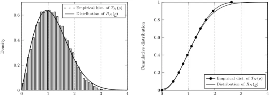
Otherwise stated,√N TN(ρ) is uniformly well approximated by a Rayleigh
dis-tributed random variableRN(ρ) with parameterσN(ρ). Simulation results are
provided in Figure 1 and Figure 2 which corroborate the results of Theorem 2 forN = 20 andN = 100, respectively (for a single value of ρthough). Com-paratively, it is observed, as one would expect, that larger values forN induce improved approximations in the tails of the approximating distribution.
0 1 2 3 4 0 0.2 0.4 0.6 Densit y Empirical hist. ofTN(ρ) Distribution ofRN(ρ) 0 1 2 3 4 0 0.2 0.4 0.6 0.8 1 Cum ul a ti v e distribution Empirical dist. ofTN(ρ) Distribution ofRN(ρ)
Figure 1: Histogram distribution function of the √N TN(ρ) versus RN(ρ), N = 20, p = N−12[1, . . . ,1]T, [C N]ij= 0.7|i−j|,cN= 1/2,ρ= 0.2. 0 1 2 3 4 0 0.2 0.4 0.6 Densit y Empirical hist. ofTN(ρ) Density ofRN(ρ) 0 1 2 3 4 0 0.2 0.4 0.6 0.8 1 Cum ul a ti v e distribution Empirical dist. ofTN(ρ) Distribution ofRN(ρ)
Figure 2: Histogram distribution function of the√N TN(ρ) versusRN(ρ), N = 100, p = N−12[1, . . . ,1]T, [C
N]ij= 0.7|i−j|,cN= 1/2,ρ= 0.2.
The result of Theorem 2 provides an analytical characterization of the per-formance of the GLRT for each ρ which suggests in particular the existence of values for ρ which minimize the false alarm probability for given γ. Note in passing that, independently ofγ, minimizing the false alarm rate is asymp-totically equivalent to minimizing σ2
N(ρ) over ρ. However, the expression of σ2
N(ρ) depends on the covariance matrixCN which is unknown to the array and
therefore does not allow for an immediate online choice of an appropriateρ. To tackle this problem, the following proposition provides a consistent estimate for
Proposition 1 (Empirical performance estimation). Forρ∈(max{0,1−
c−N1},1) andρdefined as above, let ˆσN2(ρ)be given by
ˆ σN2(ρ), 1 2 1−ρ· p∗Cˆ−N2(ρ)p p∗Cˆ−1 N (ρ)p · 1 N tr ˆCN(ρ) 1−c+cρN1 tr ˆCN−1(ρ)· 1 N tr ˆCN(ρ) 1−ρ 1 N tr ˆC −1 N (ρ)· 1 Ntr ˆCN(ρ) . Also letσˆ2
N(1),limρ↑1σˆN2(ρ). Then we have
sup ρ∈Rκ σN2(ρ)−σˆ2N(ρ) a.s. −→0.
Since both the estimation ofσN2(ρ) in Proposition 1 and the convergence in Theorem 2 are uniform overρ∈Rκ, we have the following result.
Corollary 1 (Empirical performance optimum). Let σˆ2
N(ρ)be defined as in Proposition 1 and defineρˆ∗N as any value satisfying
ˆ
ρ∗N ∈argminρ∈Rκσˆ2N(ρ)
(this set being in general a singleton). Then, for everyγ >0, P√N TN( ˆρ∗N)> γ − inf ρ∈Rκ n P√N TN(ρ)> γ o →0.
This last result states that, forN, nsufficiently large, it is increasingly close-to-optimal to use the detector TN( ˆρ∗N) in order to reach minimal false alarm
probability. A practical graphical confirmation of this fact is provided in Fig-ure 3 where, in the same scenario as in FigFig-ures 1–2, the false alarm rates for various values of γ are depicted. In this figure, the black dots correspond to the actual values taken by P(√N TN(ρ) > γ) empirically obtained out of
106 Monte Carlo simulations. The plain curves are the approximating values exp(−γ/(2σN(ρ))). Finally, the white dots with error bars correspond to the
mean and standard deviations of exp(−γ/(2ˆσN(ρ))) for each ρ, respectively.
It is first interesting to note that the estimates ˆσN(ρ) are quite accurate,
es-pecially so for N large, with standard deviations sufficiently small to provide good estimates, already for small N, of the false alarm minimizing ρ. How-ever, similar to Figures 1–2, we observe a particularly weak approximation in the (small) N = 20 setting for large values of γ, corresponding to tail events, while forN = 100, these values are better recovered. This behavior is obviously explained by the fact thatγ= 3 is not small compared to√N whenN = 20.
Nonetheless, from an error rate viewpoint, it is observed that errors of order 10−2 are rather well approximated forN = 100. In Figure 4, we consider this observation in depth by displaying P(TN(ρ) > Γ) and its approximations for N = 20 and N = 100, for various values of Γ. This figures shows that even errors of order 10−4 are well approximated for large N, while only errors of order 10−2 can be evaluated for smallN.3
0 0.2 0.4 0.6 0.8 1 10−3 10−2 10−1 100 γ= 2 γ= 3 ρ P ( √ N TN ( ρ ) > γ ) Limiting theory Empirical estimator Detector 0 0.2 0.4 0.6 0.8 1 10−2 10−1 100 γ= 2 γ= 3 ρ P ( √ N TN ( ρ ) > γ ) Limiting theory Empirical estimator Detector
Figure 3: False alarm rate P(√N TN(ρ) > γ), N = 20 (left), N = 100 (right), p = N−12[1, . . . ,1]T, [C N]ij= 0.7|i−j|,cN= 1/2. 0 0.2 0.4 0.6 0.8 1 10−4 10−3 10−2 10−1 100 N= 100 N= 20 Γ Limiting theory Detector
Figure 4: False alarm rateP(TN(ρ)>Γ) for N = 20 andN = 100,p =N−
1
2[1, . . . ,1]T,
[CN]ij= 0.7|i−j|,cN= 1/2.
3. Proof
In this section, we shall successively prove Theorem 1, Theorem 2, Propo-sition 1, and Corollary 1. Of utmost interest is the proof of Theorem 1 which
by settingρ= 0) or that would not implement a robust estimate is not provided here, being of little relevance. Indeed, a proper selection ofcN to a large value orCN with condition
number close to one would provide an arbitrarily large gain of shrinkage-based methods, while an arbitrarily heavy-tailed choice of theτidistribution would provide a huge performance gain
shall be the concern of most of the section and of Appendix Appendix A for the proof of a key lemma.
Before delving into the core of the proofs, let us introduce a few nota-tions that shall be used throughout the section. First recall from (Couillet and McKay, 2013) that we can write, for eachρ∈(max{0,1−c−N1},1],
ˆ CN(ρ) = 1−ρ 1−(1−ρ)cN 1 n n X i=1 zizi∗ 1 Nzi∗Cˆ −1 (i)(ρ)zi +ρIN where ˆC(i)(ρ) = ˆCN(ρ)−(1−ρ)1n zizi∗ 1 Nz∗iCˆ −1 N (ρ)zi. Now, we define α(ρ) = 1−ρ 1−(1−ρ)cN di(ρ) = 1 Nz ∗ iCˆ− 1 (i)(ρ)zi= 1 Nz ∗ i α(ρ) 1 n X j6=i zjzj∗ dj(ρ) +ρIN −1 zi ˜ di(ρ) = 1 Nz ∗ iSˆ −1 (i)(ρ)zi= 1 Nz ∗ i α(ρ) 1 n n X j6=i zjzj∗ γN(ρ) +ρIN −1 zi
Clearly by uniqueness of ˆCN and by the relation to ˆC(i)above,d1(ρ), . . . , dn(ρ)
are uniquely defined by theirn implicit equations. We shall also discard the parameterρfor readability whenever not needed.
3.1. Bilinear form equivalence
In this section, we prove Theorem 1. As shall become clear, the proof unfolds similarly for eachk∈Z\ {0} and we can therefore restrict ourselves to a single
value fork. As Theorem 2 relies onk=−1, for consistency, we takek=−1 from now on. Thus, our objective is to prove that, fora, b∈CN withkak=kbk= 1,
and for anyε >0, sup ρ∈Rκ N1−ε a ∗Cˆ−1 N (ρ)b−a ∗Sˆ−1 N (ρ)b a.s. −→0.
For this, forgetting for some time the indexρ, first write
a∗CˆN−1b−a∗SˆN−1b=a∗CˆN−1 α n n X i=1 1 γN − 1 di zizi∗ ! ˆ SN−1b (3) = α n n X i=1 a∗CˆN−1zi di−γN γNdi z∗iSˆ−N1b. (4)
In (Couillet and McKay, 2013), where it is shown thatkCˆN−SˆNk
a.s.
−→0 (that is the spectral norm of the inner parenthesis in (3) vanishes), the core of the
proof was to show that max1≤i≤n|di−γN|
a.s.
−→0 which, along with the conver-gence ofγN away from zero and the almost sure boundedness ofkn1P
n i=1zizi∗k
for all large N (from e.g. (Bai and Silverstein, 1998)), gives the result. A thorough inspection of the proof in (Couillet and McKay, 2013) reveals that max1≤i≤n|di−γN|
a.s.
−→0 may be improved into max1≤i≤nN
1
2−ε|di−γN|−→a.s. 0
for anyε >0 but that this speed cannot be further improved beyond N12. The
latter statement is rather intuitive sinceγN is essentially a sharp
determinis-tic approximation for N1 tr ˆCN−1 while di is a quadratic form on ˆC(−i)1; classical
random matrix results involving fluctuations of such quadratic forms, see e.g. (Kammoun et al., 2009), indeed show that these fluctuations are of orderN−12.
As a consequence, max1≤i≤nN1−ε|di−γN| and thusN1−εkCˆN−SˆNkare not
expected to vanish for smallε.
This being said, when it comes to bilinear forms, for which we shall naturally haveN12−ε|a∗Cˆ−1
N b−a
∗Sˆ−1
N b|
a.s.
−→0, seeing the difference in absolute values as then-term average (4), one may expect that the fluctuations ofdi−γN are
suf-ficiently loosely dependent acrossito further increase the speed of convergence from N12−ε to N1−ε (which is the best one could expect from a law of large
numbers aspect if thedi−γN were truly independent). It turns out that this
intuition is correct.
Nonetheless, to proceed with the proof, it shall be quite involved to work directly with (4) which involves the rather intractable terms di (as the
ran-dom solutions to an implicit equation). As in (Couillet and McKay, 2013), our approach will consist in first approximatingdi by a much more tractable
quantity. Letting γN be this approximation is however not good enough this
time sinceγN −di is a non-obvious quantity of amplitudeO(N−
1
2) which, due
to intractability, we shall not be able to average acrossiinto a O(N−1) quan-tity. Thus, we need a refined approximation ofdi which we shall take to be ˜di
defined above. Intuitively, since ˜di is also a quadratic form closely related to di, we expect di−d˜i to be of order O(N−1), which we shall indeed observe.
With this approximation in place, di can be replaced by ˜di in (4), which now
becomes a more tractable random variable (as it involves no implicit equation) that fluctuates aroundγN at the expectedO(N−1) speed.
Let us then introduce the variable ˜di in (3) to obtain
a∗CˆN−1b−a∗SˆN−1b=a∗CˆN−1 α n n X i=1 1 γN − 1 ˜ di zizi∗ ! ˆ SN−1b +a∗CˆN−1 α n n X i=1 1 ˜ di − 1 di zizi∗ ! ˆ SN−1b ,ξ1+ξ2.
We will now show that ξ1 = ξ1(ρ) and ξ2 = ξ2(ρ) vanish at the appropriate speed and uniformly so onRκ.
the explicit dependence on ˆCN. We have ξ1=a∗CˆN−1 α n n X i=1 1 γN − 1 ˜ di zizi∗ ! ˆ SN−1b =a∗SˆN−1 α n n X i=1 1 γN − 1 ˜ di ziz∗i ! ˆ S−N1b +a∗( ˆCN−1−SˆN−1) α n n X i=1 1 γN − 1 ˜ di ziz∗i ! ˆ S−N1b =a∗SˆN−1 α n n X i=1 ˜ di−γN γ2 N ziz∗i ! ˆ SN−1b −a∗SˆN−1 α n n X i=1 ( ˜di−γN)2 γ2 Nd˜i zizi∗ ! ˆ SN−1b +a∗( ˆCN−1−SˆN−1) α n n X i=1 1 γN − 1 ˜ di ziz∗i ! ˆ S−N1b ,ξ11+ξ12+ξ13.
The terms ξ12 and ξ13 exhibit products of two terms that are expected to be of order O(N−12) and which are thus easily handled. As for ξ11, it no longer
depends on ˆCN and is therefore a standard random variable which, although
involved, is technically tractable via standard random matrix methods. In order to show thatN1−εmax{|ξ
12|,|ξ13|} a.s.
−→0 uniformly in ρ, we use the following lemma.
Lemma 1. For any ε >0,
max 1≤i≤nρsup∈RκN 1 2−ε|d˜i(ρ)−γN(ρ)|−→a.s. 0 max 1≤i≤nρsup∈RκN 1 2−ε|di(ρ)−γN(ρ)|−→a.s. 0.
Note that, while the first result is a standard, easily established, random matrix result, the second result is the aforementioned refinement of the core result in the proof of (Couillet and McKay, 2013, Theorem 1).
Proof (Proof of Lemma 1). We start by proving the first identity. From (Couillet and McKay, 2013, p. 17) (taking w= −γNρα−1), we have, for each p≥2 and for each 1≤k≤n,
Eh ˜ dk(ρ)−γN(ρ) pi =O(N−p2)
where the bound does not depend onρ >max{0,1−1/c}+κ. Let now max{0,1−
1/c}+κ=ρ0< . . . < ρd√ne = 1 be a regular sampling ofRκ ind
√
We then have, from Markov inequality and the union bound on n(d√ne+ 1) events, forC >0 given,
P max 1≤k≤n,0≤i≤d√ne N 1 2−ε( ˜dk(ρi)−γN(ρi)) > C ≤KN−pε+32
for someK >0 only dependent on pandC. From the Borel Cantelli lemma, we then have maxk,i|N
1
2−ε( ˜dk(ρi)−γN(ρi))|−→a.s. 0 as long as−pε+ 3/2<−1,
which is obtained for p > 5/(2ε). Using |γN(ρ)−γN(ρ0)| ≤ K|ρ−ρ0| for
some constantK and eachρ, ρ0 ∈ R
κ (see (Couillet and McKay, 2013, top of
Section 5.1)) and similarly max1≤k≤n|d˜k(ρ)−d˜k(ρ0)| ≤K|ρ−ρ0| for all large n a.s. (obtained by explicitly writing the difference and using the fact that
kzkk2/N is asymptotically bounded almost surely), we get
max 1≤i≤nρsup∈RκN 1 2−ε|d˜i(ρ)−γN(ρ)| ≤max k,i N 1 2−ε|d˜k(ρi)−γN(ρi)|+KN−ε a.s. −→0.
The second result relies on revisiting the proof of (Couillet and McKay, 2013, Theorem 1) incorporating the convergence speed on ˜dk−γN. For convenience
and compatibility with similar derivations that appear later in the proof, we slightly modify the original proof of (Couillet and McKay, 2013, Theorem 1). We first define fi(ρ) = di(ρ)/γN(ρ) and relabel the di(ρ) in such a way that
f1(ρ)≤ . . .≤ fn(ρ) (the ordering may then depend on ρ). Then, we have by
definition ofdn(ρ) =γN(ρ)fn(ρ) γN(ρ)fn(ρ) = 1 Nz ∗ n α(ρ) 1 n X i<n zizi∗ γN(ρ)fi(ρ) +ρIN !−1 zn ≤ 1 Nz ∗ n α(ρ) 1 fn(ρ) 1 n X i<n ziz∗i γN(ρ) +ρIN !−1 zn
where we usedfn(ρ)≥fi(ρ) for eachi. The above is now equivalent to
γN(ρ)≤ 1 Nz ∗ n α(ρ) 1 n X i<n zizi∗ γN(ρ) +fn(ρ)ρIN !−1 zn.
We now make the assumption that there existsη >0 and a sequence{ρ(n)} ∈Rκ
such that fn(ρ(n)) > 1 +Nη−
1
2 infinitely often, which is equivalent to saying
dn(ρ(n))> γN(ρ(n))(1 +Nη−
1
assump-tions and the above first convergence result γN(ρ(n))≤ 1 Nz ∗ n α(ρ(n)) 1 n X i<n ziz∗i γN(ρ(n)) +ρ(n)(1 +Nη−12)IN !−1 zn = ˜dn(ρ(n))−Nη− 1 2 1 Nz ∗ n 1 n X i<n α(ρ(n))zizi∗ ρ(n)γ N(ρ(n)) + (1 +Nη−12)IN !−1 × 1 n X i<n α(ρ(n))zizi∗ γN(ρ(n)) +ρ(n)IN !−1 zn. (5)
Now, by the first result of the lemma, letting 0< ε < η, we have ˜ dn(ρ(n))−γN(ρ(n)) ≤ρmax∈Rκ ˜ dn(ρ)−γN(ρ) ≤N ε−1 2
for all large n a.s., so that, for these large n, ˜dn(ρ(n)) ≤ γN(ρ(n)) +Nε−
1 2.
Applying this inequality to the first right-end side term of (5) and using the almost sure boundedness of the rightmost right-end side term entails
0≤Nε−12 −KNη− 1 2
for someK >0 for all largena.s. But,Nε/2−1/2−KNη/2−1/2<0 for all large
N, which contradicts the inequality. Thus, our initial assumption is wrong and therefore, for each η > 0, we have for all large n a.s., dn(ρ) < γN(ρ) + Nη−1
2 uniformly onρ∈Rκ. The same calculus can be performed ford1(ρ) by
assuming thatf1(ρ0(n))<1−Nη−12 i.o. over some sequenceρ0(n); by reverting
all inequalities in the derivation above, we similarly conclude by contradiction thatd1(ρ)> γN(ρ)−Nη−
1
2 for all large n, uniformly so inRκ. Together, both
results finally lead, for eachε >0, to max 1≤k≤nρsup∈Rκ N 1 2−ε(dk(ρ)−γN(ρ)) a.s. −→0
obtained by fixingε, takingηsuch that 0< η < ε, and using maxksupρ|dk(ρ)− γN(ρ)|< Nη−
1
2 for all largena.s.
Thanks to Lemma 1, expressing ˆCN−1(ρ)−SˆN−1(ρ) as a function of di(ρ)− γN(ρ) and using the (almost sure) boundedness of the various terms involved,
we finally getN1−εξ 12 a.s. −→0 andN1−εξ 13 a.s. −→0 uniformly onρ.
It then remains to handle the more delicate termξ11, which can be further expressed as ξ11= α γ2 N a∗SˆN−1 1 n n X i=1 ( ˜di−γN)zizi∗ ! ˆ SN−1b = α γ2 N 1 n n X i=1 a∗SˆN−1ziz∗iSˆ− 1 N b ˜ di−γN .
For that, we will resort to the following lemma, whose proof is postponed to Appendix Appendix A.
Lemma 2. Let c and d be random or deterministic vectors, independent of z1,· · ·, zn, such thatmax E[kckk],E[kdkk]
≤Kfor someK >0and all integer
k. Then, for each integerp,
E 1 n n X i=1 c∗SˆN−1zizi∗Sˆ− 1 N d 1 Nz ∗ iSˆ− 1 (i)zi−γN(ρ) 2p =O N− 2p
By the Markov inequality and the union bound, similar to the proof of Lemma 1, we get from Lemma 2 (witha=c and d=b) that, for each η >0 and for each integerp≥1,
P sup
ρ∈{ρ0<...<ρd√ne}
N1−ε|ξ11|> η !
≤KN−pε+12
with K only function of η and ρ0 < . . . < ρd√ne a regular sampling of Rκ.
Takingp >3/(2ε), we finally get from the Borel Cantelli lemma that
N1−εξ11 a.s.
−→0
uniformly on {ρ0, . . . , ρd√ne} and finally, using Lipschitz arguments as in the
proof of Lemma 1, uniformly on Rκ. Putting all results together, we finally
have
sup
ρ∈RκN
1−ε|ξ1(ρ)|−→a.s. 0
which concludes the first part of the proof.
We now continue with ξ2(ρ). In order to proveN1−εξ2(ρ)−→a.s. 0 uniformly on ρ ∈ Rκ, it is sufficient (thanks to the boundedness of the various terms
involved) to prove that max 1≤i≤nρsup∈Rκ N 1−εd˜ i(ρ)−di(ρ) a.s. −→0.
To obtain this result, we first need the following fundamental proposition.
Proposition 2. For any ε >0,
max 1≤k≤nρsup∈Rκ N1−ε ˜ dk(ρ)− 1 Nz ∗ k α(ρ) 1 n X i6=k zizi∗ ˜ di(ρ) +ρIN −1 zk a.s. −→0.
Proof. By expanding the definition of ˜dk, first observe that ˜ dk− 1 Nz ∗ k α 1 n X i6=k zizi∗ ˜ di +ρIN −1 zk =α1 n X i6=k 1 Nz ∗ kSˆ −1 (k)ziz ∗ i γN−d˜i γNd˜i α 1 n X j6=k zjzj∗ ˜ dj +ρIN −1 zk.
Similar to the derivation ofξ1, we now proceed to approximating ˜diin the central
denominator and each ˜dj in the rightmost inverse matrix by the non-random γN. We obtain (from Lemma 1)
˜ dk− 1 Nz ∗ k α 1 n X i6=k zizi∗ ˜ di +ρIN −1 zk = α γ2 N 1 n X i6=k 1 Nz ∗ kSˆ −1 (k)ziz ∗ i(γN−d˜i) ˆS(−k1)zk+o(Nε−1)
almost surely, forε >0 and uniformly so onρ.
The objective is then to show that the first right-hand side term iso(Nε−1) almost surely and that this holds uniformly on k and ρ. This is achieved by applying Lemma 2 with c =d=zk. Indeed, Lemma 2 ensures that, for each
integerp,4 E 1 n X i6=k 1 Nz ∗ kS −1 (k)(ρ)ziz∗iS −1 (k)(ρ)zk 1 Nz ∗ iS −1 (i,k)(ρ)zi−γN(ρ) p =O(N− p)
From this lemma, applying Markov’s inequality, we have for eachk,
P N1−ε 1 n X i6=k 1 Nz ∗ kSˆ −1 (k)ziz ∗ iSˆ −1 (k)zk 1 Nz ∗ iSˆ −1 (i,k)zi−γN > η ≤KN−pε
for some K >0 only dependent on η > 0. Applying the union bound on the
n(n+1) events fork= 1, . . . , nand forρ∈ {ρ0, . . . , ρn}, regularn-discretization
ofRκ, we then have P max k,j N 1−ε 1 n X i6=k 1 Nz ∗ kSˆ −1 (k)zizi∗Sˆ −1 (k)zk 1 Nz ∗ iSˆ −1 (i,k)zi−γN(ρj) > η ≤KN−pε+2.
4Note that Lemma 2 can strictly be applied here forn−1 instead ofn; but since 1/n−
Takingp >3/ε, by the Borel Cantelli lemma the above convergence holds almost surely, we finally get
max k,j N1−ε ˜ dk(ρj)− 1 Nz ∗ k α(ρj) 1 n X i6=k zizi∗ ˜ di(ρj) +ρjIN −1 zk a.s. −→0.
Using theρ-Lipschitz property (which holds almost surely so for all largena.s.) on both terms in the above difference concludes the proof of the proposition.
The crux of the proof for the convergence of ξ2 starts now. In a similar manner as in the proof of Lemma 1, we define ˜fi(ρ) =di(ρ)/d˜i(ρ) and reorder
the indexes in such a way that ˜f1(ρ)≤. . .≤f˜n(ρ) (this ordering depending on ρ). Then, by definition ofdn(ρ) = ˜fi(ρ) ˜di(ρ), ˜ dn(ρ) ˜fn(ρ) = 1 Nz ∗ n α(ρ) 1 n X i<n zizi∗ ˜ di(ρ) ˜fi(ρ) +ρIn !−1 zn ≤ 1 Nz ∗ n α(ρ) 1 ˜ fn(ρ) 1 n X i<n ziz∗i ˜ di(ρ) +ρIn !−1 zn
where we used ˜fn(ρ)≥f˜i(ρ) for eachi. This inequality is equivalent to
˜ dn(ρ)≤ 1 Nz ∗ n α(ρ) 1 n X i<n ziz∗i ˜ di(ρ) + ˜fn(ρ)ρIn !−1 zn.
Assume now that, over some sequence {ρ(n)} ∈ R
κ, ˜fn(ρ(n)) >1 +Nη−1
in-finitely often for someη >0 (or equivalently,dn(ρ(n))>d˜n(ρ(n)) +Nη−1i.o.).
Then we would have ˜ dn(ρ(n))≤ 1 Nz ∗ n α(ρ (n))1 n X i<n ziz∗i ˜ di(ρ(n)) +ρ(n)(1 +Nη−1)IN !−1 zn = ˜dn(ρ(n))−Nη−1 1 Nz ∗ n 1 n X i<n α(ρ(n))z izi∗ ρ(n)d˜ i(ρ(n)) + (1 +Nη−1)IN !−1 × 1 n X i<n α(ρ(n))z iz∗i ˜ di(ρ(n)) +ρIN !−1 zn.
But, by Proposition 2, letting 0< ε < η, we have, for all largena.s., 1 Nz ∗ n α(ρ (n))1 n X i<n zizi∗ ˜ di(ρ(n)) +ρ(n)In !−1 zn≤d˜n(ρ(n)) +Nε−1
which, along with the uniform boundedness of the ˜di away from zero, leads to
˜
dn(ρ(n))≤d˜n(ρ(n)) +Nε−1−KNη−1
for some K > 0. But, as Nε−1−KNη−1 < 0 for all large N, we obtain a contradiction. Hence, for eachη >0, we have for all largena.s.,dn(ρ)<d˜n(ρ)+ Nη−1 uniformly on ρ ∈ Rκ. Proceeding similarly with d1(ρ), and exploiting
lim supnsupρmaxi|d˜i(ρ)|=O(1) a.s., we finally have, for each 0< ε < 12, that
max 1≤k≤nρsup∈Rκ N 1−ε dk(ρ)−d˜k(ρ) a.s. −→0
(for this, take anηsuch that 0< η < εand use maxksupρ|dk(ρ)−d˜k(ρ)|< Nη−1
for all largena.s.).
Getting back toξ2, we now have
N1−ε|ξ2(ρ)|=N1−ε a∗CˆN−1(ρ) α(ρ) n n X i=1 di(ρ)−d˜i(ρ) di(ρ) ˜di(ρ) zizi∗ ! ˆ SN−1(ρ)b .
But, from the above result,
N1−ε α(ρ) n n X i=1 di(ρ)−d˜i(ρ) di(ρ) ˜di(ρ) ziz∗i ≤N1−ε max 1≤k≤n dk(ρ)−d˜k(ρ) dk(ρ) ˜dk(ρ) α(ρ) n n X i=1 zizi∗ a.s. −→0
uniformly so onρ∈Rκ which, along with the boundedness ofkCˆN−1k, kSˆ −1
N k,
kak, and kbk, finally givesN1−εξ
2 a.s.
−→0 uniformly onρ∈Rκ as desired.
We have then proved that for eachε >0, sup ρ∈Rκ N 1−εa∗Cˆ−1 N (ρ)b−a ∗Sˆ−1 N (ρ)b a.s. −→0
which proves Theorem 1 fork=−1. The generalization to arbitrarykis rather immediate. Writing recursively ˆCk
N−Sˆ k N = ˆC k−1 N ( ˆCN−SˆN)+( ˆCNk−1−Sˆ k−1 N ) ˆSN, for positivekor ˆCk N−Sˆ k N = ˆC k N( ˆSN−CˆN) ˆSN−1+( ˆC k−1 N −Sˆ k−1 N ) ˆS −1 N , (3) becomes
a finite sum of terms that can be treated almost exactly as in the proof. This concludes the proof of Theorem 1.
3.2. Fluctuations of the GLRT detector
This section is devoted to the proof of Theorem 2, which shall fundamentally rely on Theorem 1. The proof will be established in two steps. First, we shall prove the convergence for eachρ∈Rκ, which we then generalize to the uniform
statement of the theorem.
Let us then fix ρ ∈ Rκ for the moment. In anticipation of the eventual
bilinear forms involved inTN(ρ) but with ˆCN(ρ) replaced by ˆSN(ρ) (note that TN(ρ) remains constant when scaling ˆCN(ρ) by any constant, so that replacing
ˆ
CN(ρ) by ˆSN(ρ) instead of by ˆSN(ρ)·
1
N tr ˆSN(ρ) as one would expect comes
with no effect).
Our first goal is to show that the vector√N(<[y∗SˆN−1(ρ)p],=[y∗Sˆ −1
N (ρ)p]) is
asymptotically well approximated by a zero mean Gaussian vector with given covariance matrix. To this end, let us denote A = [y p] ∈ CN×2 and QN = QN(ρ) = (IN+(1−ρ)m(−ρ)CN)−1. Then, from (Chapon et al., 2012, Lemma 5.3)
(adapted to our current notations and normalizations), for any HermitianB∈
C2×2and for any u∈R,
E exp ı√N utrBA∗ ˆ SN(ρ)−1−1 ρQN(ρ) A y = exp −1 2u 2∆2 N(B;y;p) +O(N−12) (6)
where we denote by E[·|y] the conditional expectation with respect to the ran-dom vectory and where
∆2N(B;y;p), cm(−ρ) 2(1−ρ)2tr ABA∗C NQ2N(ρ) 2 ρ2 1−cm(−ρ)2(1−ρ)2 1 N trC 2 NQ2N(ρ) .
Also, we have from classical central limit results on Gaussian random vari-ables Ehexpı√N utrB A∗QN(ρ)A−ΓN i = exp −1 2u 2∆02 N(B;p) +O(N−12) where ΓN , 1 ρ 1 N trCNQN(ρ) 0 0 p∗QN(ρ)p ∆0N2(B;p), B2 11 ρ2 1 N trC 2 NQ 2 N(ρ) + 2|B12|2 ρ2 p ∗C NQ2N(ρ)p.
Besides, theO(N−12) terms in the right-hand side of (6) remainsO(N−12) under
expectation overy(for this, see the proof of (Chapon et al., 2012, Lemma 5.3)). Altogether, we then have
Ehexpı√N utrBhA∗Sˆ−N1(ρ)A−ΓN ii = E exp −1 2u 2 ∆2N(B;y;p) exp −1 2u 2 ∆0N2(B;p) +O(N−12).
Note now that
A∗CNQ2N(ρ)A−ΥN
a.s.
where ΥN , 1 N trC 2 NQ 2 N(ρ) 0 0 p∗CNQ2N(ρ)p
so that, by dominated convergence, we obtain Ehexpı√N utrBhA∗Sˆ−N1(ρ)A−ΓN ii = exp −1 2u 2 ∆N2(B;p) + ∆N02(B;p) +o(1) where we defined ∆2N(B;p), cm(−ρ) 2(1−ρ)2tr (BΥ N) 2 ρ2 1−cm(−ρ)2(1−ρ)2 1 N trC 2 NQ 2 N(ρ) .
By a generalized L´evy’s continuity theorem argument (see e.g. (Hachem et al., 2008, Proposition 6)) and the Cramer-Wold device, we conclude that
√
Ny∗Sˆ−N1(ρ)y,<[y∗Sˆ−N1(ρ)p],=[y∗Sˆ−N1(ρ)p]−ZN =oP(1)
whereZN is a Gaussian random vector with mean and covariance matrix
pre-scribed by the above approximation of√NtrBA∗Sˆ−N1Afor each HermitianB.
In particular, taking B1 ∈ nh0 1 2 1 2 0 i ,h 0 2ı −ı 2 0 io
to retrieve the asymptotic vari-ances of√N<[y∗Sˆ−N1(ρ)p] and √ N=[y∗Sˆ−N1(ρ)p], respectively, gives ∆2N(B1;p) = 1 2ρ2p ∗C NQ2N(ρ)p cm(−ρ)2(1−ρ)2 1 N trC 2 NQ 2 N(ρ) 1−cm(−ρ)2(1−ρ)2 1 N trC 2 NQ 2 N(ρ) ∆0N2(B1;p) = 1 2ρ2p ∗C NQ2N(ρ)p
and thus √N(<[y∗Sˆ−N1(ρ)p],=[y∗Sˆ−N1(ρ)p]) is asymptotically equivalent to a Gaussian vector with zero mean and covariance matrix
(∆N2 (B1;p) + ∆N02(B1;p))I2= 1 2ρ2 p∗CNQ2N(ρ)p 1−cm(−ρ)2(1−ρ)2 1 N trC 2 NQ 2 N(ρ) I2.
We are now in position to apply Theorem 1. Reminding that ˆSN−1(ρ)(ρ+ 1
γN(ρ) 1−ρ
1−(1−ρ)c) = ˆS −1
N (ρ), we have by Theorem 1 fork=−1
√ N A∗ " ˆ CN−1(ρ)− ˆ SN(ρ)−1 ρ+γN(1ρ)1−1(1−−ρρ)c # A−→a.s. 0.
Since almost sure convergence implies weak convergence, √N A∗CˆN−1(ρ)A has the same asymptotic fluctuations as √N A∗Sˆ−N1(ρ)A/(N1 tr ˆSN(ρ)). Also, as
TN(ρ) remains identical when scaling ˆCN−1(ρ) by
1
N tr ˆSN(ρ), only the
fluctua-tions of√N A∗Sˆ−N1(ρ)Aare of interest, which were previously derived. We then
finally conclude by the delta method (or more directly by Slutsky’s lemma) that s N y∗Cˆ−1 N (ρ)yp∗Cˆ −1 N (ρ)p <hy∗CˆN−1(ρ)pi =hy∗CˆN−1(ρ)pi −σN(ρ)Z0=oP(1)
for someZ0 ∼N(0, I2) and
σN2(ρ), 1 2 p∗CNQ2N(ρ)p p∗Q N(ρ)p·N1 trCNQN(ρ)· 1−cm(−ρ)2(1−ρ)2 1N trCN2Q 2 N(ρ) .
It unfolds that, forγ >0,
P TN(ρ)> γ √ N −exp − γ 2 2σ2 N(ρ) →0 (7) as desired.
The second step of the proof is to generalize (7) to uniform convergence across ρ∈ Rκ. To this end, somewhat similar to above, we shall transfer the
distributionP(√N TN(ρ)> γ) to P(
√
N TN(ρ)> γ) by exploiting the uniform
convergence of Theorem 1, where we defined
TN(ρ), y ∗Sˆ N(ρ)p q y∗Sˆ N(ρ)y q p∗Sˆ N(ρ)p
and exploit aρ-Lipschitz property of √N TN(ρ) to reduce the uniform conver-gence overRκ to a uniform convergence over finitely many values ofρ.
Theρ-Lipschitz property we shall need is as follows: for eachε >0
lim δ→0Nlim→∞P sup ρ,ρ0∈Rκ |ρ−ρ0|<δ √ N|TN(ρ)−TN(ρ0)|> ε = 0. (8)
Let us prove this result. By Theorem 1, since almost sure convergence implies convergence in distribution, we have
P sup ρ∈Rκ √ N|TN(ρ)−TN(ρ)|> ε ! →0.
Applying this result to (8) induces that it is sufficient to prove (8) forTN(ρ) in place ofTN(ρ). Let η >0 small and A
η N ,{∃ρ∈Rκ, y∗Sˆ −1 N (ρ)yp∗Sˆ −1 N (ρ)p <
η}. Developing the difference TN(ρ)−TN(ρ0) and isolating the denominator according to its belonging toAηN or not, we may write
P sup ρ,ρ0∈Rκ |ρ−ρ0|<δ √ N|TN(ρ)−TN(ρ0)|> ε ≤P(AηN) +P sup ρ,ρ0∈Rκ |ρ−ρ0|<δ √ N VN(ρ, ρ0)> εη where VN(ρ, ρ0), y ∗Sˆ−1 N (ρ)p q y∗Sˆ−1 N (ρ0)y q p∗Sˆ−1 N (ρ0)p − y ∗Sˆ−1 N (ρ0)p q y∗Sˆ−1 N (ρ)y q p∗Sˆ−1 N (ρ)p.
From classical random matrix results, P(AηN) → 0 for a sufficiently small choice ofη. To prove that limδlim supnP(sup|ρ−ρ0|<δ
√
N VN(ρ, ρ0)> εη) = 0,
it is then sufficient to show that
lim δ→0lim supn P sup ρ,ρ0∈Rκ |ρ−ρ0|<δ √ N|y∗SˆN(ρ)−1p−y∗SˆN(ρ0)−1p|> ε0 = 0 (9)
for anyε0>0 and similarly fory∗SˆN(ρ)−1y−y∗SˆN(ρ0)−1y andp∗SˆN(ρ)−1p−
p∗SˆN(ρ0)−1p. Let us prove (9), the other two results following essentially the same line of arguments. For this, by (Kallenberg, 2002, Corollary 16.9) (see also (Billingsley, 1968, Theorem 12.3)), it is sufficient to prove, say
sup ρ,ρ0∈Rκ ρ6=ρ0 sup n E √ N y ∗Sˆ N(ρ)− 1p−y∗Sˆ N(ρ0)− 1p 2 |ρ−ρ0|2 <∞.
But then, remarking that
√ N y∗SˆN(ρ)−1p−y∗SˆN(ρ0)−1p = (ρ0−ρ)√N y∗SˆN(ρ)−1 IN − 1 n n X i=1 zizi∗ ! ˆ SN(ρ0)−1p
this reduces to showing that
sup ρ,ρ0∈Rκ sup n E N y∗SˆN(ρ)−1 IN − 1 n n X i=1 ziz∗i ! ˆ SN(ρ0)−1p 2 <∞.
Conditioning first onz1, . . . , zn, this further reduces to showing sup ρ,ρ0∈Rκ sup n E ˆ SN(ρ)−1 IN− 1 n n X i=1 zizi∗ ! ˆ SN(ρ0)−1p 2 <∞.
But this is yet another standard random matrix result, obtained e.g., by noticing that ˆ SN(ρ)−1 IN− 1 n n X i=1 zizi∗ ! ˆ SN(ρ0)−1p 2 ≤ 1 κ4 IN − 1 n n X i=1 zizi∗ 2
which remains of uniformly finite expectation (left norm is vector Euclidean norm, right norm is matrix spectral norm). This completes the proof of (8).
Getting back to our original problem, let us now takeε >0 arbitrary,ρ1<
. . . < ρK be a regular sampling of Rκ, and δ = 1/K. Then by (7), K being
fixed, for alln > n0(ε),
max 1≤k≤K P TN(ρi)> γ √ N −exp − γ 2 2σ2 N(ρi) < ε. (10)
Also, from (8), for small enoughδ,
max 1≤k≤KP sup ρ∈Rκ |ρ−ρk|<δ √ N|TN(ρ)−TN(ρk)|> γζ ≤P sup ρ,ρ0∈Rκ |ρ−ρ0|<δ √ N|TN(ρ)−TN(ρ0)|> γζ < ε
for all large n > n0
0(ε, ζ)> n0(ε) where ζ > 0 is also taken arbitrarily small. Thus we have, for eachρ∈Rκ and forn > n00(ε, ζ)
P TN(ρ)> γ √ N ≤P TN(ρi)> γ(1−ζ) √ N +P√N|TN(ρ)−TN(ρi)|> γζ ≤P TN(ρi)> γ(1−ζ) √ N +ε
fori≤Kthe unique index such that|ρ−ρi|< δand where the inequality holds
uniformly onρ∈Rκ. Similarly, reversing the roles ofρandρi, P TN(ρ)> γ √ N ≥P TN(ρi)> γ(1 +ζ) √ N −ε.
As a consequence, by (10), forn > n00(ε, ζ), uniformly onρ∈Rκ, P TN(ρ)> γ √ N ≤exp −γ 2(1−ζ)2 2σ2 N(ρi) + 2ε P TN(ρ)> γ √ N ≥exp −γ 2(1 +ζ)2 2σ2 N(ρi) −2ε
which, by continuity of the exponential and ofρ7→σN(ρ),5lettingζandδsmall
enough (up to growingn00(ε, ζ)), leads to
sup ρ∈Rκ P √ N TN(ρ)> γ −exp − γ 2 2σ2 N(ρ) ≤3ε
for alln > n00(ε, ζ), which completes the proof.
3.3. Around empirical estimates
This section is dedicated to the proof of Proposition 1 and Corollary 1. We start by showing that ˆσN2(1) is well defined. It is easy to observe that the ratio defining ˆσ2N(ρ) converges to an undetermined form (zero over zero) asρ↑1. Applying l’Hospital’s rule to the ratio, using the differentiation dρdSˆ−N1(ρ) =
−Sˆ−N2(ρ)(IN −n1Pizizi∗) and the limit ˆS −1 N (ρ)→IN asρ↑1, we end up with ˆ σN2(ρ)→ 1 2 p∗ n1Pn i=1zizi∗ p 1 Ntr 1 n Pn i=1zizi∗ .
Lettingε >0 arbitrary, sincep∗1nP
iziz ∗ ip−p∗CNp a.s. −→0,N1 trn1P iziz ∗ i a.s. −→1 asn→ ∞, we immediately have, by continuity of both σ2
N(ρ) and ˆσN2(ρ),
sup
ρ∈(1−κ,1]
ˆσN2(ρ)−σ2N(ρ)≤ε
for all largenalmost surely. From now on, it then suffices to prove Proposition 1 on the complementary setR0κ ,[κ+ min{0,1−c−1},1−κ]. For this, we first
recall the following results borrowed from (Couillet and McKay, 2013):
sup ρ∈Rκ ˆ CN(ρ) 1 N tr ˆCN(ρ) −SˆN(ρ) a.s. −→0.
Also, forz∈C\R+, defining ˆ SN(z),(1−ρ)1 n n X i=1 ziz∗i −zIN
5Note that it is unnecessary to ensure lim inf
NσN(ρ)>0 as the exponential would tend
(so in particular ˆS
N(−ρ) = ˆSN(ρ), for allρ∈Rκ), we have, with Ca compact
set ofC\R+ and any integerk,
sup ¯ z∈C dk dzk 1 N tr ˆS −1 N (z)− 1 N tr −z IN + (1−ρ)mN(z)CN −1 z=¯z a.s. −→0 sup ¯ z∈C dk dzk n p∗Sˆ−1 N (z)p−p ∗ −z IN + (1−ρ)mN(z)CN −1 po z=¯z a.s. −→0 where mN(z) is defined as the unique solution with positive (resp. negative)
imaginary part if=[z]>0 (resp. =[z]<0) or unique positive solution ifz <0 of mN(z) = −z+c Z (1−ρ)t 1 + (1−ρ)tmN(z) νN(dt) −1
(this follows directly from (Silverstein and Bai, 1995)).
This expression ofmN(z) can be more rewritten under the more convenient
form mN(z) =− 1−c z +c Z ν N(dt) −z−z(1−ρ)tmN(z) =−1−c z +c 1 N tr −z IN + (1−ρ)mN(z)CN −1 so that, from the above relations
sup ρ∈R0 κ mN(−ρ)− 1 −cN ρ +cN 1 N tr ˆC −1 N (ρ)· 1 N tr ˆCN(ρ) a.s. −→0 sup ρ∈R0 κ Z tν N(dt) 1 + (1−ρ)mN(−ρ)t −1−ρ 1 N tr ˆC −1 N (ρ)· 1 N tr ˆCN(ρ) (1−ρ)mN(−ρ) a.s. −→0.
Differentiating alongz the first defining identity ofmN(z), we also recall that
m0N(z) = m 2 N(z) 1−cR m(1N−(z(1)2−(1ρ−)tmρ)2t2νN(dt) N(−ρ))2 .
Now, remark that
p∗Sˆ N(ρ) −2p= d dz h p∗Sˆ N(z) −1pi z=−ρ
which (by analyticity) is uniformly well approximated by
d dz h p∗ −z IN + (1−ρ)mN(z)CN −1 pi z=−ρ = 1 ρ2p ∗Q N(ρ)p− 1 ρ(1−ρ)m 0 N(−ρ)p ∗C NQ2N(ρ)p = 1 ρ2p ∗Q N(ρ)p− 1 ρ(1−ρ) m2 N(−ρ)p∗CNQ2N(ρ)p 1−cmN(−ρ)2(1−ρ)2 1N trQ2N(ρ) .
(recall thatQN(ρ) = IN+ (1−ρ)mN(−ρ)CN −1 ). We then conclude sup ρ∈R0 κ p∗CNQ2N(ρ)p 1−cmN(−ρ)2(1−ρ)2 1N trQ2N(ρ) − p∗CˆN−1(ρ)p· 1 N tr ˆCN(ρ)−ρp ∗Cˆ−2 N (ρ)p· 1 N tr ˆCN(ρ) 2 (1−ρ)mN(−ρ)2 a.s. −→0.
Putting all results together, we obtain the expected result.
It now remains to prove Corollary 1. This is easily performed thanks to Theorem 2 and Proposition 1. From these, we indeed have the three relations
P√N TN( ˆρ∗N)> γ −exp − γ 2 2σ2 N( ˆρ ∗ N) ! a.s. −→0 P√N TN(ρ∗N)> γ −exp − γ 2 2σ2 N(ρ∗N) ! →0 exp − γ 2 2σ2 N( ˆρ ∗ N) ! −exp − γ 2 2σ∗2 N a.s. −→0
where we denoted ρ∗N any element in the argmin overρ of P(√N TN(ρ) > γ)
(andρ∗
N its associated value through the mappingρ7→ρ) andσ ∗2
N the minimum
ofσN(ρ) (i.e. the minimizer for exp(− γ
2
2σ2
N(ρ)
)). Note that the first two relations rely fundamentally on the uniform convergence supρ∈Rκ|P√N TN(ρ)> γ
− exp −γ2/(2σ2 N(ρ)) |−→a.s. 0. By definition of ρ∗N andσ∗2 N, we also have exp − γ 2 2σ∗2 N ≤min ( exp − γ 2 2σ2 N( ˆρ ∗ N) ! ,exp − γ 2 2σ2 N(ρ∗N) !) P √ N TN(ρ∗N)> γ ≤P √ N T( ˆρ∗N)> γ .
Putting things together then gives
P √ N T( ˆρ∗N)> γ −P √ N TN(ρ∗N)> γ a.s. −→0 which is the expected result.
Appendix A. Proof of Lemma 2
This section is devoted to the proof of the key Lemma 2. The proof relies on an appropriate decomposition of the quantity under study as a sum of martin-gale differences. Before delving into the core of the proofs, we introduce some
notations along with some of the key-lemmas that will be extensively used in this section.
In this section, Ej will denote the conditional expectation with respect to
theσ−fieldFjgenerated by the vectors (z`,1≤`≤j). By convention, E0= E. Useful lemmas. We shall review two key lemmas that will be extensively used, namely the generalized H¨older inequality as well as an instance of Jensen’s inequality.
Lemma 3 (Jensen Inequality, (Boyd and Vandenberghe, 2004)). LetI be a discrete set of elements of {1, . . . , n} with finite cardinality denoted by|I|. Let(θi)i∈I be a sequence of complex scalars indexed by the setI. Then, for any
p≥1, X i∈I θi p ≤ |I|p−1 n X i=1 |θi|p
Lemma 4 (Generalized H¨older inequality,(Karoui, 2008)). LetX1,· · ·, Xk bek complex random variables with finite moments of orderk. Then,
E " k Y i=1 Xi # ≤ k Y i=1 Eh|Xi| kik1 .
It remains to introduce the Burkh¨older inequalities on which the proof relies.
Lemma 5 (Burkh¨older inequality (Burkholder, 1973)). Let (Xk) n
k=1 be
a sequence of complex martingale differences sequence. For every p≥1, there existsKp dependent only onpsuch that:
E n X k=1 Xk 2p ≤Kpnpmax k E h |Xk|2p i .
LettingXk = (Ek−Ek−1)zk∗Akzk where Ak is independent of zk and noting
that Eh|Xk| 2pi ≤EhkAkk 2p Fro i
, withkAkFro ,√trAA∗, we get in particular.
Lemma 6 (Burkh¨older inequality for quadratic forms). Letz1,· · · , zn ∈
CN×1 be n independent random vectors with mean 0 and covariance CN. Let
(Aj) n
j=1 be a sequence of N×N random matrices where for all j,Aj is inde-pendent ofzj. DefineXj as Xj= (Ej−Ej−1)z∗jAjzj=z∗jEjAjzj−tr Ej−1CNAj. Then, E n X j=1 Xj 2p ≤KpkCNk 2p Fron pmax j E h kAjCNk 2p Fro i .
Preliminaries.. We start the proof by some preliminary results.
Lemma 7. Letz1,· · ·, znbe as in Assumption 1. Letc∈CN×1be independent
of z1,· · ·, zn and such that Ekckk is bounded uniformly in N for all order k. Then, for any integerp, there existsKp such that
Eh z ∗ iSˆ −1 N c pi ≤Eh z ∗ iSˆ −1 (i)c pi ≤Kp.
Proof. The first inequality can be obtained from the following decomposition:
ˆ SN−1zi= ˆ S−(i)1zi 1 + γα(ρ) N(ρ) 1 nz ∗ iSˆ −1 (i)zi
while the second follows by noticing that E|zi∗c|p≤E (c∗CNc)
p
2.
Using the same kind of calculations, we can also control the order of magnitude of some interesting quantities.
Lemma 8. The following statements hold true:
1. Denote by∆i,j the quantity:
∆i,j= 1 nz ∗ jSˆ −1 (i,j)zj− 1 ntrCN ˆ S(−i,j1). Then, for anyp≥2.
E|∆i,j| p
=O(n−p2).
2. Let iandj be two distinct integers from{1,· · ·, n}. Then,
E z ∗ iSˆ −1 (i,j)zj p =O(np2).
3. Let zi∈CN×1 be as in Assumption 1 andA be a N×N random matrix
independent ofzi and having a bounded spectral norm. Then,
E|zi∗Azi| p
=O(np).
4. Let j ∈ {1,· · ·, n} and i and k two distinct integers different from j. Then: E z ∗ iSˆ −1 (i,j)Sˆ −1 (j,k)zk p =O(np2).
Proof. Item 1) and 3) are standard results that are a by-product of (Bai and Silverstein, 2009, Lemma B.26), while Item 2) can be easily obtained from Lemma 7. As for item 4), it follows by first decomposing ˆS(−i,j1)and ˆS−(j,k1) as:
ˆ S(−i,j1)= ˆS(−i,j,k1 )−1 n α(ρ) γN(ρ) ˆ S(−i,j,k1 )zkzk∗Sˆ −1 (i,j,k) 1 +n1γα(ρ) N(ρ)z ∗ kSˆ −1 (i,j,k)zk ˆ S(−j,k1)= ˆS(−i,j,k1 )−1 n α(ρ) γN(ρ) ˆ S(−i,j,k1 )zizi∗Sˆ −1 (i,j,k) 1 + 1nγα(ρ) N(ρ)z ∗ iSˆ −1 (i,j,k)zi
The above relations serve to better control the dependencies of ˆS(−i,j1)and ˆS(−j,k1)
onzk andzi. Plugging the above decompositions onzi∗Sˆ −1 (i,j)Sˆ −1 (j,k)zk, we obtain zi∗Sˆ(−i,j1)Sˆ(−j,k1)zk=zi∗Sˆ −2 (i,j,k)zk− 1 n α(ρ) γN(ρ) zi∗Sˆ(−i,j,k1 )zkzk∗Sˆ −2 (i,j,k)zk 1 +n1γα(ρ) N(ρ)z ∗ kSˆ −1 (i,j,k)zk −1 n α(ρ) γN(ρ) zi∗Sˆ(−i,j,k2 )ziz∗iSˆ −1 (i,j,k)zk 1 +n1γα(ρ) N(ρ)z ∗ iSˆ −1 (i,j,k)zi + 1 n2 α(ρ) γN(ρ) 2 z∗ iSˆ −1 (i,j,k)zkz ∗ kSˆ −2 (i,j,k)ziz ∗ iSˆ −1 (i,j,k)zk 1 + n1γα(ρ) N(ρ)z ∗ kSˆ −1 (i,j,k)zk 1 + 1 n α(ρ) γN(ρ)z ∗ iSˆ −1 (i,j,k)zi .
The control of these four terms follows from a direct application of item 2) and 3) along with possibly the use of the generalized H¨older inequality in Lemma 4.
Core of the proof.. With these preliminaries results at hand, we are now in position to get into the core of the proof. LetβN be given by
βN = 1 n n X i=1 c∗SˆN−1ziz∗iSˆ −1 N d 1 Nz ∗ iSˆ −1 (i)zi−γN(ρ) . DecomposeβN as βN = 1 n n X i=1 c∗SˆN−1zizi∗Sˆ −1 N d 1 Nz ∗ iSˆ −1 (i)zi− 1 N trCN ˆ S(−i)1 + 1 n n X i=1 c∗SˆN−1zizi∗Sˆ− 1 N d 1 N trCN ˆ S(−i)1−γN(ρ) ,βN,1+βN,2.
The control ofβN,2follows from a direct application of Lemma 3 and Lemma 4, that is Eh|βN,2| 2pi ≤ n 2p−1 n2p n X i=1 E c ∗Sˆ−1 N zi 2p z ∗ iSˆ −1 N d 2p 1 N trCN ˆ S(−i)1−γN(ρ) 2p ≤ n 2p−1 n2p n X i=1 E c ∗Sˆ−1 N zi 6p13 E z ∗ iSˆ −1 N d 6p13 E 1 N trCN ˆ S(−i)1−γN(ρ) 6p!13
By standard results from random matrix theory (e.g. (Najim and Yao, 2013, Prop. 7.1)), we know that
E 1 NtrCN ˆ S(−i)1−γN(ρ) 6p =O(n−6p)
Hence, by Lemma 7, we finally get: E|βN,2|
2p
=O(n−2p).
While the control ofβN,2requires only the manipulation of conventional moment bounds due to the rapid convergence of N1 trCNSˆ(−i)1−γN(ρ), the analysis of βN,1is more intricate since
E 1 Nz ∗ iSˆ −1 (i)zi− 1 N trCN ˆ S−(i)1 p =O(n−p2)
a convergence rate which seems insufficient at the onset. The averaging occur-ring inβN,2shall play the role of improving this rate. To controlβN,1, one needs to resort to advanced tools based on Burkh¨older inequalities. First, decompose
βN,1as βN,1= o βN,1+E [βN,1]. As in Lemma 8, define ∆i,n1z∗iSˆ− 1 (i)zi− 1 ntrCNSˆ −1
(i). Using the relation ˆ SN−1zi= ˆ S−(i)1zi 1 + n1γα(ρ) N(ρ)z ∗ iSˆ −1 (i)zi
we get E [βN,1] = E 1 N n X i=1 c∗Sˆ(−i)1zizi∗Sˆ −1 (i)d 1 + 1 n α(ρ) γN(ρ)z ∗ iSˆ −1 (i)zi 2∆i = E 1 N n X i=1 c∗Sˆ−(i)1zizi∗Sˆ −1 (i)d 1 + n1γα(ρ) N(ρ)trCN ˆ S(−i)1 2∆i − α(ρ) γN(ρ) E 1 N n X i=1 c∗Sˆ(−i)1zizi∗Sˆ −1 (i)d∆ 2 i 2 +γα(ρ) N(ρ) 1 nz ∗ iSˆ −1 (i)zi+ 1 ntrCNSˆ −1 (i) 1 + n1γα(ρ) N(ρ)trCN ˆ S(−i)1 2 1 +γα(ρ) N(ρ) 1 nzi∗Sˆ −1 (i)zi 2 ,βN,1,1+βN,1,2
Since E [w∗Aw(w∗Bw−trB)] = E trABwhenwis standard complex Gaussian vector andA, Brandom matrices independent of w, we have
E [βN,1,1] = 1 N nE tr CNSˆ(−i)1CNSˆ(−i)1dc∗Sˆ(−i)1 1 +γα(ρ) N(ρ) 1 ntrCNSˆ −1 (i) 2 =O(n −1).
As forβN,1,2, we have for someK >0, again by Lemma 8
|βN,1,2| ≤ K n n X i=1 E c ∗Sˆ−1 (i)zi 414 E z ∗ iSˆ− 1 (i)d 414 E|∆i| 814 × E 2 + α(ρ) γN(ρ) 1 nz ∗ iSˆ −1 (i)zi+ 1 ntrCN ˆ S−(i)1 4!14 =O(1 n). We therefore have |E [βN,1]| 2p =O(n−2p).
Let’s turn to the control of
o
βN,1. For that, we decompose
o βN,1 as a sum of martingale differences as o βN,1= n X j=1 (Ej−Ej−1)βN,1 The control of E o βN,1 p
requires the convergence rate of two kinds of mar-tingale differences:
• Sum of martingale differences with a quadratic form representation of the form
n
X
j=1
For these terms, from Lemma 6, it will be sufficient to show that maxjEkAjk2Frop =
O(n−3p) in order to obtain the required convergence rate.
• Sum of martingale differences with more than one occurrence of zj and zj∗. In this case, this sum is given by:
n X j=1 (Ej−Ej−1) n X i=1,i6=j εi
whereεjare small random quantities depending onz1,· · · , zn. According
to Lemma 5, we have n X j=1 (Ej−Ej−1) n X i=1,i6=j εi 2p =O(n−2p) provided that E X i=1,i6=j εi 2p =O(n−3p).
The control of the above sum will rely on successively using Lemma 3 to get E X i=1,i6=j εi 2p ≤n2p−1 n X i=1 E|εi| 2p
and controlling maxiE|εi|
2p
.
With this explanation at hand, we will now get into the core of the proofs. We first have o βN,1= n X j=1 (Ej−Ej−1) 1 N n X i=1 c∗Sˆ−N1zizi∗d∆i = n X j=1 (Ej−Ej−1)c∗SˆN−1zjzj∗d∆j + n X j=1 (Ej−Ej−1) 1 N n X i=1,i6=j c∗SˆN−1zizi∗d∆i , n X j=1 Wj,1+ n X j=1 Wj,2.
In order to prove that E Pn j=1Wj,1 =O(n −2p), it is sufficient to show E|Wj,1|=O(n−3p)