Clustering-Initialized Adaptive
Histograms and Probabilistic Cost
Estimation for Query Optimization
zur Erlangung des akademischen Grades eines
Doktors der Ingenieurwissenschaften
von der Fakultät für Informatik
des Karlsruher Instituts für Technologie (KIT)
genehmigte
Dissertation
von
Andranik Khachatryan
aus Jerewan
Tag der mündlichen Prüfung:
30.04.2012
Erster Gutachter:
Prof. Dr.-Ing. Klemens Böhm
Acknowledgments
First of all, I would like to express my deepest gratitude to Prof. Klemens Böhm, who supervised this thesis, for the invaluable insight he brought into this work. His dedication and work ethics served as an example for me and everyone else in the group. Without his encouragement, willingness to discuss and patience I would not have made it.
I would like to thank also Prof. Bernhard Seeger, my second advisor, for his will-ingness to undertake the ungratifying task of reading and commenting on the thesis.
I am greatly obliged to Emmanuel Müller with whom we worked together for the last year and a half. He brought invaluable insight and experience into the topic. Working with him was both productive and enjoyable.
Peter J. Haas gave me a draft of his review on histograms. This review greatly influenced my view on the whole subject. The chapter on histograms in this thesis follows Peter’s conventions on histogram categorization.
My family had all the patience and showed all the support during those years that I was doing this work. I would not have gotten here without them.
Last but not least, I want to thank my friend and office-mate Björn-Oliver Hart-mann with whom we spent long hours in discussions, about our research topics and not only. We had quite different perspective on a variety of things, and our discus-sions were very interesting. He was and is always willing to help and support.
Contents
1 Zusammenfassung der Arbeit 1
1.1 Initialisierung von Histogrammen . . . 2
1.1.1 Probleme von Selbstoptimierungsansätzen . . . 2
1.1.2 Subraum-Clustering und Histogramme . . . 2
1.2 Nicht-lineare Kosten- und Kardinalitätsverteilungen . . . 4
2 Thesis Abstract 1 2.1 Histogram Initialization . . . 1
2.1.1 Problems With Self-Tuning Approaches. . . 1
2.1.2 Subspace Clustering and Histograms . . . 2
2.2 Non-linear Costs and Cardinality Distributions. . . 3
3 Introduction 5 3.1 Query Optimization . . . 5
3.1.1 Query Plan Costs . . . 6
3.2 Selectivity and Cardinality . . . 6
3.2.1 Properties of Selectivity Estimates . . . 11
3.2.2 Query types . . . 12
3.3 Requirements for Selectivity Estimation . . . 14
3.3.1 Multi-dimensional Predicates . . . 15
3.4 Summary . . . 16
4 Histograms 17 4.1 First Histograms . . . 17
4.1.1 The Equi-Width Histogram . . . 17
4.1.2 The Equi-Depth histogram . . . 19
4.1.3 Histograms On Relational Data . . . 19
4.1.4 Histogram Categorization . . . 21
4.2 Estimation Schemes . . . 22
4.2.1 Equi-Distant Schemes . . . 22
4.2.2 Other Approximation Schemes . . . 24
4.2.3 Bucketing Schemes . . . 24
4.3 Static Multi-Dimensional Histograms . . . 25
4.4 Dimensionality Reduction Techniques . . . 27
4.5 Self-Tuning Histograms . . . 28
4.5.1 The STHoles Histogram . . . 28
4.6 Consistent Selectivity Estimation . . . 38
4.6.1 ISOMER: A Consistent Self-tuning Histogram . . . 38
4.6.2 Consistent Estimates from Partial Statistics . . . 41
4.7 Assessing Histogram Precision . . . 42
4.7.1 Error Metrics . . . 43
4.7.2 Data Sets. . . 44
4.7.3 Workloads . . . 47
4.8 Other Uses of Histograms . . . 48
4.8.1 Skyline Queries . . . 48 4.8.2 Top-k Queries . . . 50 4.9 Summary . . . 51 5 Histogram Initialization 53 5.1 Introduction . . . 53 5.2 Subscpace Clustering . . . 54 5.3 Cluster Transformation . . . 55
5.3.1 The Optimal RR for Selectivity Estimation . . . 56
5.3.2 Cluster-to-Bucket Transformation . . . 59
5.4 Experiments . . . 61
5.4.1 Setup . . . 61
5.4.2 Estimation Precision . . . 62
5.4.3 Memory-efficiency w.r.t. different initializations . . . 65
5.4.4 Scalability w.r.t. data dimensionality . . . 69
5.5 Conclusions and Future Work . . . 69
6 Robust Self-Tuning Histograms 71 6.1 Introduction . . . 71
6.2 Self-Tuning Histograms and Their Problems . . . 73
6.3 Problems with Self-Tuning . . . 74
6.3.1 Sensitivity to Learning . . . 74
6.3.2 Stagnation . . . 75
6.3.3 Dimensionality . . . 81
6.4 Subspace Clustering and Histogram Initialization . . . 82
6.4.1 Initialization by Subspace Clusters . . . 82
6.4.2 Analysis on Subspace Solution . . . 83
6.5 Experiments . . . 87
6.5.1 Experimental Setup . . . 87
6.5.2 Accuracy . . . 88
Contents
7 Probabilistic Cost Estimation 95
7.1 Introduction . . . 95
7.2 Related Work . . . 99
7.3 Definitions and Notation . . . 100
7.4 Cardinality Distributions over Multi-Dimensional Histograms . . . 101
7.4.1 The Sample-Based Method . . . 101
7.4.2 The Uniformity Method . . . 103
7.5 Comparison Metrics . . . 106
7.5.1 Query-Plan Costs . . . 106
7.5.2 Comparing Cardinality-Estimation Methods . . . 107
7.5.3 Optimality Conditions . . . 108 7.6 Experimental Evaluation . . . 113 7.6.1 Experiments – Overview . . . 114 7.6.2 Experiments – Data . . . 114 7.6.3 Experiments . . . 115 8 Conclusions 119 8.1 Self-Tuning Histograms And Their Problems . . . 119
8.2 Improved Cost Model . . . 120
List of Figures
3.1 Cost graph for two plans, table scan and index seek . . . 9
3.2 The range query as a rectangle in the two-dimensional space . . . . 13
4.1 An Equi-Width histogram with 6 buckets . . . 18
4.2 An Equi-Width histogram with 3 buckets . . . 18
4.3 An Equi-Depth histogram with 3 buckets . . . 19
4.4 A sample distribution . . . 23
4.5 An Equi-Depth approximation of the distribution using a single bucket. 23 4.6 An Equi-distant approximation of the distribution, using 1 bucket with 2 non-zero values. . . 23
4.7 Creation of a multi-dimensional Equi-Depth histogram . . . 26
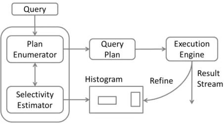
4.8 The query execution cycle and a self-tuning histogram . . . 28
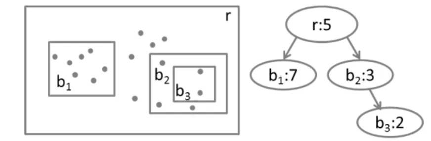
4.9 An STHoles histogram on the left and the bucket tree on the right . . 29
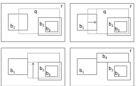
4.10 An STHoles histogram with queryq . . . 30
4.11 Two possible ways of shrinkingq∩binto rectangular shape . . . . 31
4.12 Progressive shrinking ofq∩b . . . 32
4.13 Sibling-sibling merge ofb1 andb2 . . . 33
4.14 Sibling-sibling merge ofb1 andb2 . . . 34
4.15 Sibling-sibling merge ofb1 andb2 . . . 36
4.16 Available query feedback for theCarsrelation. . . 39
4.17 Available query feedback for theCarsrelation. . . 40
4.18 A new query intersecting with an existing bucket. . . 40
4.19 New bucket added according to the STHoles drilling procedure. . . 40
4.20 New bucket added according to the ISOMER drilling procedure. . . 41
4.21 TheCrossdataset . . . 44
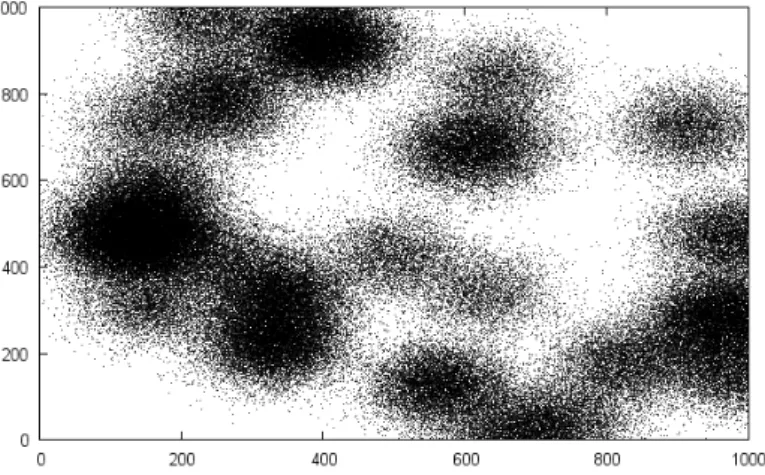
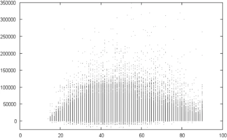
4.22 TheGaussdataset with 500,000 tuples . . . 46
4.23 TheGaussdataset with 200,000 tuples . . . 46
4.24 TheCensusdataset . . . 47
4.25 A hotel skyline . . . 48
4.26 A hypothetical point and its dominated region (in grey) . . . 49
4.27 The histogram on the left and the approximate skyline of the hypo-thetical points on the right. . . 49
5.1 A cluster and a candidate RR . . . 56
5.3 Error vs bucket count for 2-dimensional space, 10,000 queries . . . 63
5.4 Error vs bucket count for 2-dimensional space, 50,000 queries . . . 63
5.5 Error vs bucket count for 3-dimensional space, 10,000 queries . . . 64
5.6 Error vs bucket count for 3-dimensional space, 50,000 queries . . . 64
5.7 Error vs bucket count for 4-dimensional space, 10,000 queries . . . 65
5.8 Error vs bucket count for 4-dimensional space, 50,000 queries . . . 65
5.9 Error vs bucket count for 5-dimensional space, 10,000 queries . . . 66
5.10 Error vs bucket count for 5-dimensional space, 50,000 queries . . . 66
5.11 Error vs bucket count for 10-dimensional space, 10,000 queries . . . 67
5.12 Error vs bucket count for 10-dimensional space, 50,000 queries . . . 67
5.13 Execution time against the dimensionality . . . 69
6.1 The queries and resulting histograms for two queries. . . 74
6.2 The data space and the clusterC . . . 78
6.3 The cluster. . . 79
6.4 The cluster with one row detected (left) and the second row detected (right). . . 79
6.5 A bucket which is a result of several merges which occurred horizon-tally on the second row of the cluster. . . 80
6.6 A histogram with two clusters, each of the clusters has a dense core. 81 6.7 On the left, the cluster found. On the right, the dashed rectangle is the MBR of the cluster. The solid rectangle on the right is the extended BR. . . 83
6.8 The histogramH0, with clusterC as a bucket. The dashed rectangle is the incoming queryq. . . 84
6.9 ClusterCwith several dense subregions . . . 86
6.10 Error comparison forCross[1%]setting . . . 88
6.11 Error comparison forGauss[1%]setting . . . 89
6.12 Error comparison forSky[1%]setting. The meaning of the green line ”Initialized (Reversed)” is explained in Section 6.5.3. . . 90
6.13 Error comparison forSky[2%]setting . . . 91
6.14 Error comparison of heavily-trained vs Initialized histograms,Sky− 1%setting. . . 92
7.1 Hash join plans for the example query. . . 96
7.2 The dependency of the join cost fromσ(O) . . . 96
7.3 The estimated (left) and real plan costs for the TPC-H query 9 . . . 97
7.4 A histogram with queryq . . . 102
7.5 Queryq, partially intersecting with bucketb. . . 104
7.6 -measures for theGauss[U nif orm,1%]setting . . . 115
7.7 -measures for theArray[U nif orm,1%]setting . . . 116
List of Figures
List of Tables
3.1 A sample relation Cars . . . 8
4.1 Orders table with order-id and amount of order . . . 20
5.1 Parameters values of experiments . . . 62 5.2 Memory requirements for Mineclus compared to STHoles, to achieve
same or better error rates as STHoles. Data set contains 10,000 tuples. 68 5.3 Memory requirements for Mineclus compared to STHoles, to achieve
same or better error rates as STHoles. Data set contains 50,000 tuples. 68
6.1 Dimensionalities and tuple counts of our datasets . . . 87 6.2 Clusters found in theSkydataset and the dimensions they do not use 91 7.1 Description of data sets . . . 115
1 Zusammenfassung der Arbeit
Datenbanken ermöglichen es ihren Nutzern, deklarative Anfragen zu stellen. Der Nutzer beschreibt die Daten, die er von der Datenbank erhalten möchte, und ist davon befreit zu spezifizieren, wie die Daten gewonnen werden sollen.
Es existieren viele Alternativen eine Anfrage abzuarbeiten. Diese Alternativen werden auch als Ausführungspläne bezeichnet. Eine Komponente des Datenbank-Management Systems, der sogenannte Anfrageoptimierer, entscheidet, wie ein ef-fizienter Ausführungsplan gewählt wird. Bisher nutzen Optimierer kostenbasierte Optimierungen. Näherungen für die Ausführungskosten werden für viele Ausfüh-rungspläne berechnet und ein Ausführungsplan mit geringen Kosten wird ausgewählt. Die Ausführungskosten sind eine gewichtete Funktion der Systemressourcen, die ge-braucht werden, um die Anfrage auszuführen. Beispiele solcher Systemressourcen sind CPU-Zeit oder die Anzahl von Ein- und Ausgabeoperationen.
Um eine angebrachte Kostenschätzung zu erreichen, benötigt der Optimierer eine Schätzung der Größe von Teilanfragen. Dies ist zum Beispiel dann wichtig, wenn die Verbund-Reihenfolge (engl. join order) von Relationen bestimmt wird. Um die Größe von Teilanfragen zu schätzen, muss der Optimierer die Selektivität von Anfrage-Prädikaten kennen.
Die wesentliche Datenstruktur zur Bestimmung von Selektivitäten in Datenbanken sind Histogramme. Selbstoptimierende Histogramme sind eine Klasse von Histo-grammen, die die Ergebnisse von bereits existierenden Anfragen nutzen, um sich selbst anzupassen. Dies ist eine Art des überwachten Lernens. Selbstoptimierende Histogramme sind in der Lage, Initialisierungskosten zu amortisieren, sich an die Anfragelast anzupassen und sind nach allgemeinem Verständnis eine flexible Alter-native zu statischen Ansätzen, welche Histogramme anlegen und sie dann unverän-dert bestehen lassen. Histogramme haben eine Vielzahl von Anwendungen in Daten-banken und verwandten Anwendungen. Wir haben die Anfrageoptimierung erwähnt, weitere Beispiele sind die Top-k Anfrageverarbeitung, die näherungsweise Beant-wortung von Anfragen, Skyline Anfragen, sowie geographische und spatio-temporale Datenbanken.
Diese Arbeit hat zwei Hauptbeträge. Der erste Beitrag sind signifikante Verbesse-rungen von selbstoptimierenden Histogrammen durch Initialisierung (Abschnitt 1.1). Der zweite Beitrag ist die Verallgemeinerung von selbstoptimierenden Histogram-men zur Unterstützung von nicht-linearen Kostenmodellen (Abschnitt 1.2).
1.1 Initialisierung von Histogrammen
1.1.1 Probleme von Selbstoptimierungsansätzen
Obwohl sie viele attraktive Eigenschaften besitzen, haben Selbstoptimierungsansätze mehrere Nachteile. Die Hauptannahme hinter selbstoptimierenden Histogrammen ist, dass – gegeben, dass genug Anfragenergebnisse zum Lernen vorhanden sind – sie in der Lage sind, die zugrunde liegenden Daten akkurat zu erfassen. Wir zeigen, dass dies nicht der Fall ist. Die als erstes gelernten Anfragen haben für selbstoptimierende Histogramme eine größere Bedeutung als Anfragen, die später gelernt werden. (Dies ist ein übliches Verhalten auch bei anderen überwachten Lernverfahren.) Die ersten Anfragen definieren die obersten Ebenen der Histogramm-Strukturen. Wenn diese Strukturen schlecht sind, dann ist subsequentes Lernen normalerweise nicht in der Lage, dies zu beheben. Daher kann die Reihenfolge der gelernten Anfragen einen großen Einfluss auf die Strukturen und die Genauigkeit der Schätzungen von His-togrammen haben. Wir nennen dies: Sensibilität bezüglich Lernen. Ein assoziiertes Problem ist, dass selbstoptimierende Methoden Schwierigkeiten haben, komplexe Datenstrukturen in hochdimensionalen Räumen zu erfassen. Dies liegt in der Tat-sache begründet, dass es schwierig ist, dichte Daten-Regionen in Projektionen von hochdimensionalen Räumen, insbesondere wenn wir die Daten nicht selbst erfassen können, zu finden, während lediglich Anfrageergebnisse begutachtet werden können. Wir wollen diese Probleme lösen, ohne die Vorteile von selbstoptimierenden Meth-oden, namentlich ihre Fähigkeit, sich an die Arbeitslast anzupassen, und die Fähigkeit, Initialisierungskosten zu amortisieren, zu verlieren. Wir stellen das Konzept der Histogramm-Initialisierung vor. Die Idee ist, mit wenigen, aber vorsichtig gewählten, Regionen [engl. buckets] zu starten. Wir stellen im Folgenden dar, wie dies funktion-iert.
1.1.2 Subraum-Clustering und Histogramme
Wir zeigen formal und experimentell, dass die Initialisierung von selbstoptimieren-den Histogrammen die Genauigkeit von Schätzungen erhöht. Die hier beschriebe-nen Ergebnisse basieren auf [KMBK11]. Zur Initialisierung nutzen wir Subraum-Clustering-Algorithmen, die kompakte, dichte Cluster von Objekten in Projektionen von hochdimensionalen Räumen finden.
Initiale Regionen definieren wenige, aber vorsichtig gewählte Top-Level Regio-nen für Histogramme. Diese RegioRegio-nen verhindern, dass schlecht zu lerRegio-nende An-fragen die gesamte Datenstruktur ruinieren. Sie machen Histogramme weniger ab-hängig von der Qualität und der Reihenfolge der ersten gelernten Anfragen. Das Histogramm ist dann in der Lage, zu besseren Regions-Konfigurationen zu kon-vergieren, und bleibt nicht in lokalen Optima hängen. Dies berücksichtigt die Sensi-bilität bezüglich Lernen.
1.1. INITIALISIERUNG VON HISTOGRAMMEN
Jeder Subraum-Cluster ist mit einer Menge von relevanten Dimensionen verbun-den. Genauer: Wenn einige Dimensionen irrelevant für einen bestimmten Cluster sind, dann werden sie verworfen. Dies erlaubt es, dass Histogramme schwer zu ent-deckende Korrelationen speichern, und dass sie gleichzeitig speichereffizient sind.
Wir zeigen, dass der Berechnungsoverhead für die Initialisierung gering ist und dass er, gemessen an der Verbesserung der Schätzgenauigkeit, leicht zu akzeptieren ist.
Als nächstes vergleichen wir verschiedene Subraum-Clustering-Algorithmen in Bezug auf ihre Leistungsfähigkeit als Initialisierer. Einige Subraum-Clustering-Al-gorithmen können Cluster von beliebiger Form ausgeben, so dass wir sie in eine histogrammfreundliche Darstellung transformieren müssen.
Formale Ergebnisse. Wir definieren Sensibilität bezüglich Lernen formal. Wir zeigen, dass selbst für die einfachsten Datensätze eine angemessene Initialisierung die Sensibilität des Lernens reduziert. Das bedeutet, dass Initialisierung den nega-tiven Effekt von "schlechtem" Lernen begrenzt.
Wir formalisieren den Begriff der Transformation von Clustering-Ergebnissen zu Histogramm-Regionen. Danach definieren wir Klassen von Transformationen, die nützliche Eigenschaften haben. Als nächstes zeigen wir, dass es zu teuer ist, strikt optimale Clustering-zu-Histogramm-Transformationen zu finden. Stattdessen schla-gen wir eine Heuristik vor, die gute Transformationen findet.
Experimentelle Ergebnisse. Wir haben Experimente durchgeführt, deren Auf-bau dem von in verwandten Arbeiten vorgenommenen Experimenten entspricht.
Wir haben sechs Subraum-Clustering-Algorithmen als Initialisierer verglichen. Ei-ner von ihnen zeigte konsistente Verbesserungen (bei allen Experimenten) gegenüber uninitialisierten Histogrammen sowie gegenüber anderen Clustering-Initialisierungs-verfahren. Um die gleichen Fehlerraten wie die uninitialisierten Verfahren zu erre-ichen, benötigt dieser Algorithmus achtmal so wenig Speicher für die Histogramme. Wir zeigen, dass selbstoptimierende Histogramme sensibel bezüglich Lernen sind. Ohne Initialisierung ist das Histogramm nicht in der Lage, selbst simple Datenstruk-turen zu lernen. Für komplexe Datensätze garantiert die Initialisierung, dass der Fehler des Histogramms um 50% reduziert wird. Als nächstes zeigen wir, dass die Effekte der Initialisierung nachhaltig sind. Selbst nach intensivem Lernen kann ein uninitialisiertes Histogramm nicht an die Leistung der initialisierten Version anknüp-fen.
Insgesamt erlaubt es die Initialisierung von selbstoptimierenden Histogrammen, die Sensibilität bezüglich Lernen zu verlieren, und es verbessert die Genauigkeit der Schätzung signifikant. Gleichzeitig werden die positiven Eigenschaften von selbstop-timierenden Methoden bewahrt.
1.2 Nicht-lineare Kosten- und
Kardinalitätsverteilungen
Relationale Kostenoptimierer nehmen an, dass die Kosten eine lineare Funktion der Selektivität sind. Aktuelle Forschungsergebnisse zeigen, dass diese Annahme zu un-genauen Kostenschätzungen führen kann. Genauer: Gewisse Anwendungen wie die Top-k Anfrageverarbeitung muss mit Kostenmodellen umgehen können, die nicht einmal nährungsweise linear sind.
Ein lineares Kostenmodell in ein nicht-lineares zu überführen, hat zur Konsequenz, dass auch das Selektivitätsabschätzungssubsystem angepasst werden muss. Statt einer einzelnen Selektivitätsschätzung benötigt der Optimierer nun eine Wahrschein-lichkeitsverteilung über mögliche Selektivitäten. Diese Verteilungen müssen präzise sein, müssen fundiert theoretisch abgeleitet sein und sollten wenig Overhead erzeu-gen. Die Unterstützung verteilungsbasierter Schätzungen ist eine große Heraus-forderung, beim Wechsel hin zu einem nicht-linearen Kostenmodell. Verteilungs-basierte Selektivitätsschätzungen in mehrdimensionalen Räumen sind der zweite Bei-trag dieser Arbeit. (Die hier beschriebenen Ergebnisse basieren auf [KB10]).
Wir zeigen, wie der Übergang von einem Modell basierend auf einer einzigen Schätzung nahtlos durch die Nutzung von ausschließlich im Histogramm existieren-den Informationen bewältigt werexistieren-den kann. Die Wahrscheinlichkeitsverteilung wird durch die Annahme abgeleitet, dass ein Tupel mit gleicher Wahrscheinlichkeit an jedem Punkt der Region vorkommen kann.
Unsere Experimente zeigen, dass wahrscheinlichkeitsbasierte Kostenschätzungen genauer sind als konventionelle. Die Wahrscheinlichkeitsverteilungen haben darüber hinaus einige interessante theoretische Eigenschaften.
Formale Ergebnisse. Für jedes Histogramm existieren viele Datensätze, die zu diesem kompatibel sind. Wir zeigen das Folgende: Sind alle kompatiblen Daten-sätze gleichwahrscheinlich, so sind unsere verteilungsbasierten Schätzungen optimal. Die Annahme, dass alle kompatiblen Datensätze gleichwahrscheinlich sind, ist eine natürliche Annahme, wenn wir keine weiteren Informationen über die Verteilung der möglichen Datensätze besitzen.
Experimentelle Ergebnisse. Experimente zeigen, dass für nicht-lineare Kosten-funktionen aus der Literatur verteilungsbasierte Schätzungen (in allen Experimenten) besser als konventionelle Schätzungen sind. In einigen Versuchen ist der Fehler der verteilungsbasierten Schätzungen nur halb so groß wie bei den Vergleichsverfahren. Nicht-lineare Kostenmodelle sind essentiell für präzise Kostenschätzungen in Daten-banken und vergleichbaren Anwendungen. Wir zeigen, dass nicht-lineare Kosten-modelle durch existierende Datenstrukturen für Selektivitätsschätzungen unterstützt werden können, ohne dass zusätzlicher Overhead entsteht.
2 Thesis Abstract
Databases enable users to issue declarative queries. The user describes the data
he wants to obtain from the database, and is relieved from specifying how the data should be retrieved.
There are numerous alternative ways to execute a query. These are so called ex-ecution plans. A component in the database management system called theQuery Optimizerdecides how to pick an efficient execution plan. To this end, the optimizer deploys cost-based optimization. Approximate execution costs are calculated for var-ious plans, and one with low cost is chosen. The execution cost is a weighted function of the system resources needed to execute the query. Examples of such system re-sources are the CPU time or the number of I/O operations.
In order to come up with reasonable cost estimates, the optimizer needs to estimate the size of sub-queries. This is important, for instance, when choosing the join order of the relations. To estimate the sizes of sub-queries, the optimizer needs to know the selectivityof the query predicates.
The main data structures used for selectivity estimation in databases are histo-grams. Self-tuning histograms are a class of histograms which use the results of already executed queries to refine themselves. This is a sort of supervised learning. Self-tuning histograms are able to amortize the construction costs, adapt to the query workload and are generally considered to be a flexible alternative to static approaches which construct the histogram and leave it unchanged.
Histograms in general have multiple uses in databases and related applications. We mentioned Query Optimization, other examples are Top-k query processing, approx-imate query answering, Skyline queries, geographical and spatio-temporal databases. There are two main contributions in this thesis. The first contribution is about significant improvement of self-tuning histograms by Initialization (Section 2.1).
The second contribution is about generalization of self-tuning histograms to sup-port non-linear cost models (Section 2.2).
2.1 Histogram Initialization
2.1.1 Problems With Self-Tuning Approaches.
Despite their attractive features, self-tuning approaches have several disadvantages. The main assumption behind self-tuning histograms is that, given enough query
re-sults to learn, they will be able to accurately capture the underlying data distribution. We show that this is not the case. For self-tuning histograms, the first learning queries have a great importance compared to the queries that come later in the workload. (This is commonplace with other supervised learning algorithms as well). These first queries define the top-level structure of the histogram. If this structure is bad, the sub-sequent learning is usually unable to fix it. Thus, the order of the learning queries can have a big influence on the structure and the estimation precision of the histogram. We call thissensitivity to learning.
An associated problem is that self-tuning methods struggle to capture complex data correlations in high-dimensional spaces. This stems from the fact that it is hard to find dense data regions in projections of high-dimensional space, particularly if we do not access the data itself, but only look at query-execution results.
We want to solve these problems without sacrificing the advantages of the self-tuning methods, namely their ability to adapt to the workload and to amortize the construction costs.
We introduce the concept ofHistogram Initialization. The idea is to start with few, but carefully chosen buckets. We now outline how this works.
2.1.2 Subspace Clustering and Histograms
We show formally and experimentally that the initialization of self-tuning histograms improves the estimation precision. This material is based on [KMBK11]. As initial-izers, we use subspace-clustering algorithms, which find compact, dense clusters of objects in projections of high-dimensional space.
Initial buckets define few, but carefully chosen top-level buckets for the histogram. These buckets prevent bad learning queries from spoiling the overall structure. They make the histogram less dependent on the quality and the order of thefirst few learn-ing queries. The histogram then is able to converge to better bucket configurations and does not get stuck in local optima. This addressessensitivity to learning.
Each subspace cluster comes with the set of relevant dimensions. That is, if certain dimensions are irrelevant for the particular cluster, they are skipped. This allows the histogram to store hard-to-detect local correlations and be memory-efficient at the same time.
We show that the computational overhead for initialization is small and is well acceptable given the gain in estimation precision.
We compare several subspace-clustering algorithms in terms of their performance as initializers. Certain subspace clustering algorithms can output clusters of arbitrary shape, so we have to transform these into histogram-friendly representation.
Formal Results. We formally define sensitivity to learning. We show that even for the simplest datasets, proper initialization reduces the sensitivity to learning. This
2.2. NON-LINEAR COSTS AND CARDINALITY DISTRIBUTIONS.
means that initialization limits the negative impact of "bad" learning queries.
We formalize the notion of the transformation of the clustering results into his-togram buckets. We then define classes of transformations which have useful proper-ties. Next, we show that finding the strictly optimal cluster-to-bucket transformation is overly expensive. Instead, we propose a heuristic which finds good transforma-tions.
Experimental Results. We have conducted experiments using settings which are commonly used in related work.
We compare six subspace clustering algorithms as initializers. One of them has shown consistent improvement (throughout all experiments) over uninitialized his-tograms as well as other clustering-initialized versions. To achieve the same error rates as the uninitialized version, it needs 8 times less memory for the histogram.
We show that self-tuning histograms are sensitive to learning. Without initializa-tion, the histogram is unable to learn even very simple data distributions. For the complex datasets, initialization assures that the histogram error is reduced by around 50%. Next, we show that the effects of initialization are persistent. Even after ex-tensive training the uninitialized histogram does not catch up with the uninitialized version.
Overall, initialization allows self-tuning histograms to avoid sensitivity to learn-ing, and increases the estimation precision considerably. Meanwhile, the positive properties of self-tuning methods are retained.
2.2 Non-linear Costs and Cardinality
Distributions.
Relational cost optimizers assume that the cost is a linear function of selectivity. Recent research has shown that this assumption can lead to inaccurate cost estimates. In particular, certain applications like Top-k query processing have to cope with cost models which are not even close to linear.
Changing the cost model from linear to non-linear requires changes in the selectiv-ity estimation subsystem as well. Instead of a single selectivselectiv-ity estimate the optimizer now needs a probability distribution over possible selectivities. These distributions have to accurate, derived in a theoretically sound way and should not incur much overhead. Supporting such distribution-based estimates is one of the major difficul-ties if one wants to transition to a non-linear cost model.
Distribution-based selectivity estimation in multi-dimensional spaces is the second contribution of this thesis (material based on [KB10]).
We show how the transition from single estimate based model can be done seam-lessly, using only the existing information contained in the histogram. The
proba-bility distribution is derived using the assumption that a tuple has equal chance of appearing anywhere within the bucket. Our experiments show that probability-based cost estimates are more precise than conventional ones. The probability distributions also have certain interesting theoretical properties.
Formal Results. Given a histogram, there are multiple datasets compatible with it. We show that if all the compatible datasets are equally likely, then our distribution-based estimates are optimal. The assumption about the equal likelihood of the com-patible datasets is a natural one if we do not have additional information about the distribution of the possible datasets.
Experimental Results. Experiments show that for textbook non-linear cost func-tions, distribution-based estimates are better (in all experiments) compared to con-ventional estimates. In some settings, the error for distribution-based estimates is the halved compared to the baseline.
3 Introduction
Abstract. Database management systems enable users to issue declarative queries, which means that the user writeswhatdata he wants to get, and leaves the decision on how to get this data to the database management system. This makes it much easier for the user to query the data, but to make it happen, the system needs to figure out how to execute the queries. There are numerous ways to execute even a simple query, and picking a good execution strategy is tricky. A component of the database management system, the Query Optimizer, is responsible for this. The Query Optimizer estimates the costs of different plans and chooses one with low cost. How this estimation is done, and what are the difficulties, is the topic of this
introduction. 2
3.1 Query Optimization
Declarative queries are one of the main reasons why database systems are so wide-spread. Declarative query languages such as SQL are higher level of abstraction than procedural languages such as Java. This makes things easy for the one who writes the queries. The queries however need to be executed and the physical data fetched, fil-tered, sorted before it is passed to the user. Modern database systems have to handle large amounts of data which is accessed and modified in parallel – thus, each query has to be executed as efficiently as possible.
Most database management systems employ acost-based query optimizer to find the best query execution strategy (called an execution plan) among numerous alter-natives. Schematically, this means the optimizer enumerates all execution plans, esti-mates the execution cost for each plan, and chooses a plan with the lowest estimated cost. In practice, there are two major difficulties to overcome, namely:
• There are too many possible execution plans, and enumerating all of them is impractical.
• It is difficult to accurately estimate the cost of a plan.
The first difficulty was tackled in the classical System R optimizer [SAC+79]. Their query optimization algorithm is much celebrated and well known, and can be
found on most textbooks on databases. For the purposes of this thesis, we will con-fine to mentioning that the dynamic programming algorithm proposed in [SAC+79] greatly reduces the search space of execution plans. For a more recent review on query optimization in relational systems, see [Cha98].
This thesis relates to the second problem – how to accurately estimate the execution cost of a plan. We now turn to the challenges in estimating the execution plan costs.
3.1.1 Query Plan Costs
Cost-based optimization is based on a cost model, which assigns costs to different execution plans. The cost of a plan is calculated based on the amount of system resources that are needed to carry out the execution. Such resources are the CPU time, number of I/O reads, number of I/O writes, the size of required main memory buffers and so on.
Definition 3.1(Query Execution Costs)
The query execution cost is a function of the resources used for the execution. 2
An actual cost model is defined by the resources considered and the cost function, i.e. how these resources are weighted in the final cost calculation.
Example 3.1: Let the resources considered be "disk reads (R)", "disk writes (W)", and "CPU (C)". The cost function can look like
cost(R, W, C) = R+ 100W + 10−6C
Here one disk write is roughly as costly as 100 reads, and the CPU is virtually free
compared to these operations.
The cost function reflects how different resource costs relate to each other. The more "expensive" is a resource, the more is its weight in the cost function. In disk-based systems, the I/O costs usually dominate other factors. Among different cost optimizers, various cost models are used[HCLS97]. Generally, the more expensive plans tend to take longer to complete. So the execution time can be taken as a rough equivalent for the query cost.
3.2 Selectivity and Cardinality
A property that all practical cost models share is that they need to estimate the selec-tivityofquery predicatesin order to produce a cost estimate. We give definitions of
3.2. SELECTIVITY AND CARDINALITY
the query predicate, the selectivity and cardinality, and then show on several exam-ples why it is crucial for the optimizer to know the selectivity of a predicate in order to come up with a good execution plan.
Definition 3.2(Query Predicate)
Given a relationR, a query predicateπonRis a boolean function:
π:R → {true, f alse}
Thus, for each tuple in the relation the predicate is either true or false. We also denote the set of all tuples that satisfy the predicate asπ(R):
π(R) ={t∈R|π(t) =true}
2
Definition 3.3(Predicate Cardinality and Selectivity)
LetRbe a relation and πis a predicate on R. The cardinality ofπis the number of tuples fromRthat satisfyπ:
card(π) = |π(R)|=|{t|t ∈R∧π(t) =true}| (3.1) The selectivity ofπis its cardinality divided by the number of tuples inR:
sel(π) = card(π)
|R| (3.2)
2
The cardinality is the number of tuples satisfying the condition. The selectivity is the portion of tuples satisfying the condition.
Example 3.2: Using the relationCars(ID, Model, Maker, Year)in Table 3.1, we will compute the cardinality and the selectivity of some predicates.
1. SELECT * FROM Cars WHERE Maker = ’Volkswagen’
The predicate here is Maker = ’Volkswagen’, its cardinality is 1, and the se-lectivity is0.2.
2. SELECT * FROM Cars WHERE Maker = ’Peugeot’
The predicate isMaker = ’Peugeot’, the cardinality =2, selectivity =0.4. The query predicate can also be composite, i.e. refer to several attributes:
3. SELECT * FROM Cars WHERE Maker = ’Peugeot’ AND Year < 1960
The predicate is Maker = ’Peugeot’ AND Year < 1960, cardinality = 1,
selectivity =0.2.
ID Maker Model Year 1 Volkswagen Golf Mk3 1992
2 Porsche 996 2001
3 Ford Fiesta Mark VI 2008
4 Peugeot 204 1969
5 Peugeot 203 1949
Table 3.1: A sample relation Cars
Note. "High selectivity" and "highly selective" should not be confused. When we say "high selectivity" we mean the value of selectivity is high, e.g. when a predicate selectivity is 0.4 it is higher than 0.2. The term "highly selective" means that the predicate selects very few tuples, i.e. the selectivity is low. In this thesis, we use the term "high selectivity".
We demonstrate below that for different selectivities the optimal plan can change. We discuss the following cases
• Index selection.The optimizer has to choose between alternative plans which use different indexes. In addition, skipping indexes and scanning the whole data set can be an option too.
• Two-table join. When joining two tables, it is often best to read the smaller table into the main memory and leave the bigger table to the disk. The assump-tion is that the larger table does not fit into the main memory completely, and we want to read it from the disk only once.
• Multi-table join. When joining more than two tables, the order of the join affects the cost. In order to choose the optimal join order, we have to estimate the selectivity of predicates which filter the tables.
The relations we will be using for the examples are :
Customer(cID, Name, Age, Country) Order (oID, cID, Total, Status)
3.2. SELECTIVITY AND CARDINALITY
3.2.0.1 Index selection
An index accelerates the access to the data. However, there is an extra cost which comes from the index access itself. If we are to retrieve almost all data in the relation, then consulting an index is wasteful. However, if we are to retrieve only very small percentage of the tuples, then using the index provides a benefit.
Let the query be
SELECT * FROM Customers WHERE Age < 25
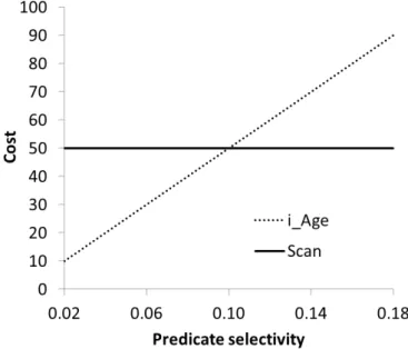
Assume we have a non-clustered index on the attribute Age, call iti_Age. Fig-ure 3.1 shows the costs for scanning the whole table vs using the index i_Age, for different selectivity values. The cost for scanning the table is constant; the cost for using the index increases linearly with selectivity. The two plans intersect when the selectivity =0.1. In order to find out the best access method, we have to estimate the selectivity of the predicateAge < 25, or at least find out whether it exceeds0.1.
Figure 3.1: Cost graph for two plans, table scan and index seek
3.2.0.2 Two-table join
Consider the following join:
SELECT *
FROM Customer C JOIN Order O
ON C.cID = O.cID AND O.Total < 150
There are multiple ways to execute this join. For example, if we consider only the hash-joins, there are two plans possible, shown in Algorithms 1 and 2.
Algorithm 1:Hash join of Customers and Orders H = Filter(Customers, Predicate: T otal <150)
HashJoin(H, Orders, JoinCondition: H.cID=Orders.cID)
Algorithm 2:Hash join of Orders and Customers
HashJoin(Orders, Filter(Customers, Predicate:T otal <150), JoinCondition:
H.cID =Orders.cID)
The difference between Algorithms 1 and 2 is the order of the join. In 1, we first filter the Customers relation and use it as the build input. Namely, the algorithm uses it to build a hash table. The relationOrdersis then probed for matches. In contrast, Algorithm 2 uses the relationOrdersas the build input and the filteredCustomers
relation as the probe input. Now assume for simplicity that the there are no indexes defined on bothCustomersandOrders. Then, the best strategy is to choose the smallerrelation as the input. This means, the optimizer has to assess the cardinality of the expressionFilter(Customers, Predicate: "Total < 150"). Note that in this example we limit ourselves to only one join method, and we exclude indexes from consideration. This shows that even when the execution-plan search space is very limited, selectivity estimates are still needed to find out the better plan.
3.2.0.3 Multi-table join
Consider the join query:
SELECT * FROM Customer C join Order O
On C.cID=O.cID JOIN LineItem L ON O.oID=L.oID WHERE L.Category = "Game"
The following join orders are possible:
P1 = (C1O)1σ(L) P2 = (σ(L)1O)1C
(3.3)
andσ(L)is short for
Filter(LineItems, Predicate: Category = ’Game’).
Each of the plans P1 and P2 are "logical" plans, in the sense that they map into
multiple physical execution plans depending on which physical operators we choose. For instance, σ(L)1O can be carried out using hash join, merge join, and the filter
σ(L)can be implemented by scanningLor by using an index. The costs of all these plans depend on the selectivity of the filterσ.
We will demonstrate this using a very simplified scenario. Assume our only opti-mization goal is to have a result size as small as possible after the first join. In this case, we want to compare the size ofC1Oandσ(L)1O. First, note that
3.2. SELECTIVITY AND CARDINALITY
|C1O|=|O|
This is because each order has one customer. This constraint can be expressed using foreign keys and be made available to the optimizer.
Each lineitem belongs to one order, so
|σ(L)1O|=sel(σ)· |L|
Now, in order to find out whether P1 orP2 is the best plan, we have to compare
|O|tosel(σ)· |L|. Thus, optimal plan choice depends on accurate estamation of the selectivity ofσ.
We demonstrated that in order to estimate the costs of the query plans accurately, the optimizer need to know the selectivity of the query predicates. The selectivities of predicates are crucial in estimating the cost access method of the a single relation, the join method for two relations or the join order of multiple relations. Thus, we have established that we need accurate selectivity estimates in variety of scenarios to ensure effective query optimization.
3.2.1 Properties of Selectivity Estimates
The selectivity of the predicate is the portion of the tuples from the base relation which satisfy the given predicate (see Definition 3). Now consider a predicateπand the random variableXπ, defined as follows:
Xπ = 1, π(t) = true 0, otherwise
The probabilityP(Xπ = 1)is the probability that a randomly selected tuple satis-fies the predicateπ:
Observation 3.1: The probability that a randomly selected tuple satisfies a predicate
πequals the selectivity ofπ.
P(Xπ = 1) =sel(π)
2
This observation allows us to look at the notion of selectivity from the probability point of view. In the following, we will sometimes writeP(π)instead ofP(Xπ)for
improved readability.
Property 3.1: (Selectivity Range)
Property 3.2:(Negation selectivity)
For and arbitrary predicateπ, the selectivity of the negation¬πis given by
sel(¬π) = 1−sel(π)
Property 3.3:(Filtering property) For arbitrary predicatesπ1andπ2,
sel(π1)≥sel(π1∧π2)
The filtering property indicates that applying an additional condition (connected by "and") can only lower the selectivity.
Definition 3.4(Predicate dimensionality)
The dimensionality of the predicate is the number of attributes it refers to. 2
Example 3.3: Revisiting Example 2, let’s compute the dimensionality of the predi-cates:
1. SELECT * FROM Cars WHERE Maker = ’Volkswagen’
The predicate refers to only one attribute –Maker, thus its dimensionality is 1.
2. SELECT * FROM Cars WHERE Maker = ’Peugeot’
Same as above.
3. SELECT * FROM Cars WHERE Maker = ’Peugeot’
AND Year < 1960.
In this case the predicate refers to two attributes, thus its dimensionality is 2.
The predicates that refer to only one attribute are calledunidimensionalor single-dimensional. The predicates that refer to more than one attribute are called multi-dimensional.
3.2.2 Query types
So far, we have not put any restrictions on what kind of boolean predicates the queries can have. Most database systems in fact support a fairly generic class of query pred-icates. However, the vast majority of the predicates that are used in actual queries
3.2. SELECTIVITY AND CARDINALITY
come from a narrow class. As a consequence, most optimizers are most efficient when they encounter predicates from these classes.
Definition 3.5(Range predicate and range query)
A query predicate on relationR(A1, . . . , An)is a range predicate if it has the form π= (c1 ≤A1 ≤C1)∧(c2 ≤A2 ≤C2)∧. . .∧(cn≤An≤Cn) (3.4)
whereciandCiare constants for alli= 1, . . . , n. A query that has a range predicate
is called a range query. 2
The predicate of a range query spans a hyper-rectangle in the attribute-value space.
Example 3.4: Consider the relation Employee(ID, Age, Income) and the query
SELECT * FROM Employee
WHERE Income BETWEEN 25000 AND 45000 AND Age BETWEEN 20 AND 30
The dimensionality of the query predicate is 2.
Figure 3.2: The range query as a rectangle in the two-dimensional space
The query predicate spans a rectangle in the two-dimensional attribute-value space, shown in Figure 3.2.
Note that Definition 5 indicates that the query predicate has to refer to all of the attributes of the relation, while in our example we have omittedID. This is not prin-cipal because our query is equivalent to
SELECT * FROM Employee
AND Age BETWEEN 20 AND 30
AND ID BETWEEN minID AND maxID
Using this trick we can model anyn−kdimensional predicate via ann-dimensional
predicate.
Definition 3.6(Point query)
A point query is a special case of the range query, whereci =Ci for alli= 1, . . . , n. 2
The distinguishing feature of the range queries is that they use constants to define the predicate range. In contrast, the following query:
SELECT * FROM A, B WHERE A.ID=B.ID
does not use constants but rather another attribute for the equality. Such queries are join queries.
Complex queries usually join several tables together and contain range predicates for filtering the some of the individual tables.
Example 3.5: The query
SELECT *
FROM Customer C JOIN Order O
ON C.cID = O.cID AND O.Total < 150
is a join query which has a range sub-query. The sub-query is equivalent to
SELECT * FROM Orders WHERE O.Total < 150
In this thesis, we focus on selectivity estimation of range predicates.
3.3 Requirements for Selectivity Estimation
Selectivity estimation needs meet several criteria in order to be effective. Here, we discuss such requirements.
If the estimates are not precise enough, the estimated and the real costs of the plans will differ significantly. Optimization will become pointless.
Requirement 3.1:(Precision)
Selectivity estimates need to be precise.
Recall that the number of possible execution plans can be rather large even for rel-atively simple queries [RH05]. This means the selectivity estimation subroutine need
3.3. REQUIREMENTS FOR SELECTIVITY ESTIMATION
to be invoked multiple times for a single query. It is clear that selectivity estimation need to be very fast; otherwise the time spent for optimizing a query can become comparable to query execution time.
Requirement 3.2: (Speed)
Selectivity estimation need to be fast, as it it takes place in the inner loop of the optimization cycle.
Usually, selectivity estimation is based on some summary representation of the data. If this summary is large, it needs to be stored on a secondary storage. One should avoid this if one wants to fulfill the Requirement 2: after all, reading from the secondary storage is one of the most time-consuming operations. Thus, we want to keep the size of auxiliary data structures used for selectivity estimation small, such that we can keep the whole thing in main memory. Most systems allocate only several disk pages for these data structures, and pin these pages in the main memory. Pinning means the pages are marked to prevent the system from dumping those pages into the secondary storage. This is similar to what happens to the top level pages of an index. Note that these several disk pages are allocated for the whole database not for a single table or column.
Requirement 3.3: (Space)
The auxiliary data structures used for selectivity estimation need to be compact. The data that the users choose to store in databases can be large and complex. The structure, the volume and the distribution of the data can change over time. In the majority of the cases, the database management systems is supposed to be able to cope with any data which fits the schemata. The system usually does not have a prior knowledge about the data.
Requirement 3.4: (Model-Free)
Selectivity estimation should work for a model-free world, where the data that is present is the only data of interest. The data structures used for selectivity estimation should support this world view.
3.3.1 Multi-dimensional Predicates
One of the major challenges for selectivity estimation techniques is the evaluation of multi-dimensional predicates. In this section, we will show that, in general case, multi-dimensional selectivity estimates cannot be derived directly from single-dimen-sional ones. Later in this thesis (in Chapter 4) we will see that the techniques which handle multi-dimensional predicates are much more complicated than those for the single-dimensional predicates.
query
SELECT * FROM Cars WHERE Maker= ’Peugeot’ AND Color=’Red’.
The predicate here is 2-dimensional. We could assume that the attributes Maker
andColorareindependent. In terms of random variables, it is equivalent of saying that the variables X(M aker =0 P eugeot0) and X(Y ear < 1960) are statistically independent. Then, we can write
P(M aker =0 P eugeot0 ∧Color=0 Red0) =
P(M aker =0 P eugeot0)·P(Color =0 Red0) (3.5)
It is clear that the attributesMakerandColorwon’t satisfy the independence as-sumption in general. To see why this is the case, consider the predicate
Maker=’Ferrari’ AND Color = ’Red’.
For some reason, most Ferraris are red, so applying the independence assumption would drastically underestimate the number of red Ferraris! An important observa-tion here is that the kind of dependency of Colorand Makercannot be deduced from the schema.
Using the independence assumption to compute the selectivity of a multi-dimen-sional predicate as the product of single-dimenmulti-dimen-sional predicates can lead to large estimation errors. We formulate the ability to handle the multi-dimensional predicates autonomously as a separate requirement.
Requirement 3.5:(Multi-Dimensional Predicates)
Selectivity estimation should be able to handle multi-dimensional query predicates without relying exclusively on the independence assumption.
3.4 Summary
Declarative queries rely on query optimization to cope with explosive number of possible execution plans. The optimizer in turn needs selectivity estimates of query predicates.
The selectivity estimates need to be precise, fast, compact and model-free. For multi-dimensional predicates, meeting these requirements becomes particularly chal-lenging. In Chapter 4 we will introduce data structures and algorithms which attempt to solve this problem.
4 Histograms
Abstract. In the previous chapter we talked about the importance of selectivity esti-mation in databases. We also outlined certain properties that the selectivity estimates should have.
In this chapter we review histograms, which are the most commonly used data structure for selectivity estimation. As the literature on histograms is too large, we present only select techniques here.
Parts of this chapter closely follow [?], which has a novel way of categorizing histograms. We consider this categorization to be very clear and effective and decided
to stick to it (with minor changes). 2
4.1 First Histograms
Histograms are a summary representation of data. [Ioa03] points out that they were used as early as in 18th century.
Histograms have multiple uses in databases and related applications. In this chapter we will have in mind a selectivity estimation scenario. In Section 4.8, we will discuss several other applications of histograms.
For better understanding, we discuss the first histograms not on relational data but using the simplest statistical model where the data is a one-dimensional array. Later we return to the relational model. We will start with the simplest histogram, the Equi-Width [Koo80] histogram.
4.1.1 The Equi-Width Histogram
Let the data distribution be
D={0.8,1.1,1.2,2.2,3.3,4.5,4.6,4.88,5.9} (4.1) The Equi-Width histogram partitions the data into ranges of equal width. The his-togram stores the object count for each partition. A value-range together with some statistics is usually called a bucket (we give rigorous definitions later). Figure 4.1 shows a histogram with 6 buckets.
Assume we want to estimate the number of objects in the range[1,1.5]. We know there are two objects in the range [1,2]. The most natural way of approximating
Figure 4.1: An Equi-Width histogram with 6 buckets
Figure 4.2: An Equi-Width histogram with 3 buckets
the number of tuples in [1,1.5] would be to assume that two values are distributed "uniformly" within the interval, which would mean one of them would fall in[1,1.5]. Looking at the data, we can that the actual number of tuples is 2.
Figure 4.2 shows the case when we use three buckets in the histogram instead of six.
4.1.1.1 A disadvantage of the Equi-Width histogram.
The Equi-Width histogram partitions the data distribution into buckets of equal width. When the data is clustered in a small section of the domain, this partitioning can be very suboptimal. Consider the following data points:
C ={5.01,5.02,5.03, . . . ,5.49,5.50}
If we consider the distributionD0 = D∪Cand build a Equi-Width histogram with six buckets, we will see the problem. We added 50 data points to the bucket[5−6). Now, if try to estimate the number of tuples in[5.6,5.9)we will get a the estimate
0.3·50 = 15data points when in fact there is only one data point in that range (5.9). The reason for this large error is that we grouped the ranges [5.0-5.5] and (5.5-6) into one bucket. Those ranges have very different densities and "mixing" them will result in high estimation errors.
4.1. FIRST HISTOGRAMS
It is clear that for better estimations we would have to split the bucket[5−6)into two, and merge some buckets elsewhere. It is also clear that by adding more points into a part of the bucket like we did with merging distributions D and C, we can make the estimation error within that bucket arbitrarily large.
4.1.2 The Equi-Depth histogram
An significant improvement over the Equi-Width histogram was the Equi-Depth his-togram [PSC84]. The Equi-Depth hishis-togram partitions the data into buckets so that each bucket contains approximately the same number of tuples. Thus, if in the Equi-Width histogram the widthof the buckets is fixed, in the Equi-Depth histogram the heightor thedepthof the buckets is the same. Revisiting the distributionD(4.1), the Equi-Depth histogram with three buckets is shown in Figure 4.3.
Figure 4.3: An Equi-Depth histogram with 3 buckets
The advantage of the Equi-Depth histogram over the Equi-Width histogram is that, for fixed amount of data points, it allocates fixed amount of memory to summarize those data points. If the data distribution is very dense for some small range, the his-togram will divide this range and achieve a good approximation of the dense region, unlike the Equi-Width histogram .
4.1.3 Histograms On Relational Data
So far we have looked at examples of histograms where the data distribution is a one-dimensional array. This point of view is common in statistics, where the data is simply a sample from the (unknown) probability distribution. Contrary to this, relation model organizes data into tables.
There are several models on how to build histograms on relational data. Here we describe the model which is widely used because its aim is to assist cardinality estimation in databases. In this model, the data can be viewed a set of pairs
S ={(vi, f(vi))|1≤i≤N} (4.2)
where vi is the attribute value and f(vi) is the frequency – the number of times it
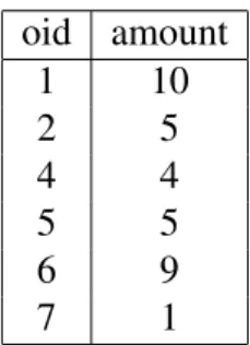
drawn from[0, M]. Table 4.1 shows a table with two columns, order-id (oid) and amount. When building a histogram on the attribute "amount" our set of pairs will be
oid amount 1 10 2 5 4 4 5 5 6 9 7 1
Table 4.1: Orders table with order-id and amount of order
(10,1),(5,2),(4,1),(9,1),(1,1)
We discussed in Section 3.2.2 that there are two general types of selectivity es-timation problems. Those are the join and the range-query selectivity estimation problems. We are going to focus on the range queries mostly. This means that we want the histogram to approximatesumsoff(vi)values for some consequent values
ofi. Given a set of values S as in 4.2, the goal of the histogram is to approximate sums of form
σ(r) =X
i∈r f(i)
ris a range predicate, i.e.r={j, j+ 1, . . . , j+k}for somej andk.
In order to estimate range-query cardinalities, histograms divide the data into buck-ets.
Definition 4.1(Bucket)
A histogram bucketb is pairb = (r(b),Ω(b)), where r(b)is a subset of[0, M], and
Ω(b)is some aggregate information about tuple frequencies within that subset. 2
The setr(b)often represents a range. The statistic to store in the histogram bucket,
Ω(b), is key for issuing selectivity estimates. In the simplest case, Ω(b) is simply the average frequency within the bucket. Clearly, it is possible to store more detailed information, which increases the memory footprint of a bucket. Thus, the choice of information to store in a bucket is a compromise: storing detailed information means we can approximate the in-bucket distribution better at the cost of having less buckets overall. The Equi-Width histogram divides the data into near-equal ranges. So the rangesr(bk) = r(bk+1). The statistics stored is
Ω(bk) =
X
i∈r(bk)
4.1. FIRST HISTOGRAMS
The Equi-Depth histogram divides the data into so that they have equal nearly amount of tuples in them, i.e. Ω(bk) = Ω(bk+1)for all buckets except maybe the last
one.
Both histograms use the the Continuous Value Assumption to approximate the data distribution within a bucket.
Definition 4.2(Continuous Value Assumption )
Under the Continuous Value Assumption , the number of tuples that lie within the query interval is assumed to be the fraction of bucket range that lies within the inter-val multiplied by the bucket count. Formally, if query range isq, then
count=n(b)· |q∩r(b)| |r(b)|
2
Basically, the Continuous Value Assumption says that the density withing the bucket is uniform.
We already demonstrated the Continuous Value Assumption when estimating the cardinalities in Sections 4.1.1 and 4.1.2.
4.1.4 Histogram Categorization
So far we have seen that the Equi-Width and the Equi-Depth histograms arrange the buckets in the different manner, but they use the same method to approximate the distribution within a bucket.
It turns our that most histograms out there can be categorized regarding how they divide the data into buckets, what kind of statistic they store, how they approximate frequencies given a bucket information and so on. This kind of categorization helps understand how different histograms relate to each other, and what is their principal differences are.
The following aspects of histograms can be used to categorize them:
• Bucketing scheme. The Equi-Width and Equi-Depth histograms use disjoint, continuous ranges for buckets. As we know from Definition 1, buckets can be an arbitrary grouping of attribute values. Some histograms use overlapping or recursive bucketing schemes.
• Statistics stored.The Equi-Width histogram stores the number of tuples in the bucket, while the Equi-Depth histogram stores the bucket boundaries. Some histogram variants store number of distinct values or the variance of the fre-quencies of tuples in the bucket.
• Approximation scheme.So far we have mentioned only the Continuous Value Assumption as tuple-count estimation scheme. The approximation scheme de-pends strongly on the statistics stored in the buckets. Usually, the more aggre-gate information a single bucket contains, the more evolved the approximation scheme can be.
• Class of queries answered.Histograms are used to estimates the selectivity of range,point, andjoinpredicates. Joins and range queries can use different data structures for selectivity estimation. Most of the histograms discussed here aim for range queries, however we mention several join-friendly histograms as well.
• Incremental Maintenance. Data in the database changes, and the histograms need either to be rebuilt periodically or allow incremental maintenance. In-cremental maintenance can be important in the case when the data changes rapidly, or the building cost of the histogram is relatively high. This is espe-cially relevant for multi-dimensional histograms, where the construction costs are typically high.
• Misc. Other features include error guarantees, size, build time etc. These are important issues but are somehow beyond the scope of this thesis, and we refer the reader interested in these issues to respective papers.
4.2 Estimation Schemes
The estimation scheme is the the method of estimation of the frequencies within a bucket.
4.2.1 Equi-Distant Schemes
The schemes described here are more commonly referred to asUniformschemes in the literature, which is a rather inappropriate term. We will stick to the term "Equi-distant" here.
Equi-distant schemes store the number of tuples with non-zero frequency in the bucket, together with the total number of tuples.
Let {b1, . . . , bm} be disjoint histogram buckets, each bucket representing an
in-terval, so that the union of all bucket intervals covers the whole data range. An equi-distant scheme stores the number of tuples in the bucketn(bj)and the number
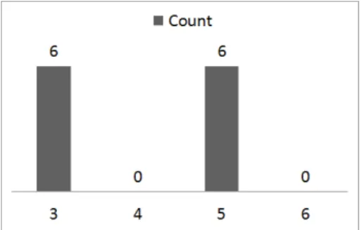
of non-zero values in the bucket,s(bj). Figure 4.4 shows a distribution with where
two out of four values have positive frequency.
4.2. ESTIMATION SCHEMES
Figure 4.4: A sample distribution
Figure 4.5: An Equi-Depth approximation of the distribution using a single bucket.
Figure 4.6 shows a histogram on the same data, this time using the Equi-distant approximation scheme instead of the Continuous Value Assumption . The histogram stores the number of positive values and the average frequency. It approximates fre-quencies assuming the positive values are distributed equi-distantly in the bucket.
Figure 4.6: An Equi-distant approximation of the distribution, using 1 bucket with 2 non-zero values.
The Equi-distant estimation scheme is often used for JOIN and aggregation que-ries. The study in [WS08] shows that the Continuous Value Assumption usually outperforms the Equi-distant approximation scheme, both for single-dimensional and multi-dimensional data.
4.2.2 Other Approximation Schemes
Splines. The Continuous Value Assumption approximates the tuple frequencies within a bucket with a constant (the average). A natural generalization of this is a spline-based scheme where, for instance, the bucket stores two values instead of one and uses a linear function to approximate the densities. Indeed, it is possible to further enhance this by using polynomials. We refer to [KW99, ZL02, ZL96] for further reading.
Multi-Level Trees. 4-level trees (4LT) and n-level trees [BL04, BLS+08] are
hi-erarchical bucketing scheme for enhancing the precision of the histogram. We briefly explain the 4LT [BLS+08] here, as it aims for a compact representation which al-lows to store the auxiliary information in one 32-bit or 64-bit integer. The idea is to store approximate partial sums of the elements that fall into the bucket. We can think of sub-buckets which can overlap and contain approximate rather than exact information. Assume we have 16 values,v1, . . . v16, that we want to store in a bucket.
The bucket is divided intoj segments of equal length, and the sum of the values of thei-th segment is denoted byσi/j. The sum of all the values in the bucket, σ1/1 is
stored exactly (that’s the first level). The second level contains the σ-s for j = 2, the third level corresponds toj = 4and the fourth level corresponds toj = 8. The number of bits allocated to each level is different as well. For j=2, 4LT allocates 6 bits for theσi/2, for j=4 its 5 bits, for j=8 only 4 bits. Such a storage of partial sums
forms a tree. There is no need to store allσi/j for all i, j. Notice that for instance σ1/1 = σ1/2 +σ2/2, and we have the exact value forσ1/1, so if we store sayσ1/2 we
can computeσ2/2 from those values. The same applies to the rest of the tree too. 4LT
stores 1 value for j=1, 1 value for j=2, one 2 values for j=4 and 4 values for j=8. This makes 32 bits. For the exact approximation scheme and more detail, see [BLS+08].
Combined Schemes. From all schemes mentioned above there is not one which is universally the best. [WS08] exploits the fact that different bucketing schemes can in fact be better for different datasets. In essence, it uses either 4LT, the Continuous Value Assumption or the Equi-distant schemes for different buckets. The overhead is that the histogram has to store descriptors about the scheme used. The experiments in [WS08] show this approach outperforming all "fixed" schemes, however, we would like to mention that the authors dedicate uncommonly large amount of memory for the histogram (5% of the data set).
4.2.3 Bucketing Schemes
So far, we have discussed the Equi-Width (Section 4.1.1) and the Equi-Depth (Sec-tion 4.1.2) bucketing schemes. Multi-level trees such as the 4LT and nLT deploy a
4.3. STATIC MULTI-DIMENSIONAL HISTOGRAMS
hierarchical bucketing scheme. In the following, we discuss several other bucketing schemes which we haven’t encountered so far.
4.2.3.1 Singleton Schemes
Singletonbucketing is used mostly for data where several of the most-frequent values fill almost the whole dataset. For instance, End-biasedhistograms storeh elements with highest f-value and l elements with lowest f-value in singleton buckets. The rest of the data is assumed to be uniform and is allocateds−(h+l)buckets, where
s is the overall memory budget [IC93, Ioa93]. High-biased histograms have l = 0, i.e. they store only the high-f values. Similarly,Low-biasedhistograms haveh = 0. Compressed histograms [Ioa93] combine the High-biased and Equi-Depth his-tograms. They store the helements with the highest f-values in singleton buckets. For the rest of the data range, they construct an Equi-Depth histogram.
4.2.3.2 MaxDiff Histograms
Maxdiff histograms draw the bucket boundaries where there is the highest frequency difference between f-values. Thus, if the histogram bucket budget is B, the data range is[1, M], then there is a bucket boundary betweeniandi+1of|f(i+1)−f(i)|
is among theB −1largest such differences. Maxdiff histograms require sorting the whole dataset in order to obtain the largestf-values. In practice, the cost for sorting is usually inacceptably high; for this reason Maxdiff histograms are usually constructed using a sample.
4.3 Static Multi-Dimensional Histograms
One of the requirements on selectivity estimation was that the multi-dimensional predicates need to be evaluated without relying on the independence assumption (Re-quirement 5 in Section 3.3.1).
In order to achieve this we need data summaries which can capture the joint data distribution of multiple attributes. Multi-dimensional histograms are a prominent representative of such summary structures.
Not surprisingly, first multi-dimensional histograms were generalizations of known one-dimensional approaches for multiple dimensions. Namely the method in [MD88] attempts to obtain a multi-dimensional Equi-Depth partitioning of the data. It starts with one bucket containing whole data. In each step, an existing bucket is split across a dimension, and this is repeated for all dimensions.
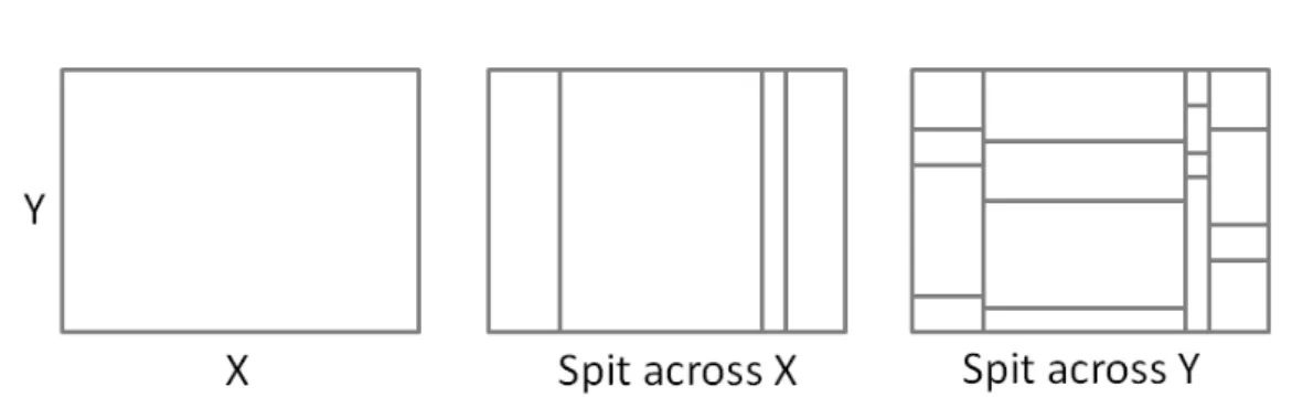
Figure 4.7 demonstrates the process for a 2D case. At first, the histogram contains a single bucket, which is the whole dataset. Then, a split dimension is chosen (in our example the X-axis) based on one-dimensional statistics, and the histogram is split
Figure 4.7: Creation of a multi-dimensional Equi-Depth histogram
across that dimension. The number of buckets created at each split step is fixed, and chosen so that in the end the number of buckets meets the space budget. As in the single-dimensional case, the buckets are created so that they contain approximately even number of tuples. Then, this step is repeated for each remaining dimension. So each bucket is split into four across dimensionY this time, again trying to preserve equal number of tuples inside the buckets.
The problem with the multi-dimensional Equi-Depth histograms is that the princi-ple of making buckets with fixed number of tuprinci-ples is inefficient, at least when cou-pled with the Continuous Value Assumption . If the Continuous Value Assumption is used, it seems clear that the buckets should resemble data regions with close to uniform distribution of tuples.
[PI97] attempts to solve this problem, pointing out that the underlying uni-dimen-sional histograms do not have to be Equi-Depth . They propose a generalization of the histograms introduced in [MD88]. Their approach is coined MHist and takes MaxDiff(v, a)(see [Ioa03]) uni-dimensional histogram instead of the Equi-Depth his-togram. TheMaxdiff(v, a)histogram attempts to minimize the variance of tuple fre-quency within the bucket.
GENHIST histograms [GKTD00] allow buckets to overlap. If a region lies within an intersection of two buckets, the density is the sum of densities of the buckets. GENHIST starts with a grid of cells over the data set, which is typically fine-grained. The algorithm then merges dense cells into buckets and removes the tuples that fall within that bucket from the dataset. This step is repeated with the new dataset (with tuples removed), this time with a coarser initial grid. The GENHIST algorithm results in good histograms, but the construction costs are restrictively high. The RK-Hist histogram [EL07] also uses intersecting buckets, resembling an R tree. First, a Hilbert curve is fitted into the data space. Then, the tuples are sorted according to their appearance along the curve. Buckets are formed so that close tuples are in the same bucket.