UNIVERSITY OF TARTU
FACULTY OF MATHEMATICS AND COMPUTER SCIENCE
Institute of Computer Science
Jevgeni Võssotski
SAR Image Denoising Using Non-Local
Means on MapReduce
Bachelor’s Thesis (6 ECTP)
Supervisor
:Pelle Jakovits, M.Sc.
SAR Image Denoising Using Non-Local Means on MapReduce
Abstract:
Satellite systems designed for exploratory surface scanning face the problem of noise presence in images acquired electromagnetically, i.e by means of radars. A solution to this inherent problem has been searched for in the area of noise reduction filters applicable after the raw data is collected. The filtering algorithm Non-Local Means had shown to give good refinement results. However, the method is known to be computationally expensive, which poses a problem for processing of large datasets. In this work the parallel computing approach to this task was implemented on the distributed processing framework Apache Hadoop. It was shown that the Non-Local Means approach to noise reduction problem can be successfully adapted for execution in the distributed fashion of MapReduce model. Benchmark experiments were carried out on the test image to evaluate scalability of the approach. Tests confirmed high efficiency of parallelization (16 executor setup had given a speedup of 13.14×) and showed positive potential of Hadoop as a platform for massive image processing.
Keywords:
synthetic aperture radar, SAR, radar imaging, image denoising, NL-means algorithm, Apache Hadoop, MapReduce, parallel computing, distributed computing.
Müra eemaldamine SAR piltidelt kasutades NL-means
algo-ritmi MapReduce mudelil
Lühikokkuvõte:
Maapinna skaneerimise ja uurimisega tegutsevate satelliitide süsteemide üheks suureks probleemiks on müra, mis esineb elektromagnetiliselt (i.e. radarite poolt) saadud piltidel. Selle probleemi lahenduse üheks suunaks on müra vähendamise filtrid, mida rakendatakse töötlemata andmetele. On tõestatud, et filtreerimisalgoritm Non-Local Means annab väga head filtreerimistulemused. Seevastu aga on teada, et see algo-ritm nõuab suurt arvutusvõimsust. Käesolevas töös sellelle probleemile lähendatakse paralleelarvutuse metoodikaga hajusarvutuse raamistiku Apache Hadoop abil. On näi-datud, et müra vähenemise meetodit Non-Local Means saab edukalt adapteerida käivi-tamiseks MapReduce hajumudelina. Meetodi skaleerimise hindamiseks on läbiviidud eksperimendid testpiltidega. Need katsed kinnitavad meetodi kõrget efektiivsust (16 protsessoritega klastri puhul on saavutatud 13.14× kiirendus) ja näitavad platvormi Hadoop positiivset potentsiaali piltide massiliseks töötlemiseks.
Võtmesõnad:
tehisavaradar, SAR, Müra eemaldamine, pilditöötlus, NL-means algoritm, Apache Hadoop, MapReduce, paralleelarvutused, hajusarvutus.
Contents
Abstract . . . 2
Introduction . . . 4
1 Background 6 1.1 MapReduce programming model. . . 6
1.2 Hadoop as a MapReduce execution framework . . . 7
1.2.1 HDFS . . . 8
1.2.2 Hadoop MapReduce . . . 9
1.2.3 Data serialization in Hadoop . . . 11
1.3 Synthetic Aperture Radar (SAR) . . . 12
2 Proposed solution 14 2.1 Image processing with MapReduce . . . 14
2.2 Image filtering with Non-Local Means. . . 16
2.3 NL-means algorithm implementation in Java with MapReduce . . . 20
3 Validations 24 3.1 End-to-end process overview . . . 24
3.2 Testing environment and dataset . . . 25
3.2.1 Test results for sequential parts . . . 25
3.2.2 Parallel execution test results . . . 25
3.2.3 Comparison to non-parallel execution . . . 26
3.3 Amdahl’s prediction . . . 28
3.4 Conclusions . . . 28
Introduction
On the 4th of October 1957 a successful launch of “Sputnik 1”, the first man-made Earth satellite, took place at Baikonur Cosmodrome. Since that day numerous satel-lites have been launched into orbit of our planet, their projects targeting a wide range of purposes.
Nowadays the applications of satellite-based explorations become ever more ver-satile. For instance, as part of European Commission’s Copernicus programme there has been recently1 launched satellite Sentinel-1 by European Space Agency. One of
its proposed missions is to collect the terrain images of large cities throughout time to provide analytical data of urbanization rates and various land usage characteristics. It is also capable of providing data that allows to monitor land surface motion risks.
Terrain images acquired from satellite radars are affected by different unwanted side-effects that in one or another way degrade reading of data they provide. As an example from optical imaging, a photograph may suffer from misplaced white balance, which results in unnatural colors. Post-processing methods are developed to mitigate such negative effects. Our area of interest is the side-effect of a noise typical to data supplied by radars — the so-called “speckle” noise that appears when the reflected signal is coherently collected from multiple distributed targets. We refer to the process of noise reduction as filtering ordenoising.
In this work we examine images obtained from a special type of radar — synthetic aperture radar (SAR) — as they are commonly used for land surface scanning.
For this purpose we will choose a denoising algorithm called Non-Local Means. This algorithm tries to correct values of an image by looking at neighborhood pixels and evaluating similarity of patterns surrounding the pixel under examination. As a result a noise-free estimate of examined pixel’s value is given in a least biased way.
Our goal is to adapt the chosen denoising method to be run in a distributed fashion and try to estimate the efficiency of parallel execution. As a platform of distributed computations for this work we chose the Hadoop framework, which allows to employ MapReduce approach as means to divide problem into subproblems of smaller size. MapReduce is a technique allowing to process large data sets on cluster of multiple nodes. To utilize it an algorithm must be broken down into 2 steps (Map and Re-duce) and follow their contracts in terms of input data partitioning and output data aggregation. Operations that are orthogonal to solving the problem at hand (such as load-balancing, data transfer, fault resilience, etc.) are handled by the Hadoop system. In a single-process driven implementation the denoising of large images may be limited by the amount of main memory available to the executor process. This is one of problems that can be successfully solved by partitioning the input. Other benefits provided by parallel execution are of interest as well, e.g. vertical scalability — achieving higher throughputs by adding more parallel executors. Particular benefits of distributed execution as well as general requirements and specific considerations for the approach will be described in chapter 1.
Given a range of potential improvements, we assume that the above mentioned denoising solution can be implemented as pleasingly parallel 2, meaning that it can
run in a distributed manner with no significant overhead (as compared to a
non-1on 3 April 2014
parallel execution). Due to specifics of algorithm, a trivial split-and-merge is not enough, namely the split phase must be enhanced to keep the method accurate. This is discussed more precisely in chapter 2.
Finally we conduct a series of tests (described in chapter 3) that are supposed to support or refute the main hypothesis — that the image denoising problem of large images is a good candidate for implementation as a MapReduce program, both from resulting performance and implementation simplicity standpoints. This might be particularly useful for work with radar images, since their sizes may be enormous, and they may also require computationally expensive post-processing similar to the one considered in this work.
Thesis is organized as follows:
Chapter 1 provides background information about the stated problem and settings it was solved in: SAR principles, MapReduce approach and Hadoop architecture and mechanics are introduced in this chapter.
Chapter 2 gives the description of the denoising algorithm used for this work, as well as means to adapt it for execution on the MapReduce platform.
Chapter 3 gives results of tests performed on a sample image, and also analysis of the scalability characteristics of used solution.
Chapter 1
Background
1.1
MapReduce programming model
MapReduce is a distributed computing model designed to process big data sets on multiple computers by dividing the data between them to utilize potentially large number of workers. Thus the data processing load is distributed between computers, or nodes, that are collectively referred to as cluster.
The model prescribes two main phases: MapandReduce, the former being respon-sible for processing a subset of input data and the latter for folding or aggregating the results of Mapphase. The fraction of input data assigned to each Map function is often called a “split” [e.g.DG08]. Both steps are driven by user-defined functions that encapsulate domain logic of the problem. There is also an intermediate step, carried out by the MapReduce library, that stores and groups results of Map function and passes them to Reduce function. The result of Reduce phase is stored on the cluster and can be used by the master node to form the solution of stated problem or can be used as an input to another MapReduce job. A job consists of as many Map and Reducetasks, i.e. scheduled and tracked executions, as required for all the input data to be worked through.
Map function supplied by user accepts (key, value) pair of key and value and produces one or more (key, value) pairs, though the types of input key/value can be (and often are) irrelevant to types of output key/value. In short, this can be expressed as follows:
M ap: (K0, V0)→list[(K, V)]
Output provided by Map worker (node assigned for invocation of Map function for a particular input split) compose intermediate result set of key, value pairs. Values of intermediate results that are associated with equal keys are then grouped together by MapReduce framework into set of pairs (K, list[V]), and these form input for the Reduce function. Thus the Reduce, also a user-specified function designed to merge together intermediate results, has the following form:
Reduce: (K, list[V])→list[(K, V)]
Typically a Reduce function would return one or no result value, this way the overall output of MapReduce job would contain at most one result for each key. Note that since outputs of Reduce invocations constitute the final result of the job, Reduce
workers can start their job no sooner than all intermediate results are received, i.e. when there are no more unprocessed input splits left.
As an example let’s consider the task of creating a simple inverted index of words used in a collection of text documents. For such task the map function would be:
revIndex: (documentN ame, documentContents)→list[(word, location)] ,
where “location” can be defined as the document name and the number of line where the word occurred. Intermediate results would contain set of locations for each word in every input document. For our example the reduce function will be as trivial as the identity function, since all we need is to get a list of occurrences for a word, which is already achieved by grouping intermediate results.
The MapReduce model aims to improve the work on large amounts of input data through the following principles:
• A large set of data is processed iteratively. This means, for instance, that the Map function should not be responsible for storing intermediate results on a disk, furthermore, it can emit intermediate results (key, value) one-by-one as soon as they are computed, which can lower memory requirements for the algorithm. On the other hand, Reduce function operates on intermediate values in an iterative manner as well, thus allowing to handle arrays of data that are too large to fit in memory all at once.
• The user is only required to write map and reduce functions in terms of data types and transformations relevant to the task at hand, while the MapReduce library is responsible for all the data interoperability and execution control. This means that the program is more task-oriented and less of irrelevant code needs to be maintained.
• The library is also responsible for handling machine failures of a node in a grace-ful manner. This is achieved by keeping input/output data persistent and by rescheduling failed batches of work, thus making the process more result-oriented. This feature of fault-tolerance is also orthogonal to problem solution logic, mean-ing that Map/Reduce functions do not need to recover failures or keep track of status of invocation.
1.2
Hadoop as a MapReduce execution framework
Though it is possible to execute MapReduce model on a single machine having multiple cores as processors, this approach is commonly used in a networked environment of loosely coupled computers, as it brings even more benefits which are described further in this chapter. In this work we will examine Hadoop – an open source implementation of MapReduce developed by the Apache Software Foundation.
Hadoop is a project delivering a set of systems and client-server applications built to fulfill a wide range of distributed computing needs. It was chosen as a target platform for several reasons:
• it has a large user base and is widely adopted in industry as well as in academics [see ASF14];
• its code is open-sourced and its license allows free usage;
• there exist adequate documentation on the side of the maintaining organiza-tion (Apache Software Foundaorganiza-tion) as well as numerous articles and knowledge resources shared by the community of users.
The following components comprising Hadoop platform are of most interest in scope of current work:
• Hadoop Distributed File System (HDFS) – A distributed file system that pro-vides high-throughput access to application data.
• Hadoop MapReduce – an implementation of a MapReduce framework that is easy to adapt and is highly customizable in terms of input and output data format.
Both these subsystems employ master/slave architecture and can work indepen-dently of each other. As a whole, Hadoop is responsible for running the application in parallel flows of execution, while “managing the household” at the same time: taking care of communication between peers, reliable data storage and handling of execution failures. All that is required from the application designer is to create program code that complies with the style of Map and Reduce steps described earlier. Such separa-tion of concerns gives an important advantage, namely that the program does not need to deal with most problems of parallel computing directly, meaning less unnecessary complexity in the solution of task at hand.
1.2.1
HDFS
HDFS is designed as a distributed storage capable to hold large amounts of files on the cluster, providing reliable access to these files by means of data separation and replication between nodes. The system handles all the stored data in blocks of fixed size. E.g. default HDFS block size is 64 MB1 , different sources suggest optimal values ranging from 32 to 256 MB depending on size of cluster. One of implications of block-based organization is that when a file of size twice as big as the block size is put into HDFS, it will be stored in two independent blocks that can possibly make it into two different nodes. Also, a copy of each block is stored on as many distinct nodes as required by the replication factor configured in the system.
Although it is acceptable to store large files (spanning multiple blocks) on HDFS, accessing such file in random fashion would bring down overall performance, so a sequential access must be preferred for such files.
HDFS has a master node, called NameNode, through which clients operate on file system, and one or more DataNodes that store actual data in blocks on their side. Same machine can be assigned roles of NameNode and DataNode at the same time.
From the client’s point of view the access to a file located on HDFS is transparent, as all mechanics required to actually locate and read/write the file are abstracted via HDFS layer. However, the client-server protocol is designed in a way that allows an optimal point-to-point data transferring: whenever possible the data is streamed
1with MB we denote a “large” megabyte, i.e. 1 MB = 220 = 1,048,576 bytes; e.g. 64 MB =
between the client and the DataNode (e.g. containing currently accessed file) directly, meaning that NameNode acts as a controller and no user data traffic is passed through it (unless it also serves as a DataNode itself). This technique is employed for data interchange within cluster as well, e.g. between a storage node and an executor node. MapReduce approach to task solving and HDFS as a data store complement each other: a requirement to have at least few copies of every data block in the distributed file system makes it possible to balance the load of resources in the cluster and to maximize the locality of data.
1.2.2
Hadoop MapReduce
The usual workflow of running a job in a Hadoop cluster is comprised of putting the data into HDFS and submitting the program code to a JobTracker that manages task queues. A JobTracker is responsible for monitoring and control of jobs, and for dispatching of Map and Reduce tasks to nodes serving as TaskTrackers.
A TaskTracker performs tasks on a slot basis. For instance, a TaskTracker can be configured to have 2 slots: at a particular moment one might be running a Map or Reduce task while the other one is being idle and waiting for new tasks from the job tracker. There can be one or more TaskTrackers serving on one machine, but it might be more convenient to set up a single TaskTracker with multiple slots instead.
Figure 1.1: Hadoop cluster setup example, source: Wikipedia[Wik14b]
Usually there is one JobTracker and one NameNode serving on the master node of a cluster Other nodes, often referred to as slave nodes, can act as both DataNodes and TaskTrackers. Figure 1.1 shows scheme of nodes organization.
Optionally the master can act as a DataNode and TaskNode as well. Using this design input and output data of a job are stored on the same set of nodes where task executors are serving – this condition is crucial for achieving data locality, since Hadoop makes use of location information of the files to schedule a Map/Reduce task on a machine that contains a replica of the corresponding input data. Combined with a distributed workload of a job that can provide a high aggregate throughput of application data.
Let us consider the problem of processing a large image (up to several GB in size) in a way that every element of the image (pixel) is examined and possibly altered as specified by the algorithm. By splitting the image into parts and submitting them to Hadoop framework, the application gains the following useful properties:
• Fault-tolerance. Should some Map or Reduce operation fail to complete (e.g. the node goes down due to technical failure), this task can be reassigned to an-other active node, thus allowing the job to execute completely. Hadoop keeps track of parts of input designated to particular nodes and their current status, and is able to recognize a failed task and reschedule it, possibly to another node. Hadoop also has means of detecting slowly running or hung tasks and restarting them as well. On the data access level HDFS also takes care of this by par-titioning files into blocks and replicating them across machines of the cluster, lowering risks of disk failures. This feature is of importance when processing a vast amount of image data because results of already processed parts will not be rendered void by random unexpected errors or failures. Naturally this presumes that for a particular batch of input will eventually complete successfully, other-wise the job is marked to contain unrecoverable errors and the output cannot be considered final nor complete.
• Scalability. Once the cluster is set up it should be easy to add more nodes, that would possibly allow the job to perform better. Hadoop allows the topology of cluster to be changed and new nodes added to the cluster can be utilized by reconfiguring the master node. The program code must not be changed, because it does not depend on the cluster configuration in the first place (still it is possible to programmatically set up job parameters, e.g. to set the maximum number of concurrent tasks for current job depending on the size of the cluster). In context of image processing this flexibility can be useful, because the amount of data and computational complexity can be unknown beforehand.
• I/O load distribution. As the size of input data can, and often is found to be very large, introducing parallelism into data input/output operations can highly increase overall throughput as well, because for a common modern computer I/O operations are much less time-efficient than CPU operations. This feature assumes that the framework is able to ensure a good strategy for input data distribution between executor nodes, in a way that a node gets assigned for pro-cessing a split of data that is stored as close as possible to it. Hadoop MapReduce is able to achieve very good data locality for most tasks, in the sense that most input data is read locally and network traffic between nodes is minimized.
Listing 1.1: "Example of Writable implementation" public c l a s s M e s s a g e W r i t a b l e implements W r i t a b l e { public S t r i n g t e x t ; public L i s t <S t r i n g > r e c i p i e n t s ; /∗ . . . ∗ [ c l a s s c o n s t r u c t o r and o t h e r methods o m i t t e d ] ∗ . . . ∗/ @Override
public void w r i t e ( DataOutput dataOut ) throws I O E x c e p t i o n { dataOut . writeUTF ( t e x t ) ;
dataOut . w r i t e I n t ( r e c i p i e n t s . s i z e ( ) ) ;
f o r ( S t r i n g r e c i p i e n t : r e c i p i e n t s ) {
new Text ( r e c i p i e n t ) . w r i t e ( dataOut ) ; }
}
@Override
public void r e a d F i e l d s ( DataInput d a t a I n ) throws I O E x c e p t i o n { t e x t = d a t a I n . readUTF ( ) ;
i n t r e c i p i e n t s S i z e = d a t a I n . r e a d I n t ( ) ;
r e c i p i e n t s = new A r r a y L i s t <S t r i n g >( r e c i p i e n t s S i z e ) ;
f o r (i n t i = 0 ; i < r e c i p i e n t s S i z e ; i ++) { Text r e c i p i e n t = new Text ( ) ;
r e c i p i e n t . r e a d F i e l d s ( d a t a I n ) ;
r e c i p i e n t s . add ( r e c i p i e n t . t o S t r i n g ( ) ) ; }
} }
1.2.3
Data serialization in Hadoop
Though Java has a built-in serialization mechanism, Hadoop employs a serialization framework of its own. It allows to define custom data types that act as a unit of record being transferred between nodes or made persistent on HDFS. On the pro-gram code level the same data type can be used for input and output of map/reduce methods. Custom data types are supported by Hadoop on the basis of interface
org.apache.hadoop.io.Writable.
A class that needs to make its way into Hadoop’s data flow must implement methods “void readFields(java.io.DataInput)” and “void write(java.io.DataOutput)” in a way that allows to persist relevant object state. This is done by means of DataInput and DataOutput objects supplied as arguments. These provide writing and reading operations for primitive types, such as readLong() and writeLong(), that allow to define serialization of arbitrary data structure. Note that DataInput and DataOutput classes are a part of the standard JRE2 library. Consider an example of a class representing a message in listing 1.1.
When reading from disk, the framework will instantiate newMessageWritable
ject and call the readFieldsmethod on that object. To serialize aMessageWritable
object, the write method will be called. Note that this model of callback methods allows to reuse implementations of other Writable classes, as in the example above a String is read and written usingorg.apache.hadoop.io.Text residing in Hadoop library.
1.3
Synthetic Aperture Radar (SAR)
A typical radar3 system sends beams of radio wave (usually emitted from antenna)
and “listens” for “echoes” that occur when a wave is reflected from an obstacle. This is possible because when a wave encounters an impenetrable material, a part of the wave’s energy continues to travel as a reflection. Radars are often used with the purpose of detecting location or range of an object of interest.
Synthetic aperture radar (SAR)[Wik14d][Key92] is a special type of radar that can be used to obtain information about form and, to some extent, material of target objects. It is usually mounted on a platform moving in the air above the examined area, such as an aircraft or a satellite orbiting the Earth, and is employing a single beam-forming antenna to illuminate the target of interest with pulses of radio waves at wavelengths from a meter down to millimeters. The consecutive motion is a require-ment for SAR, because it is based on the idea of utilizing forward moverequire-ment of the radar itself to get the effect of having a wider aperture — an area capturing reflected waves — this allows to obtain a higher spatial resolution without having to construct an antenna of a large size. The multiple backscattered signals received successively at the different antenna positions are used to put together an image of the target scene, providing data of surface elevations with resolutions of up to 1 cm.
Since said radar uses microwaves (wavelength from meter to millimeters), this scanning method, compared to optical capturing systems, has an advantage of not being affected as much by weather or other environmental lighting conditions.
However, any detection using reflected electromagnetic waves suffers from short-comings due to the fact that backscattered wave is coherently collected from many scattering centers which contribute to response signal. As a side-effect this produces a certain kind of noise, often referred to as speckle, that emerges on the image as ran-dom pixels having an outstanding shift of their value. For instance, when the resulting image is rendered to a monochrome picture, pixels affected by speckle noise stand out as conspicuously bright or dark dots, forming some sort of graininess in general.
Speckle noise is usually interpreted as a random noise, and there are various noise reduction techniques developed to be applied as a separate filtering step during post-processing of an image. Large class of such solutions consists of methods that make use of averaging neighboring pixels (possibly using some weighting strategy as well), thus dispensing the aberration among all pixels of an image, whether or not they have been altered by the noise at all, which as a rule leads to lowering resolution. Most of these filtering methods imply some sort of afilter parameter that is used to control how intensive the denoising process shall be, so the choice can be made between reducing less noise or preserving less details.
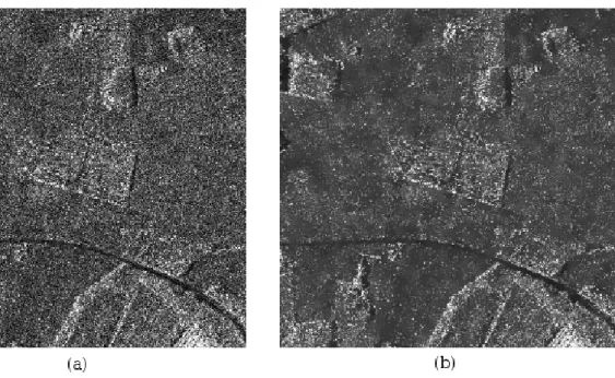
In the current work we will examine how an algorithm called Non-Local Means
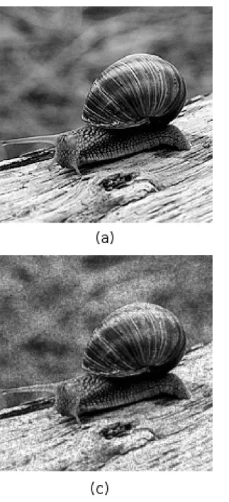
Figure 1.2: Example of (a) speckle noise and (b) the same image after noise reduction (NL-means method implementation developed during current research)
(NL-means) can be used with terrain images containing speckle noise. When applied to SAR data, this method proves to remove noise effectively without notable loss of spatial resolution [DTD10] (see figure 1.2). The difficulty encountered in adapting any sufficiently advanced denoising filter is the enormous amount of data contained in images acquired from a SAR unit. Moreover, the NL-means algorithm at its core is rather expensive with respect to computational resources (see results section for overview of sample run times).
Chapter 2
Proposed solution
2.1
Image processing with MapReduce
In this work we will take images containing noise and process them as input datasets for MapReduce, treating these images as a dense matrix, where each element of the matrix represents the value of the corresponding pixel. Distributed processing of this dataset can be achieved by partitioning the input into set of smaller matrices. Required operations are carried out for each submatrix within the Map step, and depending on the particular task the result is collected within Reduce step. The Reduce phase can be bypassed, for instance if the computation in Map step produces a transformed representation of the original data, e.g. contrast or sharpness correction – this applies to many common image processing tasks, and as well suits the problem of noise reduction that this work is focused on. So in scope of the current problem the Reduce phase will be mostly omitted from consideration.
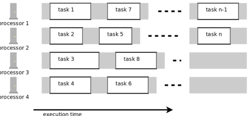
The additional step that needs to be done outside of MapReduce model in order to form a final result (a filtered or transformed image) is the composition of submatrices back into a larger one in the correct order. With respect to this particular scenario, a MapReduce is used as a framework for a distributed form of fork-join strategy[Wik14c], where a task is split into N subtasks served by workers in a cluster and their results are merged back when all subtasks are completed. A simplified representation of parallel task processing is given in figure 2.1.
This also gives the benefit of working with smaller amount of data per task executor, which is important because the potential size of input image can be too large to have it processed in one pass by a single process since the image data cannot fit entirely into memory owned by the program running the algorithm. Alternatively the algorithm itself could be modified to cope with large input data, but that would introduce unnecessary complexity which would rather be abstracted from the image processing logic.
A simplified method of dividing input image into parts is to split the image into “stripes” spanning horizontally from left edge to right. We deem it fitting well enough for the goal of current work, and this makes explanation of used algorithms easier. In practice it would be rather simple to apply same concepts if image is divided into array of N columns and M rows.
Hadoop Map tasks operates on records of data obtained from input files. A record is basically a key/value pair along with some meta-data. The format of key/value is specified by the job, and in practice can be anything from line of text to a packed binary data. For this work we will assume that one MapReduce input file contains exactly one fraction (a “stripe”) of the whole image, i.e. one record (though it is possible to construct an input file comprised of multiple input records, because the record, not file, is the logical unit of input for Map/Reduce tasks). By making the input file always contain single record, we bypass some of complexities that are mostly unrelated to the problem of image processing.
Any split-and-merge strategy implies questions concerning level of granularity, i.e. how many parts should the input be divided into or how large should on average the part be. For Hadoop platform, number of splits should be generally much larger that number of workers1, since it improves dynamic load balancing, and also potentially speeds up recovery when a worker fails. On the other hand, performance and storage efficiency considerations put some practical bounds on the number of splits, since there are scheduling operations performed for each input split. From viewpoint of data storage level the optimal size of a split should be definitely smaller that block size, because otherwise blocks containing same split can end up on different nodes, thus forcing data reads to be non-local at least for some workers. And since in HDFS the unit of replication is a block, the split size should not be too small either, because that way large groups of splits end up occupying the same block, which generally means they are assigned to same node and from job tracker’s perspective there is less freedom in making scheduling decisions (and thus allocation of data-local tasks becomes less probable).
Example.
For scope of our work we assume the typical input image to be of size around 1GB (e.g. 25,000×40,000 pixels). Let us assume to have a cluster of 8 slave nodes, each with 2 processing slots, which makes up 16 workers. In this case input could be split into 128 parts, around 7.8 MB each.
2.2
Image filtering with Non-Local Means
As mentioned above images produced by the SAR equipment require post-processing or filtering to be applied, that would walk the image pixel-by-pixel and try to evaluate impact of noise on a particular pixel. Since the image itself does not provide any information on whether some picked pixel is affected by noise or not, the problem lies in finding probability of noise effect using only image data.
The common approach in denoising strategies is based on averaging the intensity value of a given pixel with values of pixels that are similar to the given one[BCM11]. An algorithm employing such a strategy is mainly shaped by the following aspects:
a) The method of picking the set where similar pixels are to be searched for. Due to computational restrictions this set is almost never constructed to contain all pixels of the image, but instead only pixels belonging to a spatial neighborhood of the given pixel are examined. We will refer to this area as research window. We will denote this set of nearby pixels as Br(p), where p is the denoised pixel
and r is the radius of neighborhood.
b) The method of evaluating similarity between any two pixels. Similarity level is basically used as a weight of intensity value when a weighted average is calcu-lated. We will denote this weight as a function of two pixels: w(p, q). As a trivial example it might be constant for all pairs (p, q), but this proves to be unsatisfactory as the value of processed pixel is equally determined by all nearby pixels, no matter how relevant they are, and usually results in blurred image and loss of detail. More sophisticated approaches use a weighting method that would preserve more details of original image as a result. For instance, the following weighting function can be used:
w(p, q) = exp −|u(p)−u(q)|
2
h2
!
,
whereu(x) indicates the intensity value of pixelxand his a filtering parameter.
To sum up, a neighborhood-based filter calculates the intensity value at each pixel as a weighted average of intensity values from nearby pixels:
u0(p) = 1
C(p)
X
q∈Br(p)
u(q)w(p, q),
whereBr(p) is a set of pixels in a research window of size 2r+ 1×2r+ 1 pixels centered
at p, and C(p) is the normalizing factor:
C(p) = X
q∈Br(p)
w(p, q).
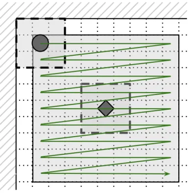
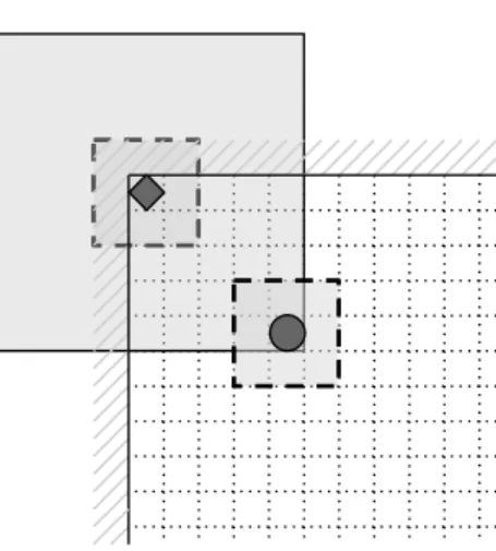
Non-Local Means(NL-means) algorithm at its core operates the same way, but uses a weight function that not only takes into account the intensity values of argument pixels, but also values of pixels in areas surrounding argument pixel, we will refer to these areas as patches — see figure 2.2.
Figure 2.2: A single Non-Local Means iteration evaluating similarity between the denoised pixel (marked with diamond) and pixels of the search window. The areas around the pixels are “patches” and the large area around the central pixel is the “search window”
A patchBf(p) is a square neighborhood centered atpand being of size 2f+1×2f+1
pixels. The level of similarity between pixelspandq, as defined by NL-means method, depends on the squared Euclidean distance between vectors v(B(p)) and v(B(q)), wherev(B(x)) is a vector comprised of intensity values of pixels within patch centered at x:
d2 =d2(B(p, f), B(q, f)).
This method is efficient enough and has the useful property of assigning more weight to patches of similar geometrical configuration, since the order of pixels in patches is taken into account. In its final form, the weighting metric used in NL-means is a decreasing function of Euclidean distance:
w(p, q) = exp −max(0, d
2−2σ2)
h2
!
,
where σ denotes the estimated standard deviation of the noise and h is the filtering parameter.
Some related works state that there are better weigh estimation techniques such as described in [DDT11, Goo76]. Although Euclidean distance is not the best estimate of patches similarity, we deem it sufficient for scalability considerations of the parallel version of the described algorithm.
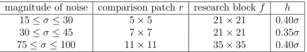
The size of the patch and research window depend on the value of σ. When σ
increases a larger patch is needed to make patch comparison effective. At the same time, the research window must be enlarged as well to increase the noise removal capacity of the algorithm by finding more similar pixels. Authors of original NL-means implementation list values for r, f and hthat produce sufficiently good results for a given level of noise (σ) [BCM05]. Values suggested for certain intervals of σ in case of a monochrome image are provided in table 2.1.
magnitude of noise comparison patch r research block f h
15≤σ ≤30 5×5 21×21 0.40σ
30≤σ ≤45 7×7 21×21 0.35σ
75≤σ≤100 11×11 35×35 0.40σ
Table 2.1: filtering parameters for various levels of noise
For an example of Non-Local Means denoising see figure 2.3.
NL-means parallel processing
As noted above, and can also be inferred from the description of the algorithm, the NL-means method is computation-intensive, but its operational area is limited to relatively small part of the image. Typical image would have at least 100 times bigger linear dimensions than those of the “research” block required to process any specific pixel. This allows to apply split-and-merge strategy. By trying out different sizes of clusters of such units we try to estimate how well can this scheme be scaled and to what extent it can be treated as an embarrassingly parallel computation.
Figure 2.3: Example of image denoising: (a) original image, (b) same image with intentionally added Gaussian noise, (c) Gaussian blur filter applied to the noisy image and (d) NL-means filter applied to the noisy image withσ = 18
2.3
NL-means algorithm implementation in Java
with MapReduce
In current work we apply the NL-means algorithm to reduce noise from images acquired by SAR, and we will put this algorithm to work in a distributed computing environment through instruments of the Hadoop application platform. Since the Hadoop system runs natively on a Java platform, we will use Java language to implement the NL-means algorithm.
The algorithm itself is mostly a straightforward implementation of the iterative filtering procedure described earlier, but has some adjustments that are inherently required by the fact that we are processing not the whole image, but a certain part of that image, as we are running the whole process in a distributed fashion.
NL-means and boundary conditions
Let us examine what behavior the said algorithm must imply when working within boundary regions (pixels adjacent to the edge of image). More specifically consider limitations that arise when following conditions are met:
(a) The patch around reference pixel 2 intersects image border. This occurs
when the reference pixel is close to the edge of image, so that a patch of prescribed size and form cannot be used. We solve this by modifying the shape of a patch used for denoising the pixel at hand (fig. 2.4). This reflects the fact that there is less information on neighborhood of the reference pixel and therefore the weighting estimate is less accurate as well, because smaller vectors will be used to calculate Euclidean distance.
Figure 2.4: Example of boundary condition (a) and its resolution. Diamond marks the reference pixel.
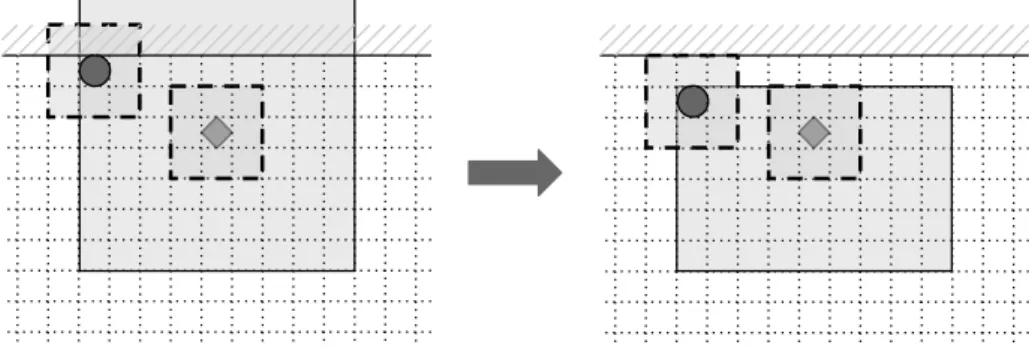
(b) The patch around any pixel that belongs to research window intersects image border. This occurs when the research window intersects with or is
cent to the edge of the image (fig. 2.5).This case can be worked around by reducing the research window from the side that is adjacent to image edge. Moreover, the size of patch must be taken in consideration and there must be left a gap the size of patch radius that would allow to use a patch or prescribed size. Note that this leads to a smaller number of patches to be compared against the current pixel.
Figure 2.5: Example of boundary condition (b) and its resolution. Diamond marks the reference pixel.
(c) Both conditions (a) and (b) are met. At points where both conditions hold (fig. 2.6), we can effectively apply both solutions described in (a) and (b).
Figure 2.6: Example of boundary condition (c) and its resolution. Diamond marks the reference pixel.
One way or another, any of above-mentioned conditions result in less accurate noise correction, and hence must be avoided wherever possible. More precisely, the split-merge approach used to process the image by separate workers must not introduce any new points of boundary conditions in addition to these existing in the original image. That way the distributed algorithm is assured to produce exactly the same result as a single-pass processing. This accuracy was confirmed on results of tests made during current research.
Splitting image for distributed processing
For the sake of simpler presentation of techniques used in current work we will adhere to a simplified method of splitting image matrix into chunks, namely we will divide the matrix into horizontally spreading “stripes”, meaning that the width (number of columns of pixels) of each submatrix is equal to the width of the full image matrix.
If the original image is split into chunks that are simply located one beside another (containing no shared pixels), then each chunk will contain additional points that meet border condition and consequently will suffer from loss of accuracy. In order to overcome this, each chunk needs to be constructed in such a way that it overlaps with neighbouring chunks — this way some additional pixels located “over the edge” are provided along with chunk data and can be used by the NL-means algorithm when computing pixels near junctions of stripes — see figure 2.7.
s1
s2
(a) (b)
Figure 2.7: Example of picture division into two parts with (b) and without (a) over-laps. Darker area indicates the set of pixels where a border condition is met. The part of image marked with “s1”/“s2” is available while processing top/bottom half of the
image.
Also, when splitting the image using overlaps, we store the size of top and bottom overlaps in the input file as well. This way the unprocessed area of the chunk will be known beforehand, so the denoising process will be able to use pixels located in overlapping area, but also will be able to bypass pixels in the overlapping area, which are denoised by another worker. With regard to the noise reduction algorithm this means that there is no computational overhead added if compared to processing of a single monolithic image.
However, overlappings bring storage overhead, amount of which depends on the number of splits and the size of overlapping area. For instance, given an image of size 8064×8064, by dividing it into 48 splits with extra 22 pixels on each side the result will contain 16.18×10⁶ additional pixels, that comprises 26% of the original image
Joining the parts
The resulting image is composed by taking one by one splits produced in the map-ping phase, removing the overlap areas and concatenating into one image file. The concatenation takes place outside of the map-reduce cycle, because the reduce task generally should not output larger amount of data than there was in the input, which would be the case of joining the parts of image together. The Reduce step is bypassed by committing to the Hadoop a parameter indicating that number of Reduce workers must be zero throughout the job.
Once the MapReduce is successfully finished, the program will fetch resulting chunks from the HDSF and run the concatenation writing the output to local disk. This can be done on any computer having access to the HDFS. As as an easy choice it might be convenient to run it on the master node of a cluster to be “closer” to the file storage.
Chapter 3
Validations
3.1
End-to-end process overview
To validate the proposed solution we implemented the NL-means algorithm in Hadoop MapReduce and performed benchmarking experiments on test image. To sum up, the implementation of image filtering that we provide consists of following steps:
I. Prepare input for Hadoop job.
1) Split the input into chunks including additional area on the edges (overlapping zones). Output is written to local files, one per chunk. File format is defined by the custom implementation of Writable. This step is I/O intensive, files are read and written locally. Master node of a cluster can be used to run this operation, because typically it does not operate as the Map/Reduce worker and thus has somewhat less specific purpose. For this work we use a custom Java implementation that can split images (BMP or PNG format).
2) Copy split files to HDFS. In context of current implementation this is made a separate step to ease testing of different input parameters (sigma mainly) or algorithm implementations. This can also be useful when the desired chain of filters to be applied is not known in advance. Alternatively this operation can be carried out immediately in the splitting step, this way no additional files would need to be written locally.
II. Schedule the MapReduce job. Map tasks are executed on worker nodes, the noise reduction algorithm is invoked in parallel. Reduce tasks are omitted, output is written to HDFS as serialized Writable objects. For current work we use a blocking wait call after scheduling the job, so the next step is started after the Hadoop have reported back on job completion.
III. Join result chunks. Parts are fetched from distributed storage, the result written locally as an image file. Current implementation is storing all fetched chunks in memory to create the output file.
3.2
Testing environment and dataset
For measuring execution time we used a cluster of machines hosted on Amazon Elastic Compute Cloud. The cluster is composed of nine virtual machine instances, all having same parameters: two 64-bit virtual CPUs based on Intel Xeon 2.3GHz processors, 1.7 GB of main memory. One of nine machines is chosen to be a master node and acts as a JobTracker as well as an HDFS NameNode, while each of other machines act as TaskTrackers and DataNodes to execute tasks and store files. The size of cluster will vary from 1+1 to 1+8 nodes to rate scalability of the process.
Since the standard setup of Hadoop TaskTrackers allocates as many executor slots as there are processors available to the system, in case of N worker nodes there will be up to N ×2 parallel executions of Map task at hand. That is, the number of task executors will vary from 2 to 16 between tests.
As an input dataset the image of size 8064×8064 (roughly 65·106) pixels was
used. Each pixel is represented by an 8-bit single-channel (monochrome) value. The image is divided into 48 chunks with overlap area size of 22 pixels. For parameter σ a value of 40 was used, so that the search window size is 35 and the patch size is 7.
3.2.1
Test results for sequential parts
Splitting and merging steps (I, III) were executed on a master node as parts of end-to-end process and their times were measured separately.
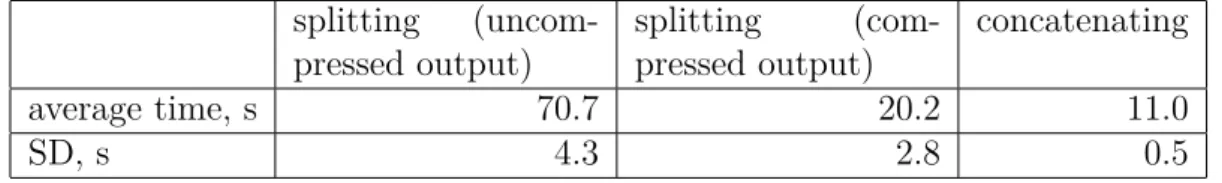
It may be worth mentioning a few things about compression of files holding splits data. By default Hadoop uses Zlib compression to write records into files. During input image splitting (step I) this brings notable performance overhead (see table 3.1), but also results in smaller size of chunk files. In our case compressed split files were about 3 times smaller, which is rather expected, considering that for the sake of simplicity the data structure and the corresponding Writable implementation we used were not intended to have any storage optimization.
splitting (uncom-pressed output) splitting (com-pressed output) concatenating average time, s 70.7 20.2 11.0 SD, s 4.3 2.8 0.5
Table 3.1: Mean time and standard deviation (SD) of steps I and III
By default the Hadoop framework stores output of Map tasks in an uncompressed form, so the results collecting step in our tests did not perform any additional decom-pression.
3.2.2
Parallel execution test results
Here we present run times of Hadoop job itself, i.e. step II in the flow described above. At least five tests were performed for each number of worker nodes: 1, 2, 4, 6 and 8, where number of task executors were 2, 4, 8, 12 and 16, respectively.
To rate how scalable the process is we measured time to see how throughput grows with respect to the increasing number of nodes. A perfect scalability presumes that the throughput changes in proportion to the change in number of processing units.
The average time of execution on N task executors is multiplied by N to get a factor of “serial” run time (as if run sequentially on single processor), that can be compared among different cluster sizes to see how parallelization affects performance.
Speedup is calculated with
S(p) = T1
Tp
,
where p is the number of executors and Tp is execution time withp processors.
Simi-larly, efficiency is
T1
Tp·p
.
For both metrics the run time for one processor was simulated as half of the time for two processors: T1 ≈ T22 (efficiency and speedup shown here are relative and do not
reflect the difference between the actual sequential execution and the parallel one).
number of executors (p) 2 4 8 12 16
Hadoop job time, s 9,229 4,639 2,359 1,569 1,187 “serial” time, s 18,458 18,556 18,868 18,828 18,992 parallel speedup 2.00 3.98 7.83 11.76 15.55 scaling efficiency 1.000 0.995 0.978 0.980 0.972
Table 3.2: Hadoop job averages.
Here we also would like to note that Hadoop jobs operating with compressed files most times showed to be no more performant compared to jobs that got their input uncompressed. For this reason the average times include both variants of execution.
Although mean estimates of speedup and efficiency presented in table 3.2 are rel-ative (based on the run time T2), they show that in our scenario the part that is run
in parallel has very good scaling capability.
3.2.3
Comparison to non-parallel execution
The same algorithm written in Java was applied to the same image as a standalone process traversing the whole image successively. Average time for standalone execu-tions was 16676 seconds (4 hours, 37 minutes and 56 seconds), standard deviation = 21.5 s.
For calculating average end-to-end time in case of Hadoop processing we used the sum of averages in each step (I+II+III). For step I we used the time of a worse scenario, i.e. splitting that produces compressed record files (see table3.1). For step II we used Hadoop job time (see table3.2). The time before, between and after the three describes steps (e.g. process start-up) was always around 3–5 seconds, we considered its amount negligible and chose to ignore it. E.g., end-to-end Hadoop time in case of four executors was calculated as follows:
We compared Hadoop and standalone execution times to evaluate parallel speedup and efficiency using formulas mentioned above, based upon T1 = 16,676 s, see table
3.3.
number of executors (p) 2 4 8 12 16
I+II+III time, s 9311 4721 2440 1651 1269 parallel speedup 1.791 3.533 6.834 10.102 13.144 scaling efficiency 0.896 0.883 0.854 0.842 0.822
Table 3.3: End-to-end execution averages.
Consider the chart showing dependency of speedup from the number of executors (figure 3.1) as an overview of collected metrics.
Figure 3.1: Speedup increase with number of executors: ideal (theoretical limit of parallel speedup) and empirically acquired magnitudes of speedup — “relative” as in table 3.2 and “actual” as in table 3.3.
Comparison to larger input dataset
Same cluster of 1+8 nodes (16 processors) was also used on an image 4 times as big — 16128×16128, roughly 260×106, pixels. The image was split into 96 parts, which produces the same relative amout of overlappings area as in case of the smaller image, i.e. ≈ 26%. The average execution time parallel step (II) was 4289 s, that is 3.61 times slower than time of smaller image on same cluster.
This gives some insight on the efficiency metrics provided above, because it can be seen that in case of larger image the parallel speedup was improved to some extent (otherwise the relation of run time for larger image to the run time of smaller image would be ≥4).
3.3
Amdahl’s prediction
Let us say a few words about the expected theoretical speedup in a cluster with a large number of executors. A classical estimate for a speedup of an algorithm executed in parallel is given by Amdahl’s law (see [Wik14a]).
Amdahl’s law.
If we can measure the partα of the algorithm that can only be executed sequen-tially (while the rest can be parallelized ideally), then the speedupSnobtained by
using n parallel executors can be estimated from above by
Sn∗ = 1
α+ 1−α n
.
In our case, it is reasonable to calculate α as the fraction of processor time spent on steps I and III compared to time spent on steps I, II and III for some number n
of processors. Since the time spent on step II increases with n, the largest (and the worst) α would be for n = 2. So the data from tables 3.1 and 3.2 give us
α= 70.7 + 11.0
70.7 + 18,458 + 11.0 ≈0.0044.
Hence, the theoretical speedup limit for, e.g., n= 256 is S256∗ ≈120.6.
However, we should also account for the non-ideal scaling efficiency of our par-allelization (see table 3.2). In order to estimate this efficiency at n = 256, let us extrapolate the relative speedup linearly (which figure 3.1 suggests is a sane thing to do). This would give us the relative speedup of 247.5× at n = 256 and the corre-sponding relative scaling efficiency ϕn ≈ 0.967. Thus a more precise estimate for the
speedup is Sn/ 1 α+ϕ1−α n·n . In particular, S256/118.7.
3.4
Conclusions
The present work approaches the problem of image filtering by way of parallel comput-ing with the use of MapReduce model on the Hadoop framework. The chosen platform is well-suited for running the NL-means algorithm in a cluster of nodes that store and process data in a distributed fashion.
The level of scalability achieved during experiments shows a good potential of dis-tributed processing in the context of noise reduction and similar image refinement tasks. The comparison of execution times between a Hadoop job and a single pro-cess gives reasons to infer that increased throughput comes at cost of an overhead, which includes latency of Map/Reduce tasks invocation and data interchange. Re-lated research [SJV12] also had identified job execution latency as one of the reasons of incurred overhead.
Nevertheless overhead is not very significant and overall level of scalability allows to increase performance at a reasonable cost.
We would like to note that results of experiments performed on larger amount of data allow us to imply that even higer rates of scaling efficiency are reachable (e.g. for larger sizes of inputs splits). This relation requires a more thorough investigation, though.
From the implementation point of view we would like to note that adapting the solution to the Hadoop framework was fairly easy, at the same time providing con-venience and useful properties of automated distributed computing. We find this trade-off quite beneficial.
Bibliography
[ASF14] Apache Software Foundation. Powered by hadoop — Hadoop Wiki, May 2014. [Online; accessed 14-May-2014]. URL: http://wiki.apache.org/
hadoop/PoweredBy.
[BCM05] A. Buades, B. Coll, and J. M Morel. A non-local algorithm for image denoising. InComputer Vision and Pattern Recognition, 2005. CVPR 2005. IEEE Computer Society Conference on, volume 2, pages 60–65 vol. 2, June 2005.
[BCM11] Antoni Buades, Bartomeu Coll, and Jean-Michel Morel. Non-Local Means Denoising. Image Processing On Line, 2011, 2011. http://dx.doi.org/
10.5201/ipol.2011.bcm_nlm.
[DDT11] C-A Deledalle, L. Denis, and F. Tupin. Nl-insar: Nonlocal interfero-gram estimation. Geoscience and Remote Sensing, IEEE Transactions on, 49(4):1441–1452, April 2011. doi:10.1109/TGRS.2010.2076376.
[DG08] Jeffrey Dean and Sanjay Ghemawat. Mapreduce: Simplified data processing on large clusters. Commun. ACM, 51(1):107–113, January 2008.
[DTD10] C-A Deledalle, F. Tupin, and L. Denis. Polarimetric sar estimation based on non-local means. InGeoscience and Remote Sensing Symposium (IGARSS), 2010 IEEE International, pages 2515–2518, July 2010.
[Goo76] J. W. Goodman. Some fundamental properties of speckle. Journal of the Optical Society of America (1917-1983), 66:1145–1150, November 1976.
[Key92] W. Keydel. Basic principles of SAR. AGARD, Fundamentals and Special Problems of Synthetic Aperture Radar (SAR) 13 p (SEE N93-13049 03-32), August 1992.
[SJV12] Satish Narayana Srirama, Pelle Jakovits, and Eero Vainikko. Adapting sci-entific computing problems to clouds using mapreduce. Future Generation Computer Systems, 28(1):184–192, 2012.
[Wik14a] Wikipedia. Amdahl’s law — Wikipedia, The Free Encyclopedia, May 2014. [Online; accessed 14-May-2014]. URL: https://en.wikipedia.org/wiki/
Amdahl%27s_law.
[Wik14b] Wikipedia. Apache Hadoop — Wikipedia, The Free Encyclopedia, May 2014. [Online; accessed 14-May-2014]. URL: https://en.wikipedia.org/
[Wik14c] Wikipedia. Fork–join model — Wikipedia, The Free Encyclopedia, May 2014. [Online; accessed 14-May-2014]. URL: https://en.wikipedia.org/
wiki/Fork%E2%80%93join_model.
[Wik14d] Wikipedia. Synthetic aperture radar — Wikipedia, The Free Encyclopedia, May 2014. [Online; accessed 14-May-2014]. URL:https://en.wikipedia.
Non-exclusive licence to reproduce thesis and make thesis public
I, Jevgeni Võssotski (date of birth: 08.03.1983),
1. herewith grant the University of Tartu a free permit (non-exclusive licence) to:
1.1 reproduce, for the purpose of preservation and making available to the public, including for addition to the DSpace digital archives until expiry of the term of validity of the copyright, and
2.2 make available to the public via the web environment of the University of Tartu, including via the DSpace digital archives until expiry of the term of validity of the copyright,
of my thesis
SAR Image Denoising Using Non-Local Means on MapReduce, supervised by Pelle Jakovits,
2. I am aware of the fact that the author retains these rights.
3. I certify that granting the non-exclusive licence does not infringe the intellectual property rights or rights arising from the Personal Data Protection Act.
![Figure 1.1: Hadoop cluster setup example, source: Wikipedia[Wik14b]](https://thumb-us.123doks.com/thumbv2/123dok_us/9726434.2854162/9.892.155.727.569.1020/figure-hadoop-cluster-setup-example-source-wikipedia-wik.webp)