Using an Instrumental Variable to Test for Unmeasured Confounding

University of Pennsylvania

ScholarlyCommons

Statistics Papers Wharton Faculty Research

9-10-2014

Using an Instrumental Variable to Test for

Unmeasured Confounding

Jing Cheng

Scott A. Lorch

Dylan S. Small

Zijian Guo

Follow this and additional works at:http://repository.upenn.edu/statistics_papers Part of theStatistics and Probability Commons

Recommended Citation

Cheng, J., Lorch, S. A., Small, D. S., & Guo, Z. (2014). Using an Instrumental Variable to Test for Unmeasured Confounding.Statistics in Medicine, 33(20), 3528-3546.http://dx.doi.org/10.1002/sim.6227

Using an Instrumental Variable to Test for Unmeasured Confounding

Abstract

An important concern in an observational study is whether or not there is unmeasured confounding, that is, unmeasured ways in which the treatment and control groups differ before treatment, which affect the

outcome. We develop a test of whether there is unmeasured confounding when an instrumental variable (IV) is available. An IV is a variable that is independent of the unmeasured confounding and encourages a subject to take one treatment level versus another, while having no effect on the outcome beyond its encouragement of a certain treatment level. We show what types of unmeasured confounding can be tested for with an IV and develop a test for this type of unmeasured confounding that has correct type I error rate. We show that the widely used Durbin–Wu–Hausman test can have inflated type I error rates when there is treatment effect heterogeneity. Additionally, we show that our test provides more insight into the nature of the unmeasured confounding than the Durbin–Wu–Hausman test. We apply our test to an observational study of the effect of a premature infant being delivered in a high-level neonatal intensive care unit (one with mechanical assisted ventilation and high volume) versus a lower level unit, using the excess travel time a mother lives from the nearest high-level unit to the nearest lower-level unit as an IV.

Keywords

instrumental variables, observational study, confounding, comparative effectiveness Disciplines

Using an Instrumental Variable to Test for Unmeasured

Confounding

Jing Cheng

University of California, San Francisco (UCSF)

Scott A. Lorch

University of Pennsylvania

Dylan S. Small

University of Pennsylvania

Abstract: An important concern in an observational study is whether or not there is unmeasured confounding, i.e., unmeasured ways in which the treatment and control groups differ before treatment that affect the outcome. We develop a test of whether there is unmeasured confounding when an instrumental variable (IV) is available. An IV is a variable that is independent of the unmeasured confounding and encourages a subject to take one treatment level vs. another, while having no effect on the outcome beyond its encouragement of a certain treatment level. We show what types of unmeasured confounding can be tested with an IV and develop a test for this type of unmeasured confounding that has correct type I error rate. We show that the widely used Durbin-Wu-Hausman (DWH) test can have inflated type I error rates when there is treatment effect heterogeneity. Additionally, we show that our test provides more insight into the nature of the unmeasured confounding than the DWH test. We apply our test to an observational study of the effect of a premature infant being delivered in a high-level neonatal intensive care unit (one with mechanical assisted ventilation and high volume) vs. a lower level unit, using the differential distance a mother

∗_{Corresponding author. Division of Oral Epidemiology & Dental Public Health, UCSF School of}

lives from the nearest high-level unit to the nearest lower-level unit as an IV.

1

Introduction

An observational study is a comparison of treatment groups in which “the objective is to elucidate cause-and-effect relationships [... in which it] is not feasible to use controlled experimentation in the sense of being [able]... to assign subjects at random to different procedures” (Cochran, 1965). A central concern in an observational study is confounding, meaning that the treatment groups may differ before treatment in ways that affect the outcome. If the ways in which the treatment groups differ are measured, these differences can be adjusted for, e.g., by matching, stratification or regression (Rosenbaum, 2001). However, there is often concern that there unmeasured ways in which the treatment groups differ that affect the outcome, meaning that there is unmeasured confounding. Even when there is unmeasured confounding, it is possible to obtain a consistent estimate of the causal effect of treatment for a certain subpopulation (the compliers) if an instrumental variable (IV) can be found. An IV is a variable that is independent of the unmeasured confounding and encourages, but does not force a subject to take one treatment level vs. another, while having no effect on the outcome beyond its encouragement of a certain treatment level. For discussions of IVs, see Angrist, Imbens and Rubin (1996), Abadie (2002), Hern´an and Robins (2006), Tan (2006), Brookhart and Schneeweiss (2007), Cheng, Qin and Zhang (2009) and Tan (2010). In this paper, we develop a method for using an IV to test whether there is unmeasured confounding. Detecting whether there is unmeasured confounding is valuable in many studies because if unmeasured confounding is found in a given study, it suggests that for studying related questions, researchers should either try to measure more confounders or seek to find IVs.

The existing and widely used test for whether there is unmeasured confounding using an IV is the Durbin-Wu-Hausman endogeneity test, hereafter called the DWH test,

indepen-dently proposed by Durbin (1954), Wu (1973) and Hausman (1978). The DWH test compares an estimate of the average treatment effect under the assumption that there is no unmea-sured confounding to an estimate of the average treatment effect using an IV that allows for unmeasured confounding. The IV estimate of the average treatment effect is assumed to be consistent so that a significant difference between it and the estimate that assumes no unmea-sured confounding is taken as evidence of unmeaunmea-sured confounding. The two estimates of the average treatment effect in the DWH test assume that the treatment effect is homogeneous, meaning that it is not associated with measured or unmeasured confounders; see Wooldridge (2003), Hern´an and Robins (2006), Basu et al. (2007), Brookhart and Schneeweiss (2007) and Tan (2010) for discussion of homogeneity assumptions. Brookhart, Rassen and Schneeweiss (2010) noted that if the DWH test rejects, one cannot be sure whether it is because of unmeasured confounding or treatment effect heterogeneity.

In this paper, we discuss what types of unmeasured confounding can be tested for and provide a test with correct type I error rate for the testable types of unmeasured confounding. In addition to having the advantage over the DWH test of having correct type I error rate when there is treatment effect heterogeneity, our testing approach also provides more insight into the nature of the unmeasured confounding by providing separate tests for two different types of unmeasured confounding. In the DWH test, these two types of unmeasured confounding are lumped together.

The motivating application for our work is an observational study of neonatal care that seeks to estimate the effect on mortality of a premature infant being delivered in a high-level neonatal intensive care unit (NICU) vs. a lower-level NICU. A high-level NICU is defined as NICU that has the capacity for sustained mechanical assisted ventilation and delivers at least 50 premature infants per year. Estimating the effect of being delivered at a high-level NICU is important for determining the value of a policy of regionalization of perinatal care that aims for premature infants to be mostly delivered in high-level NICUs. (Lorch, Myers and Carr, 2010). Regionalization of perinatal care was developed in the 1970s along with

the expansion of neonatal technologies, but by the 1990s, regionalization began to weaken in many areas of the United States (Howell et al., 2002). The difficulty in studying the causal effect of a premature infant being delivered in a high-level vs. a lower-level NICU is that the infants who are at most risk of death are most likely to be delivered at a high level NICU. In our data from Pennsylvania (described in Section 6), the unadjusted death rate in high-level NICUs is higher than in low-level NICUs, 2.3% vs. 1.2%. Our data contains a number of potential confounders, including birth weight, gestational age, month prenatal care started, mother’s comorbid conditions, mother’s socioeconomic status and mother’s insurance. After adjustment for these measured confounders by propensity score matching, the death rate is 0.5% lower in high-level NICUs with the difference being not significant at the .05 level (Lorch et al., 2011). However, we are concerned about unmeasured potential confounders, such as the severity of a mother’s comorbid condition or an infant’s antenatal condition, lab results, fetal heart tracing results, the compliance of the mother to medical treatment and the physician’s history with that mother. These variables are known to the physicians who assess a mother’s probability of delivering a high-risk infant. Based on this probability, the physicians then play a role in deciding where the mother should live. To attempt to deal with the problem of potential unmeasured confounding, we have collected data on a proposed IV, the excess travel time that a mother lives from the nearest high-level NICU compared to the nearest lower-level NICU; specifically, the IV is whether or not the mother’s excess travel time is less than or equal to 10 minutes. Excess travel time to a hospital delivering specialty care has been used as an IV in other medical settings, such as studies of the effect of cardiac catheterization on survival in patients who suffered an acute myocardial infarction (McClellan et al., 1994) In obstetric care, prior work suggests that women tend to deliver at the closest hospital with obstetric care so that we expect that excess travel time will have a strong effect on where the infant is delivered (Phibbs, 1993). Our goal in this paper is to use the putative IV excess travel time to test whether there is unmeasured confounding in the study of the effect of high-level vs. lower-level NICUs. If unmeasured confounding is found,

it suggests that previous studies of the effect of high-level vs. lower-level NICUs provide biased estimates and that future studies of this and related medical questions should seek to measure more confounders and/or find and measure IVs.

The rest of the paper is organized as follows. In Section 2, we set up the causal framework and introduce notation and assumptions. In Section 3, we discuss what type of unmeasured confounding can be tested for when there are heterogeneous treatment effects. In Section 4, we discuss the DWH test and how it performs when there are heterogeneous treatment effects. In Section 5, we develop our method for testing unmeasured confounding. In Section 6, we apply our test to the study of the effect of high-level vs. lower-level NICUs. Finally, we provide conclusions and discussion in Section 7.

2

The Framework

2.1

Notation

The IVZ and the treatmentAare assumed to each be binary, where level 0 of the treatment is considered the “control” (lower-level NICU in our application) and level 1 is considered to be the “treatment” (high-level NICU in our application). We letZdenote theN-dimensional vector of IV values for allN subjects, with individual elementsZi =z ∈ {0,1}for subject i;

level 1 of the IV is assumed to encourage receiving the treatment compared to level 0. LetAz

be the N-dimensional vector of potential treatment under IV assignment z, with individual element Az_i =a∈ {0,1} according to whether subjecti would take the control or treatment under z. We let Yz,a _{be the vector of potential responses that would be observed under IV}

levels z and treatment levelsa, with individual element Y_ir,a for subject i. {Y_ir,a} and {Ar i}

are “potential” responses and treatments in the sense that we can observe only one value in each set. We let Yi and Ai be the corresponding observed outcome and treatment variables

for subjecti. We let Xi denote the measured confounders for subjecti. We assume that Xi

2.2

Assumptions

We make the same assumptions as Angrist et al. (1996) within strata of the measured confounders X.

Assumption 1: Stable unit treatment value assumption (SUTVA) (Rubin, 1986): (a) If z = z′, then

Az i = Az ′ i . (b) If z = z ′ and a = a′, then Y_iz,a = Yz ′ ,a′

i . This assumption allows us to

write Y_iz,a and Az_i as Y_iz,a and Az_i, respectively, for subject i.

Assumption 2: IV is independent of unmeasured confounding: Conditional on X, the IV Z is indepen-dent of the vector of potential responses and treatments (Y0,0_{, Y}0,1_{, Y}1,0_{, Y}1,1_{, A}0_{, A}1_)for

a randomly chosen subject.

Assumption 3: Exclusion restriction: For subject i, Y_iz,a = Y_iz′,a for all z, z′ and a, i.e., the IV level affects outcomes only through its effect on treatment level. This assumption allows us to define Ya i ≡Y 0,a i =Y 1,a i for a= 0,1.

Assumption 4: Nonzero average causal effect of Z on A: E(A1−A0|X)̸= 0.

Assumption 5: Monotonicity: P(A1 _≥A0_{) = 1. This assumption says that there is no one who would}

always do the opposite of what the IV encourages, i.e., no one who would not take the treatment if encouraged to do so by the IV level but would take the treatment if not encouraged by the IV level.

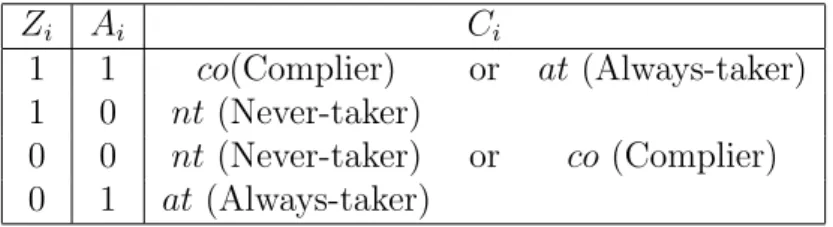
Table 1: The relation of observed groups and latent compliance classes under the monotonic-ity assumption Zi Ai Ci 1 1 co(Complier) or at (Always-taker) 1 0 nt(Never-taker) 0 0 nt(Never-taker) or co (Complier) 0 1 at (Always-taker)

2.3

Compliance Class

Based on a subject’s joint values of potential treatment (A0

i, A1i), a subject can be classified

into one of four latent compliance classes (Angrist et al., 1996):

Ci =                  nt(never-taker) if (A0 i, A1i) = (0,0) co (complier) if (A0_i, A1_i) = (0,1) at(always-taker) if (A0_i, A1_i) = (1,1) de (defier) if (A0 i, A1i) = (1,0)

Under the monotonicity assumption, there are no defiers. We can observe only one of A0_i and A1_i, so a subject’s compliance class is not observed directly but it can be par-tially identified based on IV level and observed treatment as shown in Table 1. Based on Table 1, the following quantities are identified based on the observable data: P(C =

at) = P(A = 1|Z = 0), P(C = nt) = P(A = 0|Z = 1), P(C = co) = 1− P(A = 1|Z = 0)− P(A = 0|Z = 1), E(Y1_{|C = at) = E(Y|Z = 0, A = 1), E(Y}0_{|C = nt) =} E(Y|Z = 1, A = 0), E(Y1|_{C = co) =} E(Y|Z=1,A=1)−[P(C=at)/{P(C=at)+P(C=co)}]E(Y|Z=0,A=1) P(c=co)/{P(C=at)+P(C=co)} and E(Y0|_{C = co) =} E(Y|Z=0,A=0)−[P(C=nt)/{P(C=nt)+P(C=co)}]E(Y|Z=1,A=0) P(c=co)/{P(C=nt)+P(C=co)} . The quantities

3

Type of Unmeasured Confounding that Can Be Tested

For Using an IV

The average treatment effect is E(Y1 − Y0). Rosenbaum and Rubin (1983) and Imbens (2004) discuss how the average treatment effect can be consistently estimated by propensity score methods, matching methods regression methods under the following two assumptions:

0< P(A= 1|X)<1 (1)

(Y1, Y0)⊥⊥A|X. (2) Assumption (1) says that the support of the covariate distributions of the treated and control units is the same; this is called the overlap assumption. Assumption (2) is called the un-confoundedness assumption and holds if there are no unmeasured confounders of treatment assigment (i.e., no unmeasured variables that are associated with both treatment assignment and outcome). When the overlap assumption (1) does not hold, but the unconfoundedness assumption (2) holds, then the average treatment effect on the common support of the co-variate distributions of the treated and controls subjects can be consistently estimated. For consistent estimation of the average treatment effect, the following conditions implied by (2) are sufficient (Heckman, Ichimura and Todd, 1998; Imbens, 2007):

E(Y1|A= 1,X) = E(Y1|A= 0,X), (3)

E(Y0|A= 1,X) = E(Y0|A= 0,X). (4)

We will show that having a valid IV Z allows us to test certain aspects of (3)-(4), but not other aspects.

classes: E(Y1|A= 1) = P(C=at|X) P(C=at|X) +P(Z = 1|X)P(C =co|X)E(Y 1_{|C=at,X) +} P(Z = 1|X)P(C =co|X) P(C=at|X) +P(Z = 1|X)P(C =co|X)E(Y 1_{|C=co,X), (5)} E(Y1|A= 0) = P(C =nt|X) P(C=nt|X) +P(Z = 0|X)P(C=co|X)E(Y 1_| C =nt,X) + P(Z = 0|X)P(C =co|X) P(C=nt|X) +P(Z = 0|X)P(C=co|X)E(Y 1_{|C =co,X). (6)}

Although there are a variety of ways for (5) to equal (6), the way that seems most easily discussed with collaborators as to whether it is plausible and that is most easily generalized to other related studies is for the expected potential outcome under treatment given the measured confounders X to be the same for all three compliance classes:

E(Y1|C =at,X) = E(Y1|C =co,X) = E(Y1|C =nt,X). (7) As discussed in Section 2.3, the IV Z identifies E(Y1_{|C =at,X) and E(Y}1_{|C =co,X) but}

not E(Y1_{|C =nt,X). Thus, we can test the following aspect of (7):}

E(Y1|C =at,X) = E(Y1|C =co,X) for all X. (8) Similarly, a way for (4) to hold is for

E(Y0|C =at,X) = E(Y0|C =co,X) = E(Y0|C =nt,X), (9) and the IV Z enables us to test the following aspect of (9):

E(Y0|C =co,X) = E(Y0|C =nt,X) for all X. (10) To summarize, a valid IV Z enables us to test the aspects (8) and (10) of (7) and (9)

respectively, where (7) and (9) holding together ensure that the no unmeasured confounders assumption (2) holds.

We now discuss what information is learned from the test of (8) and (10). Suppose one of tests rejects, e.g., suppose there is evidence that E(Y1|_{C = at,X) > E(Y}1|_{C = co,X).}

Then, in the NICU study (where Y is mortality), conditional on measured confounders X, among the always takers and compliers, infants who are more likely to be delivered at a high level NICU (always takers) are in worse underlying condition than infants who are less likely to be delivered at a high level NICU (compliers). This indicates that there are unmeasured confounders that are associated with both (i) selection of whether to go to a high level NICU and (ii) mortality. It is still possible that the unconfoundedness assumption (2) assumption holds through some cancellation of the effects of these unmeasured confounders with other unmeasured confounders, but it seems unlikely. Now suppose that the (8) and (10) are true. This does not necessarily imply that unconfoundedness (2) holds, but it does imply that (2) holds under the following additional assumption that the average treatment effect is the same for the different compliance classes conditional on the measured confounders X:

E(Y1−Y0|C=at,X) =E(Y1−Y0|C =co,X) =E(Y1−Y0|C =nt,X).

4

DWH Test

The DWH test statistic TDW H is the following. Let ˆβOLS denote the ordinary least squares

(OLS) estimates of the regression ofY onAand Xand let ˆβ_2SLS denote the two stage least squares (2SLS) estimates of the effects ofA andX onY, namely ˆβ_2SLS is computed by first regressingAonZ,Xby least squares and finding the predicted value ˆAand then regressingY

on ˆA,X by least squares. The DWH test statistic is an assessment of the difference between the OLS and 2SLS estimates,

TDW H = ( ˆβOLS −βˆ2SLS) T

where (Cov{βˆ_2SLS} −Cov{βˆ_OLS})+ _{is the Moore-Penrose pseudo-inverse of (Cov{βˆ}

2SLS} −

Cov{βˆ_OLS})+_{. The covariances in (11) are the covariances that come for the normal linear}

regression model or normal simultaneous equations model that make the homoskedasticity assumption that V ar(Y0|_{X) is equal to V ar(Y}1|_{X) and the same for all X, Under the null}

hypothesis that the aspects (8) and (10) of unconfoundendess hold in addition to the average treatment effect for compliers being homogeneous inX(i.e.,E(Y1−Y0|C =co,Xis the same for all X), E(Y0|X) being linear in X and a homoskedasticity assumption that V ar(Y0|X) is equal to V ar(Y1|X) and the same for allX, the null distribution of TDW H is chi-squared

with 1 degree of freedom (Durbin, 1954; Wu, 1973; Hausman, 1978).

We now consider the properties of the DWH test when the aspects (8) and (10) hold, but average treatment effects are heterogeneous in X. The DWH test statisticTDW H is the

difference between the ordinary least squares estimate of the treatment effect from a linear regression of Y on A and X (namely, the coefficient on A in this linear regression) and the two stage least squares estimate of the treatment effect that uses the IV Z, namely the coefficient on ˆE(A|X, Z) from a regression of Y on ˆE(A|X, Z) and X, where ˆE(A|X, Z) is obtained from a linear regression ofAonX andZ. Let ˆβOLS and ˆβT SLS denote the ordinary

least squares and two stage least squares treatment effect estimates respectively. Under the null hypothesis that E(Y(_{0)|X) is linear in X and E(Y}(1)_−Y(0)_{|C,X) is the same for all}

C,X, the asymptotic null distribution ofTDW H is a mean zero normal random variable with

variance V ar( ˆβT SLS)−V ar( ˆβOLS), where the variances are under the null hypothesis.

Suppose (8) and (10) hold. We will show that the DWH test may still reject with probability converging to 1 when there are heterogeneous treatment effects. This is because

ˆ

βOLS and ˆβT SLS are converging to different weighted averages of treatment effects. Let

βX = E(Y1 − Y0|C = co,X). Suppose E(Yi|Xi, Ai = 0) is linear in Xi and (8) and

(8) and (10) hold. Then E(Y|A = 1,X) −E(Y|A = 0,X) = βX. Then, we have the

linear projection of A onto B, namely E∗(A|B) = αT_{B,α= arg min} α∗E(A−(α∗)TB, plimβˆOLS = E[(Ai−E∗(Ai|Xi))(Yi−E∗(Yi|Xi))] E[(Ai−E∗(Ai|Xi))2 (12) = E[(Ai−E ∗_(A i|Xi))Yi] E[(Ai−E∗(Ai|Xi))2 (13) = E[(Ai−E ∗_(A i|Xi))E(Yi|Xi, Ai)] E[(Ai−E∗(Ai|Xi))2 (14) = E[(Ai−E ∗_(A i|Xi))(E(Yi|Xi, Ai = 0) +βXAi] E[(Ai−E∗(Ai|Xi))]2 (15) = E[(Ai−E ∗_(A i|Xi))2βX] E[(Ai−E∗(Ai|Xi))2] (16) Thus, the OLS estimator converges to a weighted average of treatment effects at different values of X, where the values of X that get the most weight are those where E[(Ai −

E∗(Ai|Xi))2] is largest. IfE(Ai|Xi) is linear inX, thenE[(Ai−E∗(Ai|Xi))2] is the conditional

variance ofA givenX. We use the fact that any linear function of Xi is independent ofAi−

E∗(Ai|Xi) to derive (13) and (16) and we iterate expectations overXi andAi to derive (14).

IfE(Yi|Xi, Ai = 0) is not linear inXi, thenplimβˆOLS equals (16) plus E[(Ai−E

∗_(Ai|Xi))E(Y0_|X)]

E[(Ai−E∗(Ai|Xi))2] .

Angrist and Krueger (1999) derive similar expressions assuming E(Ai|Xi is linear in Xi.

Similarly,

plimβˆT SLS = E[V ar(E(Ai|Xi, Zi)|Xi)βX]/E[V ar(E(Ai|Xi, Zi)|Xi)]

= E[P(C =co|Xi)2P(Zi = 1|Xi)(1−P(Zi = 1|Xi))βX]

E[P(C =co|Xi)2P(Zi = 1|Xi)(1−P(Zi = 1|Xi))].

Thus, the TSLS estimator converges to a weighted average of treatment effects at different values of X, where the values of X that tend to get the most weight are those for which the proportion of compliers is highest. A value of X at which there are no compliers gets zero weight.

Table 2: Comparison of population, OLS and TSLS weights Condition Population OLS TSLS

Proportion Weight Weight Pregnancy induced hypertension .104 .098 .080

Gestational diabetes .052 .052 .045 Pre-term labor .447 .433 .338

weights for some key variables. Mothers with pregnancy-induced hypertension, gestational diabetes and pre-term labor are less likely to be compliers and hence receive less weight in the instrumental variable two stage least squares analysis.

5

Test Based on IV Propensity Score Subclassification

Estimate

One approach to testing (8)-(10) would be to fit a parametric model for the data as in Hirano, Imbens, Rubin and Zhou (2000) and test (8)-(10) through the parameters of the model. This test might involve a large number of degrees of freedom. To gain more power for the particular contrasts of interest, our approach is to choose a covariate distribution

F(X) that we are interested in and test

EF(Y1|C =at,X) = EF(Y1|C =co,X) (17)

EF(Y0|C =nt,X) =EF(Y0|C =co,X) (18)

Three particular covariate distributions that could be of interest are (1) the distribution of

X over the whole study population; (2) the distribution of X over the compliers; (3) the distribution of X over the compliers and never takers. (1) is of interest for comparing a policy that provides the treatment to everybody to a policy that provides the treatment to nobody; this contrast is not of particular interest for the NICU study because eliminating all high-level NICUs is not a policy that is being considered. (2) is of interest for comparing

a policy that provides the encouraging level of the IV to everybody versus a policy that provides the encouraging level of the IV to nobody; this contrast is of interest for the NICU study because it compares the policy of building enough high level NICUs so that everybody lives close to one to a policy in which there are very few high level NICUs so that everybody lives far from one. (3) is of interest for comparing a policy that provides the treatment to everybody to a policy that provides the not encouraging level of the IV to everybody; this contrast is of interest for the NICU study because it compares the policy of sending all premature infants to high level NICUs to the policy of having few high level NICUs so that most people live far from one.

To estimate the quantities in (17)-(18), we use the approach of subclassification on the IV propensity score of Cheng (2011). This approach is an extension to the IV setting of subclassification on the propensity score for estimating average treatment effects under strongly ignorable treatment assignment (Rosenbaum and Rubin, 1984). The basic idea is that we create subclasses in which the covariate distribution ofXis approximately the same between the Z = 1 and Z = 0 groups, then estimate the quantities in (17)-(18) within the subclass using methods that assume the IV is independent ofXwithin the subclass and then weight the subclass estimates appropriately to obtain overall estimates of (8)-(18).

1. We construct subclasses over which the distribution of the covariatesXin theZ = 1 and

Z = 0 groups are approximately equal. To construct these subclasses, we estimate the IV propensity score, P(Z = 1|X) and then divide the subjects by their IV propensity scores into five subclasses. This borrows Rosenbaum and Rubin (1984)’s approach for estimating average treatment effects under strongly ignorable treatment assignment of subclassifying on the propensity score for treatment assignment, P(A = 1|X). Rosen-baum and Rubin, building on results in Cochran (1968), showed that subclassifying on the propensity score removes approximately 90% of the initial bias in X. Since we are interested in creating subclasses that have an equal distribution between theZ = 1 and

check balance of covariates X in the Z = 1 and Z = 0 groups has been achieved, the diagnostics suggested by Rosenbaum and Rubin (1984) and Stuart (2010) can be used; see our application in Section 6 for an illustration.

2. Within each subclass, the IV Z is approximately independent of X and by Assumption 2 for IVs, Z is independent of any unmeasured confounders. Consequently, within the subclass, Z can be considered to be approximately randomly assigned. For randomly assigned IVs, Cheng (2009) developed maximum likelihood estimates of the quantities

E(Y1_{|C = at), E(Y}1_{|C = co), E(Y}0_{|C = nt), E(Y}0_{|C = co), P(C = at), P(C = co)}

and P(C =at); see Baker (2010) and Cheng (2010) for further discussion.

3. For each subclass, estimatePF(Xin subclass) and weight the subclass estimates by these

probabilities to form the overall estimates. For example, forF being the distribution of

X over the whole study population, we weight the subclasses by the number of subjects in the subclass. For F being the distribution of X over the compliers, we weight the subclasses by ˆP(C=co|subclass)× number of subjects in subclass.

4. We use the bootstrap to obtain confidence intervals forEF(Y1|C=at,X)−EF(Y1|C=

co,X) and EF(Y0|C = nt,X)−EF(Y0|C = co,X), and check if zero is in the

confi-dence intervals; if zero is not in either conficonfi-dence interval, this indicates unmeasured confounding of the type discussed in Section 3. The bootstrap is carried out treating the distribution of the covariatesXand Z as fixed, so that the subclasses and the number of

Z = 1 andZ = 0 within each subclass are the same as the actual data for each bootstrap iteration, and we just resample the (Y, A)|Z = 1 and (Y, A)|Z = 0 within each subclass.

6

Application to Study of High-Level NICUs vs.

Lower-Level NICUs

We obtained birth certificates from all deliveries occurring in Pennsylvania. Each state’s department of health linked these birth certificates to death certificates using name and date of birth, and then de-identified the records. We then matched over 98% of birth certificates to maternal and newborn hospital records using prior methods (references from Scott) Over 80% of the unmatched birth certificate records were missing hospital, suggesting a birth at home or a birthing center. The unmatched records had similar gestational age and racial/ethnic distributions to the matched records. The Institutional Review Boards of The Children’s Hospital of Philadelphia and the department of health in Pennsylvania approved this study. Infants included in this study had a gestational age between 23 and 37 weeks, and a birth weight between 400 to 8000 grams. Birth records were excluded if the birth weight was more than 5 standard deviations from the mean birth weight for the recorded gestational age in the cohort. There are 192,078 infants in the final cohort. The primary outcome for this study is neonatal death, defined as any death during the initial birth hospitalization.

Baiocchi, Small, Lorch and Rosenbaum (2010) discussed a matching approach to esti-mating the complier average causal effect,E(Y1−Y0|C =co), for this study. Here our focus is on using the IV of excess travel time to test for whether there is unmeasured confounding. The IV is Z = 1 if a mother’s excess travel time to the nearest high level NICU compared to the nearest hospital is 10 minutes or less, Z = 0 if her excess travel time is more than 10 minutes. Discussion of IV assumptions for application. Excess travel time is correlated with whether a mother delivers at a high level NICU because a mother typically obtains prenatal care from and would prefer to deliver at a close by facility (Phibbs et al., 1993). Excess travel time is unlikely to have a direct effect on the outcome because presumably, a nearby hospital with a high level NICU only affects the baby if the baby receives care at that hospital. The third assumption, that excess travel time is independent of unmeasured

confounders, is plausible after controlling for measured characteristics that predict where people live (e.g., race and socioeconomic status).

The measured confoundersXinclude birth weight and gestational age; maternal sociode-mographic factors, such as race, age, education, and insurance status; sociodesociode-mographic characteristics of the zip code the mother lives in; maternal comorbid conditions such as gestational diabetes and hypertension; prenatal care and congenital anomalies. We fit a logistic propensity score model P(Z|X = exp(λ

T X)

1+exp(λTX). Following the approach of Crump,

Hotz, Imbens and Mitnik to dealing with limited overlap, we limited our study sample to those infants with propensity scores between 0.1 and 0.9, leaving 165,868 infants. We then divided the infants into five subclasses equally spaced along the range of propensity scores [0.1,0.9], namely [0.10,0.26),[0.26,0.42),[0.42,0.58),[0.58,0.74),[0.74,0.90].

The standardized difference between the infants living near to a high level NICU (Z = 1) and far from a high level NICU (Z = 0) before and after the subclassification are dis-played in Table 3. The standardized difference of a covariate X before subclassification is

¯

Xnear−X¯f ar √

s2

X,near+s2X,f ar/2

(Rosenbaum and Rubin, 1985). This is the difference in means of the co-variate between the near and far group divided by the standard deviation of the coco-variate, where the standard deviation is calculated in a way that gives equal weight to the near and far groups. The standardized difference of a covariate X after subclassification is

∑5 s=1( ¯Xnear,s−X¯f ar,s) √ s2 X,near+s2X,f ar/2 , (19)

where ¯Xnear,s and ¯Xf ar,s are the means of the covariate X for the near and far infants in

subclass s respectively and ws is the proportion of infants in subclass s. The numerator in

(19) is the average difference in means of the covariate X between the near and far groups within a subclass, weighted by the number of infants in the subclass. The denominator in (19) is the standard deviation of the covariate calculated in the same way as for the standardized difference before subclassification. The standardized differences before subclassification in

Table 3 show that near infants had substantially lower birth weight, a later start to prenatal care, were more likely to have non-white mothers, were less likely to have fee for service insurance and more likely to have federal/state insurance and lived in neighborhoods with more poverty. The standardized differences after subclassification are all less than or equal to 0.05 (with most being 0.01 or less) indicating that the subclassification has succeeded in balancing the covariance distribution between the near and far infants within subclasses. Because of space limitations, Table 3 does not show the standardized differences for all of the maternal comborbidities and complications during pregnancy and infant congenital anomalies, but all of these covariates have standardized differences after subclassification of 0.05 or less.

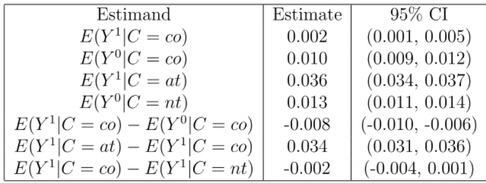
The estimates and confidence intervals for the mean potential outcomes for the compli-ance classes under the covariate distribution of the compliers are shown in Table 4. The fifth line, E(Y1|C =co)−E(Y0|C =co), shows that we estimate that for compliers, attending a high level NICU reduces the death rate by 0.8%, with a 95% confidence interval of a 0.6% to 1.0% reduction. The sixth line, E(Y1|C = at)− E(Y1|C = co), displays the test of unmeasured confounding (8). Always takers appear to have much higher death rates than compliers who attend high level NICUs; the 95% confidence interval for the difference is 3.1% to 3.6%. This is evidence that there is unmeasured confounding. Infants who live far away from high level NICUs but are nevertheless delivered at high level NICUs are in substantially worse health than infants who only deliver at a high level NICU when they live close to one even after controlling for all of the covariates in Table 3. The seventh line, 10, displays the test of unmeasured confounding (10). The death rates of never takers and compliers who deliver at low level NICUs appear to be comparable, and there is not evidence of unmeasured confounding in this dimension. Infants who would always deliver at a low level NICU no matter whether they live near or far from a high level NICU appear to comparable in their health to infants who would deliver at a high level NICU if they lived close to one but a low level NICU if they lived far from a high level NICU.

Table 3: Covariate balance before and after subclassification. The subclasses are the following ranges of propensity scores: [0.10,0.26),[0.26,0.42),[0.42,0.58),[0.58,0.74),[0.74,0.90]; subjects with propensity scores less than 0.1 or greater than 0.9 are not considered. |St-dif|= absolute standardized difference. 1/0 means 1=yes, 0=no. Prenatal care month refers to month in which prenatal care began. Mother’s education scale is a six point scale with high school graduate scored as 3 and college graduate scored as 5. For Zip Code/Census data, fr = fraction of Zip Code. In addition to the results shown, 20 additional maternal complications during pregnancy and ten congenital anomialies also have an absolute standardized difference of 0.05 or less.

Before Subclassification After Subclassification Near Far |St-dif| Near Far |St-dif|

Mean Mean Mean Mean

Covariates Pregnancy and Birth

Birth Weight (grams) 2,552 2,629 0.11 2,613 2,614 0.00 Gestational Age (weeks) 35.02 35.27 0.09 35.20 35.21 0.00 Gestational Diabetes (1/0) 0.05 0.05 0.00 0.05 0.05 0.01 Preg. Induced Hypertension (1/0) 0.11 0.10 0.02 0.10 0.10 0.00

Pre-term labor (1/0) 0.45 0.44 0.03 0.44 0.45 0.00

Prenatal Care (month) 2.43 2.20 0.17 2.24 2.23 0.00

Prenatal Care Missing 0.13 0.07 0.20 0.09 0.09 0.02

Single Birth (1/0) 0.83 0.83 0.00 0.82 0.82 0.05

Parity 2.18 2.04 0.11 2.05 2.05 0.02

Mother

Mother’s Age 28.06 28.04 0.01 28.47 28.47 0.05

Mother’s Education (scale) 3.68 3.70 0.02 3.80 3.80 0.00 Mother’s Education Missing 0.03 0.01 0.14 0.02 0.02 0.00

White (1/0) 0.59 0.85 0.60 0.79 0.79 0.01

Black (1/0) 0.26 0.05 0.65 0.08 0.08 0.02

Asian (1/0) 0.02 0.01 0.08 0.01 0.01 0.00

Other Race (1/0) 0.04 0.02 0.14 0.03 0.03 0.01

Race Missing (1/0) 0.09 0.07 0.05 0.09 0.08 0.01

Mother’s Health Insurance

Fee For Service (1/0) 0.18 0.25 0.18 0.24 0.23 0.01

HMO (1/0) 0.37 0.35 0.05 0.39 0.39 0.04

Federal/State (1/0) 0.33 0.28 0.11 0.26 0.26 0.00

Other (1/0) 0.10 0.09 0.10 0.10 0.10 0.00

Uninsured (1/0) 0.01 0.02 0.04 0.01 0.01 0.00

Mother’s Neighborhood (Zip Code/Census)

Income ($1000) 40 42 0.11 44 44 0.01

Below Poverty (fr) 0.15 0.10 0.19 0.09 0.09 0.00

Home Value ($1000) 92 101 0.02 106 107 0.03

Has High School Degree (fr) 0.79 0.82 0.36 0.82 0.83 0.01 Has College Degree (fr) 0.22 0.20 0.15 0.22 0.22 0.01

Table 4: Inferences for NICU Study Under Covariate Distribution of Compliers Estimand Estimate 95% CI E(Y1|C =co) 0.002 (0.001, 0.005) E(Y0_{|C =co) 0.010 (0.009, 0.012)} E(Y1|_{C =at) 0.036 (0.034, 0.037)} E(Y0|C =nt) 0.013 (0.011, 0.014) E(Y1_{|C =co)−E(Y}0_{|C =co) -0.008 (-0.010, -0.006)} E(Y1|_{C =at)}−_E(Y1|_{C=co) 0.034 (0.031, 0.036)} E(Y1|C =co)−E(Y1|C =nt) -0.002 (-0.004, 0.001)

7

Conclusions and Discussion

We have developed a test of whether there is unmeasured confounding when an instrumental variable (IV) is available. Our test has correct type I error rate unlike the Durbin-Wu-Hausman (DWH) test, which can have inflated type I error rates when there is treatment effect heterogeneity. An important additional advantage of our approach over the DWH test is that it breaks up the test into the two parts (8)-(10), providing more information. For the application, we found that always takers are at much higher risk of death than compliers when both groups are delivered at high level NICUs but there is not a big difference between the never takers and compliers when both groups are delivered at lower-level NICUs.

References

[1] Abadie, A. (2002). Bootstrap tests for distributional treatment effects in instrumental variable models.Journal of the American Statistics Association, 97, 284-292.

[2] Angrist, J.D., Imbens, G.W. and Rubin, D.R. (1996), “Identification of causal effects using instrumental variables (with discussion),”Journal of the American Statistical Asso-ciation, 91, 444-472.

[3] Angrist, J.D. and Krueger, A.B. (1999). Empirical Strategies in Labor Economics, in

[4] Baker, S.G. (2010). Reader reaction: Estimation and inference for the causal effect of Receiving Treatment on a multinomial outcome: an alternative approach.Biometrics, in press.

[5] Basu, A., Heckman, J.J., Navarro-Lozano, S. and Urzua, S. (2007). Use of instrumental variables in the presence of heterogeneity and self-section: an application to treatments of breast cancer patients. Health Economics, 16, 1133-1157.

[6] Brookhart, M.A., Rassen, J.A. and Schneeweiss, S. (2010). Instrumental variable methods in comparative safety and effectiveness research.Pharmacoepidemiology and Drug Safety,

19, 537-554.

[7] Brookhart, M.A. and Schneeweiss, S. (2007). Preference-based instrumental variable methods for the estimation of treatment effects: assessing validity and interpreting re-sults. International Journal of Biostatistics, 3.

[8] Cheng, J. (2009). Estimation and inference for the causal effect of receiving treatment on a multinomial outcome. Biometrics, 65, 96-103.

[9] Cheng, J. (2010). Response to Reader’s Reaction: Discussion on various estimators for causal effect in randomized trials with noncompliance. Biometrics, in press.

[10] Cheng, J. (2011). Evaluating distributional treatments effects in observational studies. In preparation. Slides from a presentation at the Joint Statistical Meetings, 2010, available from the author.

[11] Cheng, J., Qin, J. and Zhang, B. (2009). Semiparametric estimation and inference for distributional and general treatment effects.Journal of the Royal Statistical Society: Series B , 71, 881-904.

[12] Cochran, W. (1965). The planning of observational studies of human populations. Jour-nal of the Royal Statistical Society, Series A, 128, 234-266.

[13] Crump, R.K., Hotz, V.J., Imbens, G.W. and Mitnik, O.A. (2009). Dealing with limited overlap in estimating of average treatment effects.Biometrika, 96, 187-199.

[14] Durbin, J. (1954). Errors in variables. Review of the International Statistical Institute

22, 23-32.

[15] Hausman, J. (1978). Specification tests in econometrics. Econometrica 41, 1251-1271. [16] Heckman, J., Ichimura, H. and Todd, P. (1998). Matching as an econometric evaluation

estimator. Review of Economic Studies, 65, 261-294.

[17] Hern´an, M.A. and Robins, J.M. (2006), Instruments for causal inference: an epidemi-ologist’s dream? Epidemiology, 14, 360-372.

[18] Hirano, K., Imbens, G., Rubin, D. and Zhou, X.-H. (2000). Assessing the effect of an influenza vaccine in an encouragement design. Biostatistics, 1: 69-88.

[19] Howell, E.M., Richardson, D., Ginsburg, P. and Foot, B. (2002). Deregionalization of neonatal intensive care in urban areas. American Journal of Public Health 92, 119-124. [20] Imbens, G. Nonparametric estimation of average treatment effects under exogeneity: A

review. Review of Economics and Statistics, 86, 1–29 (2004).

[21] Imbens, G. W. and Rubin, D. B. (1997). Estimating outcome distributions for compliers in instrumental variables models. Review of Economic Studies, 64, 555-574.

[22] Lorch, S.A., Baiocchi, M., Fager, C. and Small, D. (2011). The impact of delivery hospital on the outcomes of premature infants in the post-surfactant era: an instrumental variables approach. Manuscript.

[23] Lorch, S., Myers, S. and Carr, B. (2010). The regionalization of pediatric health care.

[24] McClellan, M., McNeil, B., Newhouse J. (1994). Does more intensive treatment of acute myocardial infarction in the elderly reduce mortality? analysis using instrumental vari-ables.Journal of the American Medical Association 272, 859866.

[25] Phibbs, C.S., Mark, D.H., Luft, H.S., Peltzmanrennie, D.J., Garnick, D.W. et al. (1993). Choice of hospital for delivery – a comparison of high-risk and low-risk women. Health Services Research, 28, 201-222.

[26] Rosenbaum, P.R. and Rubin, D.B. (1983). The central role of the propensity score in observational studies for causal effects.Biometrika, 70: 41-55.

[27] Rosenbaum, P.R. and Rubin, D.B. (1984). Reducing bias in observational studies using subclassification on the propensity score.Journal of the American Statistical Association, 79: 516-524.

[28] Rosenbaum, P.R. and Rubin, D.B. (1985). Constructing a control group using multi-variate matched sampling methods that incorporate the propensity score. The American Statistician, 39: 33-38.

[29] Rosenbaum, P.R. (2001). Observational Studies, 2nd ed. Springer, New York. [30] Rosenbaum, P.R. (2010). Design of Observational Studies, New York: Springer.

[31] Rubin, D.B. (1986). Statistics and causal inference: comment: which ifs have causal answers.Journal of the American Statistical Association, 81, 961-962.

[32] Tan, Z. (2006). Regression and weighting methods for causal inference using instrumen-tal variables. Journal of the American Statistical Association, 101, 1607-1618.

[33] Tan, Z. (2010) Marginal and nested structural models using instrumental variables.

Journal of the American Statistical Association, 105, 157-169.

[34] Wooldridge, J.M. (1997). On two stage least squares estimation of the average treatment effect in random coefficient models. Economic Letters, 56, 129-133.

[35] Wu, D.-M. (1973). Alternative tests of independence between stochastic regressors and disturbances.Econometrica 41, 733-750.