Technical Report No. 2/08, March 2008
A SMOOTH ESTIMATOR OF REGRESSION FUNCTION FOR NON-NEGATIVE DEPENDENT RANDOM VARIABLES
A Smooth Estimator of Regression Function for Non-negative
Dependent Random Variables
Yogendra P. CHAUBEY
Department of Mathematics and Statistics Concodria University, Montreal, Canada H4B 1R6
E-mail:[email protected] Naˆamane LAIB1
L.S.T.A., University Paris 6, France E-mail: [email protected]
Arusharka SEN
Department of Mathematics and Statistics Concodria University, Montreal, Canada H4B 1R6
E-mail:[email protected] January 17, 2008
Abstract. Commonly used kernel regression estimators may not provide admissible values of the regres-sion function or its functionals at the boundaries, for regresregres-sions with restricted support. Any smoothing method will become less accurate near the boundary of the observation interval because fewer observations can be averaged, and thus variance or bias can be affected. Here, we adapt Chaubeyet al. (2007)’s method of density estimation for nonnegative random variables to define a smooth estimator of the regression func-tion. The estimator is based on a generalization of Hille’s lemma and a perturbation idea. Its uniform consistency and asymptotic normality are obtained, for the sake of generality, under a stationary ergodic process assumption for the data . The asymptotic mean squared error is derived and the optimal value of smoothing parameter is also discussed. Graphical illustration of the proposed estimator are provided on simulated as well as real-life data.
AMS 1991 subject classifications: Primary 62G05, 62M20, secondary 60J15.
Key words and phrases: Ergodic processes, Hille’s Lemma, gamma density function, martin-gale difference, normality, prediction, regression function.
1
Introduction
Various nonparametric estimators of regression functionm(·) have been proposed in the literature, we may refer to Tran (1994) and La¨ıb (2005) and the references therein. Note however, that most of these methods may not provide admissible values of the regression, or its functionals at the boundaries for restricted support regressions. Near the boundary of the observation interval any smoothing method will become less accurate because fewer observations can be averaged and thus variance or bias can be affected. Although the usual kernel method may be used to estimatem(·), this method has two drawbacks. The first drawback concerns positive mass outside of support as shown by Silverman (1986) for the kernel density estimator, since this estimator can assign
positive mass to some x ∈(−∞,0). It can perform very well only for densities that are not far from Gaussian in shape (see, e.g., Wand, Marron and Ruppert (1991)). The second drawback of this estimator is its failure to consistently estimate discontinuity at the boundary, for regressions on [0,+∞) withm(0)>0.
The boundary problem is of great importance, for instance, in econometrics where the range of the variable of interest in important models is not the whole real line. The boundary is usually at zero, and significant bias error occurs in the vicinity of zero. For instance, the income data for a country can have most of the density mass near zero because of high unemployment. Financial transaction data are typically highly dependent and often close or approximately equal to zero for frequently traded stocks. In the context of life testing and analysis, the associated random variables are typically nonnegative.
For i.i.d observations, several methods have been developed in the past to cope with the boundary error. See for instance Zhang et al. (1999), the reflection method of Hall and Wehrly (1991) and, in the setting of fixed-design regression, the generalized jackknifing technique of Rice (1984) [see also H¨ardle (1990), pages 130-132]. Boundary phenomena have also been studied by Gasser and M¨uller (1979) and M¨uller (1984).
In addition, there are a number of approaches to density estimationf(·) exclusively for non-negative data. For instance: the transformation method (e.g., Wand, Marron and Rupport (1991)); the Bagai and Prakasa Rao (1996) method which, unfortunately, uses only the first r order-statistics to estimate f(x) if x lies between the r-th and (r+ 1)-st order-statistics; the Chaubey and Sen (1996) method based on Hille’s (1948) smoothing lemma; the Gamma-kernel es-timator of Chen (1999) and the inverse-Gaussian kernel eses-timator of Scaillet (2004); the Chaubey et al. (2007) method based on a generalization of Hille’s smoothing lemma, coupled with a perturbation idea to take care of the boundary bias.
Note also that most of the above papers deal with density or regression estimators in the setting of independent random variables. However, a great deal of data in econometrics, engineering and natural sciences, among other areas, occur in the form of time series in which observations are dependent.
In this paper we propose a smooth estimator of the regression function for nonnegative data. The estimator is obtained by adapting the Chaubey et al. (2007) method for density estimation based on generalized Hille’s lemma and perturbation. Further, the data are assumed to be sam-pled from a stationary, ergodic process to allow maximum possible generality in the dependence structure. We avoid the widely used strong mixing condition and its variants as a dependence measure. For one thing, the calculation of probabilistic dependence measures is generally not easy because it involves the complicated manipulation of taking the supremum over two sigma algebras . Moreover, the mixing properties (strong or not strong) of a number of well known processes is still an open problem such as the AR(1)-GARCH(1, 1) process (see Lu and Linton (2005)). Additionally, many well-known processes are not strong mixing. For instance, Chernick (1981) and Andrews (1984) have given examples in which the first order linear autoregressive process with discrete valued random innovation is not strong mixing. In particular, if (²i)i∈Z
is a sequence of independent Bernoulli random variables with parameter q, then the process Xi=ρXi−1+²i =
P∞
k=0ρk²i−k,where ρ∈(0; 1/2], is not strong mixing sinceαn= 1/4 for alln
(see Andrews, 1984). The process (Xi) is an example of ergodic processes that do not fulfill the
strong mixing property. In the same spirit, Gu´egan and Ladoucette (2001) show that some long memory processes with Gaussian innovation are ergodic without being strong mixing. Another example is given in Bosq (1998, pp 57-58) where the chaotic process of typeXi =T(Xi−1), with
In Section 2, we first derive a raw estimator without perturbation. It is then shown that this estimator, mn(x), can be inconsistent atx = 0 for m(0) except in special cases. Following
the idea of Chaubey et al. (2007), this motivates us to consider the perturbed version ˜mn(x).
Thus it appears that perturbation is indeed a very useful new idea to deal with boundary bias in the case of nonnegative data, which also avoids the complication of some of the rigorous boundary correction methods mentioned above. Section 3 is devoted to the study of asymptotic properties of the proposed estimator. We establish there the uniform almost sure convergence of the estimator ˜mn(·) when the observations are assumed to be only stationary and ergodic,
so that the results hold for both mixing and non mixing processes. However, the asymptotic normality is established under a weaker dependence condition. In comparison to strong mixing this dependence condition appears sufficiently mild. Also, the asymptotic mean squared error is derived and the optimal choice of smoothing parameter is discussed. Section 4 deals with the generalization of our results to higher dimensional case. Section 5 is devoted to the application of our results to the construction of confidence bands for the functionsm(·) as well as nonparametric predictors. In Section 6 we give some graphical illustration of the proposed estimator on simulated as well as real-life data, the latter pertaining to hardwood sapling height-growth in a boreal forest. The proofs are deferred to the Appendix. In this context, the martingale techniques play a vital role that allow us to obtain optimal results as in the i.i.d setting.
2
Smooth estimator of the regression function
LetZi = (Xi, Yi)i∈Nbe aR+×R+-valued strictly stationary ergodic sequence process defined on a
probability space (Ω,A,P). Letφbe a Borelian function ofR+intoRsuch that E(|φ(Y
0)|)<∞.
Let m(x) = E(φ(Y0)|X0 =x) be the conditional mean function of φ(Y0) givenX0 =x which is
assumed to be bounded on R+.
The problem of interest is to construct a smooth estimator of the regression function m(·) based on dataZi, i= 1, . . . , n. To this end, the following generalization of the Hille’s Lemma will
be used.
Lemma A(Lemma 1, Chapter VII.1, Feller 1965). Lethbe any bounded and continuous function. Let gx,n(·), n = 1,2, . . . be a family of densities functions with mean µn(x) and variance u2
n(x)
then we have as µn(x)→x and un(x)→0 ˜
h(x) = Z ∞
−∞
h(t)gx,n(t)dt→h(x) as n→ ∞. (2.1)
The convergence is uniform in every subinterval in which un(x)→ 0 and h is uniformly
contin-uous.
Letting in (2.1),h(t) =m(t)f(t) and suppose thatgx,n(·) be a density function satisfying
R tgx,n(t)dt=µn(x)→xand R (t−µn(x))2gx,n(t)dt=σn2(x)→0 as n→ ∞.This allows us to get Z h(t)gx,n(t)dt→h(x) as n→ ∞. (2.2)
Observe that the left hand side of (2.2) can be written as Ef(φ(Y0)gx,n(X0)), where the
expec-tation is taken with respect tof(·), this motivated the introduction of the following estimator of m(·), that is
mn(x) = n−1 Pn i=1φ(Yi)gx,n(Xi) n−1Pn i=1gx,n(Xi) ,
when the denominator is non equal 0. The function gx,n(·) may be generated by considering a density function qv(x) on [0,∞) with mean 1 and variance v2, giving g(x,n)(t) = 1xqvn(xt). The
estimate ofm(x) is then given by
mn(x) = n −1Pn i=1φ(Yi)Qx,vn(Xi) n−1Pn i=1Qx,vn(Xi) , (2.3)
where Qx,vn(t) = 1xqvn(xt) is a density function on [0,∞) with x mean and variance (xvn)2 → 0
asn→ ∞.
The above estimator, however, may not be defined at x= 0, except in cases where mn(0) =
limx→0+mn(x) exists. For instance, if Qvn,x(·) is a gamma density function with mean x and variance (xv)2 n, defined for x >0, by Qx,vn(t) = 1 βαn x Γ(αn)t αn−1 e−αnt/x, where α n= 1/v2n, βx =v2nx. (2.4)
Then, the limit mn(0) may be computed as follows
mn(0) = lim
x→0+ Pn
i=1φ(Y[i])X(i)αn−1 e−αnX(i)/x
Pn
i=1X(i)αn−1 e−αnX(i)/x
= lim
x→0+ Pn
i=1φ(Y[i])X(i)αn−1 e−αn[X(i)−X(1)]/x
Pn
i=1X(i)αn−1e−αn[X(i)−X(1)]/x
= lim
x→0+
φ(Y[1])X(1)αn−1+Pni=2φ(Y[i])X(i)αn−1 e−αn[X(i)−X(1)]/x X(1)αn−1+Pni=2X(i)αn−1 e−αn[X(i)−X(1)]/x = φ(Y[1]),
where X(i) stands for the order statistic of Xi and Y[i] the corresponding concommitant, i.e.,
Y[i]=Yj ifX(i)=Xj. However, in this casemn(0) does not consistently estimate m(0).
To see this, consider the following example. Let (Xi, Yi) be a sequence of i.i.d. r.v. with joint
densityf(x, y) =e−yfory≥x≥0. Thusf(x) =e−x,f(y|x) =e−(y−x),m(x) =R∞
x yf(y|x)dy=
x+ 1 and Gx(y) =P(Y ≤y|X =x) = 1−e−y+x. Since for allt >0
P(Y[1]≤t) = Z ∞
−∞
Gx(t)f(1)(x)I(t≥x)dx,
where f(1)(·) stands for the density of X(1) and I(·) the indicator function, then we have, when φ(Y[1]) =Y[1], that P¡√n(Y[1]−m(0))≤t¢ = n Z ∞ 0 Gx µ t √ n+m(0) ¶ (1−F(x))n−1f(x)dx = n Z 1+tn−1/2 0 ³ 1−e−1−tn−1/2+x ´ e−(n+1)xdx → 1−e−1 as n→ ∞.
In this case,mn(0) does not consistently estimatem(0) = 1.This would be the case in general,
unless the conditional distribution ofY, givenX = 0,is degenerate.
To alleviate this situation we consider the following perturbed version of the above regression estimator ˜ mn(x) :=mn(x+²n) = n −1Pn =1φ(Yi)Qx+²n,vn(Xi) n−1Pn =1Qx+²n,vn(Xi) , x≥0, (2.5) where Qx+²n,vn(t) = t x+²nqvn( 1
x+²n) and ²n goes to 0 at an appropriate (sufficiently slow) rate as
n→ ∞.
In this paper, we focus on the special case whereQvn,x+²n(·) is a gamma density function with
mean x+²n and variancev2n(x+²n)2. Namely, forx≥0,
Qx+²n,vn(t) = 1 βαn x+²n Γ(αn) tαn−1 e−αnt/(x+²n), whereα n= 1/vn2, βx+²n =v 2 n(x+²n). (2.6)
Gamma density is naturally asymmetric to cope with discontinuity att= 0.
2.1 Notations and hypotheses
In order to state our results we introduce some notations. Let Fi be the σ-field generated by
((X1, Y1), . . . ,(Xi, Yi)) and Gi that generated by ((X1, Y1), . . . ,(Xi, Yi), Xi+1). For i ∈ N, let
f(·|Fi−1) be the conditional density of Xi given Fi−1 and f(·) be the common density of the
Xi’s. Let C0(R) be the space of continuous functions going to zero at infinity and k · k be the sup norm. From now on, set J = [a, b] ⊂ R+ with 0 ≤ a < b.The notation →D stands for the
convergence in distribution of random variables. For a random variableξ writeξ ∈ Lp (p >0) if
kξkp:= (E|ξ|p)1/p<∞and define the projectionPk by Pkξ:=E(ξ|Fk)−E(ξ|Fk−1), k∈N.
Our results are stated under some assumptions we gather hereafter for easy reference (A0) vn→0 and²n→0 as n→ ∞.
(A1) For alli∈N,f(·)∈ C0(R) andf(·| Fi−1)∈ C0(R) almost surely (a.s.)
(A2) The sequence {n−1Pn
i=1f(x| Fi−1)}converges uniformly inx tof(x) almost surely.
(A3) sup{f(x) :x∈[a, b], a >0}>0.
(A4) The conditional mean of φ(Yi) given Gi−1 only depends on Xi, that is , for all i ≥ 1,
E ³ φ(Yi) ¯ ¯ ¯Gi−1 ´ =m(Xi).
(A5) There exists some γ >2 such that max1≤i≤nE (|φ(Y)|γ|Gi−1)<∞a.s.
Remark 1.
Assumptions (A1) and (A2) is justified by the work of Gy¨orfi and Lugosi (1992) where the authors have pointed out that the ergodic condition alone is not sufficient to ensure the L1
like the existence and the absolutely continuous almost surely of the conditional distribution. Conditions (A3) is very common in nonparametric estimation. (A4) is satisfied, for instance, by letting Yi =Xi+1 where{Xi} is a Markov process. As pointed by Gy¨orfiet al. (1998), condition
(A4) is necessary for establishing the consistency of partitioning estimate. (A5) is very weaker than those proposed elsewhere in the literature.
3
Main Results
3.1 Uniform strong consistency
Theorems 1 below deals with the uniform consistency of the estimator ˜mn(·). Theorem 1 Assuming (A0)-(A5) hold, then we have
sup
x∈[a,b]
|m˜n(x)−m(x)|= 0 a.s. as n→ ∞.
3.2 Asymptotic Normality
Theorem 2 below delas with asymptotic normality for ˜mn(·).
Theorem 2 . Let W2+δ(Xi) :=E[φ2+δ(Yi) | Gi−1] for some δ >0. Assuming conditions
(A0)-(A4) hold and that
nvn→ ∞ as n→ ∞ and max
i supt f(t|Fi−1)<∞, (3.1)
the functions m(·), f(·) and W2+δ(·) have bounded derivatives up to order two.
(i) Iff(x)>0 at given x∈R+∗, then √
nvn( ˜mn(x)−m(x)−B˜n(x))→ ND ¡0, σ2(x)¢, where σ2(x) = 1 2√π
W2(x)−m2(x)
xf(x) , and B˜n(·), which is defined in (7.3), stands for the bias term ofm˜n(·).
(ii) Suppose that
sup y ∞ X i=1 kP1f(y|Fi)k2<∞, (3.2) n1/2v5/2n →0 andn1/2vn1/2²n→0 as n→ ∞, then √ nvn( ˜mn(x)−m(x))→ ND ¡ 0, σ2(x)¢. (iii) If x= 0 and if ²nvn→ 0, nvn²n → ∞, n1/2v5/2 n ²1/2n →0 and n1/2vn1/2²3/2n → 0 as n→ ∞, then √ nvn²n( ˜mn(0)−m(0))→ ND ¡ 0, σ02(0)¢ where σ20(0) = 2√1 π W2(0)−m2(0) f(0) .
Remark 2
The condition (3.2) replace in some what the strong mixing condition and allows us to give an estimate of the convergence rate of the bias term ˜Bn(·). It holds for linear as well as many
nonlinear processes, such as threshold autoregressive models, AR models with conditionally het-eroscedastic errors (see, Wu (2003) and Wu and Shao (2004)).
Example 1.Nonlinear models.
a) Letd≥1 be a fixed integer and consider the nonlinearAR(d) model
Xn=R²n(Xn−1, . . . , Xn−d), (3.3)
whereR is a bivariate measurable function and{Xn}is a stationary process. For different forms
of R in (3.3) one can obtain threshold autoregressive models (TAR, Tong (1990)), AR models with conditionally heteroscedastic errors (ARCH, Engle (1982)) and exponential autoregressive models (EAR, Haggan and Ozaki (1981)) among others. By iteratingR in (3.3) one can see that the processXn defined in (3.3) may be written asXn=F(. . . , ²n−1, ²n), whereF is a measurable
function. The process{Xn}is a stationary and causal process and represents a huge class of time
series models. In the case whered= 1, the process {Xn}admits a unique stationary distribution
if
E(logL²)<0, E(Lα²) +E(|x0−R²(x0)|α)<∞, where L² = sup x6=y
|R²(x)−R²(y)|
|x−y| (3.4) holds for some α >0 and x0 (see, Diaconis and Freedman, 1999).
Letf(u|Xn) be the conditional density ofXn+1atugivenXnand assume that supu∈R|f(u|X0)|<
∞ and there exists C and β >0 such that for all z andz0 inR,
sup
u∈R
|f(u|z)−f(u|z0)| ≤C|z−z0|β.
By the analogous proof as that of Theorem 3 in Wu (2003) we have supu∈RkP0f(u|Xn)k2 =
O(rn) for some r∈]0,1[ and therefore condition (3.2) holds.
b) Lettingφ(Y) =Y and Yi =Xi where Xi is generated following an ARCH-model:
Xi =θXi−1+
q
a0+a1Xi2−1²i (3.5)
wherea0≥0 and 0≤a1 <1, the sequence²i is i.i.d and for anyi≥1,²i is independent of Xi−1.
By (3.4) a sufficient condition of the existence of stationarity distribution isE(log(|θ|+|a1²|)<0
and E(|²|α)<∞.
Letf²andf²0 be the density function of²and its derivative. The conditional density ofXi=z
given Xi−1 =x is f(z|x) = √a01+axf²(√za−0+axθx ). Using theorem 3 of Wu (2003) one can see that
the condition (3.2) is satisfied whenever supz∈R[|zf0
²(z) +f²(z)]<∞ and supz∈R|f(z|x)|<∞.
Example 2. Linear models. Let Xn =
P∞
i=0ai²n−i, where
P∞
i=0|ai| < ∞, E(²0) = 0 and E(²20) < ∞. The process Xn
includes many useful special cases such that the causal ARMA models. By the analogous proof as that of Theorem 4 in Wu (2003), we can show that (3.2) holds whenever supx|f²(x)|<∞ and
3.3 Asymptotic mean squares error (AMSE) of the regression estimator
Here we consider only asymptotic mean squared error (AMSE) of ˜mn(x) computed at one single
positive point x. In this case we may let ²n = 0, as perturbation is not needed away from the
boundary x= 0. In a future paper we shall consider asymptotic mean integrated squared error (AMISE) as well as data-driven choice of both the smoothing parameters (²n, vn) via an empirical,
cross-validation function derived from AMISE.
The AMSE may be deduced from Theorem 2 as follows:
AMSE( ˜mn(x)) = B˜n2(x) +
1 nvnσ
2(x) for x >0.
Using (A1) and (A2) the bias ˜Bn(x) defined in (7.3) can be written, forn sufficiently large, as
˜ Bn(x) = R∞ 0 (m(x)R −m(t))Qx+²n,vn(t)f(t)dt ∞ 0 Qx+²n,vn(t)f(t)dt .
One get then, by a Taylor expansion of order 2 of the functionst7→h(t) =m(t)f(t) andt7→f(t) that ˜ Bn(x) = −²nf0(x)m(x) +12(x2vn2+ 2x²nvn2)(−2f0(x)m0(x)−f(x)m00(x)) +o(v2n+²n) f(x) +²nf0(x) + 12(x2vn2 + 2x²nvn2)f00(x) +O(vn2+²n) . (3.6) Here we consider only the case where x > 0. In this case the bias term can be approximated when ²n= 0 andvn→0 by ˜ Bn:=Bn(x) ≈ (−m00(x)f(x)−2m0(x)f0(x))x2v2 n 2 f(x) +x2vn2 2 f00(x) ≈ (−m 00(x)f(x)−2m0(x)f0(x))x2v2 n 2 f(x) as vn→0. (3.7)
Thus, we have for nsufficiently large, that
AM SE(mn(x)) ≈ a(x)x4vn4+b(x) 1 nvn, (3.8) where a(x) = · m00(x)f(x) + 2m0(x)f0(x) 2f x) ¸2 x4 and bn(x) = 2√1πW2(x)−m 2(x) xf(x) . (3.9)
The above result means that the bias square, as a function ofvn, is increasing whereas the variance
decreasing.
Minimizing now the quantity AMSE with respect tovn, one get the AMSE optimal bandwidth
vopt =v0: v0= µ b(x) 4a(x) ¶1 5 n−15. (3.10)
The optimal rate of the AMSE is thus given by AM SEopt = a(x)x4v40+ b(x) nv0 = µ 1 +x4 4 ¶ µ 1 16π2C1C24 ¶1/5 n−4/5, (3.11) where C1 = · m00(x)f(x) + 2m0(x)f0(x) f x) ¸2 and C2= W2(x)−m2(x) f(x) . (3.12)
4
Generalization to the
d-dimensional case
We briefly discuss a generalization of our result to the d-dimensional case. For d ≥ 1, de-note by Xi = (Xi1, . . . , Xid) a d-dimensional vector random variable defined on R+d. Let
x = (x1, . . . , xd)∈ R+d and ²n= (²1n, . . . , ²dn) such that for any 1 ≤i≤d, ²in → 0 . Then for
any t∈R+d, the density function defined in (2.6) takes the forme
Qx+²n,v(t) = 1 (Qdi=1βxi+²in)α (Γ(α))d à d Y i=1 ti !α−1 e−α Pd i=1xi+ti²in, (4.1) where α:=αn= 1/v2, βxi+²in =v2(xi+²in) and v:=vn.
Let Zi = (Xi, Yi)i∈N be a R+d×R+-valued strictly stationary ergodic sequence. Letφ be a
Borelian function ofR+ intoR. We estimate then m(·) by
˜ mn(x) = n−1Pn i=1φ(Yi)Qx+²n,v(Xi) n−1Pn i=1Qx+²n,vn(Xi) . (4.2)
We consider the followingσ-algebra: Fi=σ(Z1, . . . ,Zi) and Gi=σ(Z1, . . . ,Zi,Xi+1).
Fori∈N, let fXi(·|Fi) be the conditional density ofXi given Fi−1 and f(·) be the marginal
density ofXi. One can then state and prove the following theorem.
Theorem 3 . Assuming conditions (A1)-(A4). Moreover, suppose that the functionsm(·), f(·) and W2+δ(·) have bounded partial derivatives up to order dand
vdn→0, nvnd→ ∞ and max
i supt f(t|Fi−1)<∞. (4.3)
Then we have for f(x)>0 at given x∈R+d ∗ that (i) q nvd n( ˜mn(x)−m(x)−B˜n(x))→ ND ¡ 0, σ2(x)¢ where σ2(x) = 1 (2√π)d W2(x)−m2(x) (Qdi=1xi)f(x)
ii) Suppose that (3.2) holds and n1/2v5d/2
n →0 and n1/2vn1d/2²dn→0 as n→ ∞, then q nvd n( ˜mn(x)−m(x))→ ND ¡ 0, σ2(x)¢
iii) If x= 0 and if ²d nvdn→ 0, nvnd²dn → ∞, n1/2vn5d/2²d/2n →0 and n1/2vnd/2²3d/2n → 0 as n→ ∞, then we have q nvd n²dn( ˜mn(0)−m(0)))→ ND ¡ 0, σ02(0)¢ where σ20(0) = 1 (2√π)d W2(0)−m2(0) f(0) .
5
Applications
5.1 Confidence boundsUsing Theorem 2, the asymptotic 100(1−α)% confidence band for the functionm(·) is given by mn(x)±cα µ σn(x) nvn ¶1/2 , x >0,
wherecαis the upperαquantile of the distribution ofN(0,1) andσn(·) is an appropriate estimate
of σ(·).
5.2 Prediction in Markov time series
Let {Ui; i∈ N} be a real-valued strictly stationary process. The prediction aims at evaluating
UN+1 given U1, . . . , UN. To this end, setXi = (U1, . . . , Ui+d−1) and Yi = Ui+d, i = 1,2, . . . , n,
where n=N −d+ 1, dis here appropriately defined. Whenever (Ui)i≥1 is a Markov process of
order d, a theoritical predictor of UN+1 is given by UN∗+1 =m(Xn). The predictor estimator of
UN+1 is then ˆUN+1 = ˜mn(Xn),where ˜mn(·) is the estimate of m(·) given by (2.5).
The following Corollary based on Theorem 1 gives the asymptotic behavior of the empirical error of prediction.
Corollary 1 Under hypotheses of Theorem 1, then we
¯ ¯ ¯UˆN+1−UN∗+1 ¯ ¯ ¯−→a.s. 0 as N → ∞.
Corollary below, which is a consequence of Theorem 2, deals with the normality asymptotic of the empirical error of prediction.
Corollary 2 Under the assumptions of Theorem 3, we have when x >0 √ N vN σ(x) ³ ˆ UN+1−UN∗+1 ´ D → N(0,1).
6
Illustrations
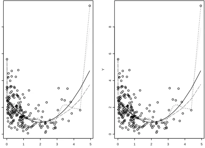
We illustrate our method with two sets of simulated data, one each from IID and autoregressive models, as well as a real-life dataset on hardwood sapling height-growth:
IID data. HereX1, . . . , Xnare generated as iid Exponential with expectation 1, and we consider
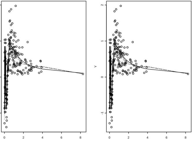
two models for Y1, . . . , Yn: a) Yi = 0.5(6−4Xi+Xi2)εi; b) Yi = sin(1/Xi)εi, 1≤i≤ n. Here
εi, 1≤i≤n, are taken to be i.i.d Weibull (1,2), i.e., with densityg(ε) = 2εexp(−ε2), ε≥0.
Figure-1 and Figure-2 illustrate our estimator for Model-a and Model-b respectively, and also provides a comparison with the usual kernel estimator. In both the figures we take n= 200, v= cn−1/5 forc= 0.2,0.5 and the perturbation-parameter²= 0 on the plot on theleft,²= 0.5v2 on
theright. The choice of ²is based on the relation²=O(v2) established in Chaubeyet al. (2007)
for density estimation. The kernel estimator is based on the standard Normal kernel, where the bandwidth is chosen to beh= 0.5n−1/5.
Figure-1 (Model-a) shows that ˜mn(·) with a lowv= 0.2n−1/5is affected by noisy observations,
as is the standard Normal kernel estimator, even with a high bandwidth. However, ˜mn with a
high v= 0.5n−1/5 adapts well to the shape of the true regression. Moreover, the right-hand plot
in Figure-1 shows that the effect of the large outlier near zero is reduced as ² is changed from zero to 0.5v2.In Figure-2 (Model-b) all the estimators are comparable.
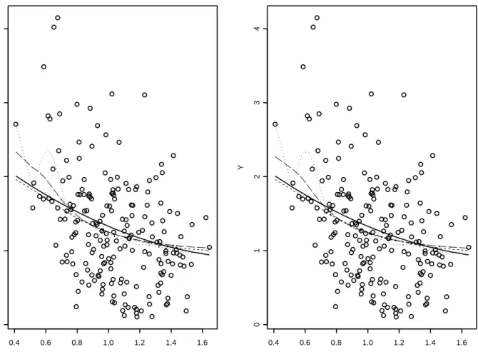
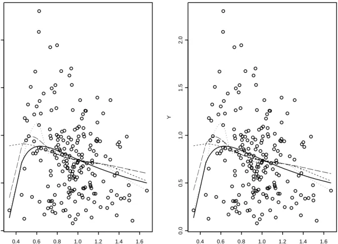
Autoregressive data. HereX1, . . . , Xn are generated as:
Xi = 0.5Xi−1+ (
q
0.2 + 0.1X2
i−1)εi, X0 Exponential (1),
wheren= 200, εi, 1≤i≤n,are i.i.d Weibull (1,3), i.e., with densityg(ε) = 3ε2exp(−ε3), ε≥0.
The two models forY1, . . . , Yn,as well as the choice of smoothing parameters and kernel function,
are exactly the same as the i.i.d case above. The illustration/comparison is provided in Figure-3 and Figure-4 for Model-a and Model-b respectively. The choice of v, ² here are the same as in the IID case above.
Figure-3 shows that ˜mn(·) with a low v = 0.2n−1/5 is affected by noisy observations, as in
the IID case. However, the standard Normal kernel estimator and ˜mn(·) with v = 0.5n−1/5 are
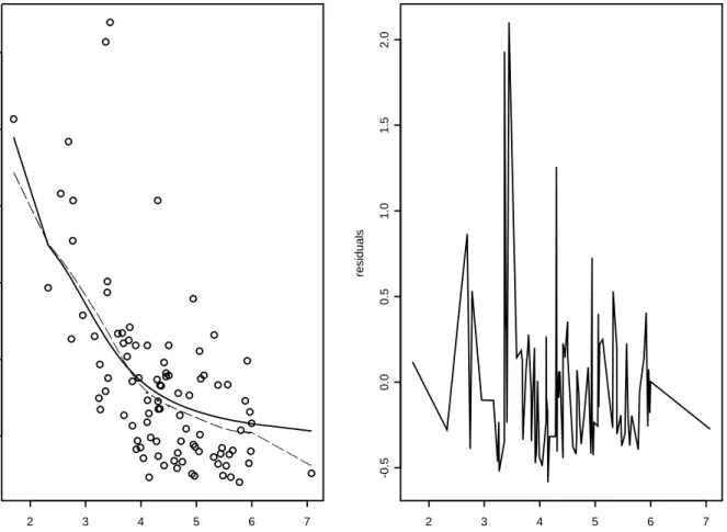
comparable in this case. In Figure-4 ˜mn(·) with low as well as highvdetect the shape of the true regression quite well, while the kernel estimator remains essentially flat over the entire range. Hardwood sapling data. We apply our method to data on initial height (X) versus 5-year height-growth (Y) of naturally-occurring hardwood saplings in gap areas of the boreal forest around Lake Duparquet in north-western Quebec. Both the initial height (as of 1998) and the height-growth (over 1998–2003) were obtained from multi-temporal LIDAR (LIght Detection And Ranging) surveys. (Data courtesy: Prof. Benoit St-Onge and Ms. Udayalakshmi Vepakomma, University of Quebec at Montreal.) All measurements are in meters, and the sample consists of n= 94 saplings.
Figure-5(a) gives the scatter-plot and our estimator ˜mn(·) along with the Standard Normal
kernel estimator for comparison. The bandwidth and perturbation-parameters (v, ²) for our estimator, as well as the bandwidth for the kernel estimator, were chosen by trial-and-error through visual inspection of the fitted lines and the residuals (Figure-5(b)). We would like to mention two points: firstly, the kernel estimator required a bandwidth (2.8n−1/5) that is 7 times that ofv= 0.4n−1/5 of ˜mn(·) for a comparably smooth fit; this indicates robustness of ˜mn(·)
vis-a-vis the kernel estimator. Secondly, ˜mn(·) captures quite clearly the stabilization (i.e., approaching a constant level) of growth as initial height — an indicator of age — increases, as is to be expected, whereas the kernel estimator shows a downward trend.
n=200, epsilon=0 X Y 0 1 2 3 4 5 0 2 4 6 8 n=200, epsilon=0.5*v^2 X Y 0 1 2 3 4 5 0 2 4 6 8
Figure 1: scatterplot and regression estimators for IID data with Y = 0.5(6−4X+X2)ε: true
regression (—), ˜mnwithv= 0.2n−1/5 (· · ·), ˜m
nwithv= 0.5n−1/5 (– –), standard Normal kernel
n=200, epsilon=0 X Y 0 2 4 6 8 -1 0 1 2 n=200, epsilon=0.5*v^2 X Y 0 2 4 6 8 -1 0 1 2
Figure 2: scatterplot and regression estimators for IID data withY = sin(1/X)ε: true regression (—), ˜mn with v = 0.2n−1/5 (· · ·), ˜m
n with v = 0.5n−1/5 (– –), standard Normal kernel with
n=200, epsilon=0 X Y 0.4 0.6 0.8 1.0 1.2 1.4 1.6 0 1 2 3 4 n=200, epsilon=0.5*v^2 X Y 0.4 0.6 0.8 1.0 1.2 1.4 1.6 0 1 2 3 4
Figure 3: scatterplot and regression estimators for autoregressive data withY = 0.5(6−4X+X2)ε:
true regression (—), ˜mn withv= 0.2n−1/5 (· · ·), ˜m
n withv = 0.5n−1/5 (– –), standard Normal
n=200, epsilon=0 X Y 0.4 0.6 0.8 1.0 1.2 1.4 1.6 0.0 0.5 1.0 1.5 2.0 n=200, epsilon=0.5*v^2 X Y 0.4 0.6 0.8 1.0 1.2 1.4 1.6 0.0 0.5 1.0 1.5 2.0
Figure 4: scatterplot and regression estimators for autoregressive data withY = sin(1/X)ε: true regression (—), ˜mnwithv= 0.2n−1/5 (· · ·), ˜m
nwithv= 0.5n−1/5 (– –), standard Normal kernel
(a) initial height growth 2 3 4 5 6 7 0.5 1.0 1.5 2.0 2.5 3.0 (b) initial height residuals 2 3 4 5 6 7 -0.5 0.0 0.5 1.0 1.5 2.0
Figure 5: scatterplot and regression estimators for height-growth data: (a) ˜mn with v =
0.4n−1/5, ² = 0.5v2 (—), standard Normal kernel with h = 2.8n−1/5 (– –); (b) line-plot of
residuals corresponding to ˜mn
Acknowledgements: The authors gratefully acknowledge financial support from the Statistical Laboratory of CRM, Montreal (for N.Laib’s trip to Montreal) and the NSERC Discovery grants (Y.Chaubey and A.Sen). The data-set used for illustration in Section 6 was kindly provided by B.St-Onge and U.Vepakomma of the UQAM.
7
Appendix: Proofs
This section gives detailed proofs. We start by two lemmas that we will be used in the sequel. Lemma B (La¨ıb 1999). Let {(Xi,Si) :i ≥1} be a sequence of martingale difference such that
|Xi| ≤B a.s. for 1≤i≤n. For all ² >0, one has P 1max≤i≤n ¯ ¯ ¯ i X j=1 Xj ¯ ¯ ¯> ² ≤2 exp µ − ²2 2nB2 ¶ .
Lemma C (Wu, 2003). For any y ∈ Rd let H n(y) =
Pn
i=1f(y|Fi)−nf(y). Then condition
(3.2) implies that supykHn(y)k22 =O(n).
In order to prove our results introduce some notations. For x ∈ [a, b], let x+ = x +² n,
an =a+²n and bn =b+²n. Let h(x) =m(x)f(x) and ˜mn(x) =mn(x+²n) := mn(x+). The
estimator ˜mn(x) ofm(x) can be written as
˜ mn(x) = hn(x+) fn(x+) , where hn(x+) = n1 n X i=1 φ(Yi)Qx+²n,vn(Xi) and fn(x+) = 1 n n X i=1 Qx+²n,vn(Xi). (7.1) Let hn(x+) = 1 n n X i=1 E[φ(Yi)Qx+²n,vn(Xi)| Fi−1] and fn(x+) = 1 n n X i=1 E[Qx+²n,vn(Xi)| Fi−1].(7.2)
We define the centralizing parameter ˜ Bn(x) := £ hn(x+)−h(x) ¤ −m(x)£fn(x+)−f(x)¤ fn(x+) (7.3)
for the “bias” of ˜mn(x). Then
˜ mn(x)−m(x)−B˜n(x) = f 1 n(x+) £ (hn(x+)−hn(x+)) −(m(x) + ˜Bn(x))(fn(x+)−fn(x+)) i , (7.4)
so that ˜Bn(·) can be viewed as the “asymptotic bias” of ˜mn(·). The major thrust of the
decom-position (7.4) is due to the fact that the summands of the term form a martingale difference. We state and prove now the following results which give the uniform convergence of the bias term.
Proposition 1 Assuming (A0)-(A4) hold, then we have sup x∈[a,b] ¯ ¯ ¯B˜n(x) ¯ ¯ ¯= 0 a.s. as n→+∞.
Proof of Proposition 1. It suffices to show that hn(x+)−h(x) converges uniformly in x to 0
and fn(x+) is uniformly bounded over. Making use of (A4) and the law of iterated conditional
expectation we can written
Thus, |hn(x+)−h(x)| ≤ ¯ ¯ ¯ ¯ ¯ 1 n n X i=1 Z R+ Qx+²n,vn(t)m(t)f(t|Fi−1)dt−h(x) ¯ ¯ ¯ ¯ ¯ ≤ ° ° ° ° ° 1 n n X i=1 f(·|Fi−1)−f ° ° ° ° ° Z R+Qx+²n,vn(t)m(t)dt+ ¯ ¯ ¯ ¯ Z R+Qx+²n,vn(t)h(t)dt−h(x) ¯ ¯ ¯ ¯. (7.5) By the Hille’s Lemma and (A0), the second integral goes to 0 uniformly inx. The first term is bounded above by ° ° ° ° ° 1 n n X i=1 f(·|Fi−1)−f ° ° ° ° °.xsup∈R+ |m(x)|,
which goes to 0 as n → ∞ in view of (A2) and the fact that m(·) is bounded. By the same arguments we can conclude by Hille’s Lemma, (A0) and (A2) that fn(x+) converges uniformly
inx tof(x) which is bounded over uniformly inx in view of (A3). ¤
The following Proposition gives an asymptotic lower bound for infx∈J|fn(x+)|.
Proposition 2 Assuming (A0)-(A3) hold, then we have
(i) sup x∈J |fn(x+)−f(x)|= 0 a.s. as n→ ∞ (ii) inf x∈Jfn(x +)>0 a.s as n→ ∞.
Proof of Proposition 2. For (i) we have
|fn(x+)−f(x)| ≤ |fn(x+)−fn(x+)|+|fn(x+)−f(x)|.
Making use of the same argument to prove Proposition 1, we can easily seen that the second term in the right hand side of the above inequality tends to 0 asn→ ∞. The first term converges also uniformly in x to 0 by the same arguments that used to prove Proposition 3 below. For (ii), we have for any x∈J,
inf
x∈J|fn(x
+)| ≥ inf
x∈Jf(x)−supx∈J|fn(x
+)−f(x)|.
Then (ii) follows from (i) and condition (A3). ¤
The main task now is to establish the uniform almost sure convergence for hn(x+)−h(x).
Making use of the Stirling’s formula we can easily seen that, for any fixed x, the function t 7→ Qx+²n,vn(t) is bounded above by √2π(x+²1 n)vn for every t≥0 whenever vn→ 0. By contrast, the
functionφ(y) is not necessarily bounded, it can thus be handled by a suitable truncation. To this end, let Mn =
n
nlnn[ln lnn]1+ζ o1/γ
, where ζ is a positive constant and γ is as in (A5). Note that the series PnMn is convergent. Let us now define the following processes
hbn(x+) = 1 n
n
X
i=1
hb n(x+) = 1 n n X i=1 E[φ(Yi)I{|φ(Yi)| ≤Mn}Qx+²n,vn(Xi)|Fi−1], (7.7)
where I stands for the indicator function. We have
hn(x+)−hn(x+) = (hn(x+)−hbn(x+)) + (hnb(x+)−hbn(x+)) + (hbn(x+)−hn(x+)).(7.8)
The asymptotic behavior of the three terms on the right hand side of (7.8) is given in the following results.
Lemma 1 Assuming (A5) holds, then, for each ω outside a null set D, there exists a positive integer n0(ω) such thathn(x+) =hbn(x+) for n≥n0(ω) and all x∈R+d.
Proof of Lemma 1. The proof uses the summability ofMn−γ and arguments similar to those used
by Roussas (1990). ¤
We deal now with the asymptotic behavior of the third term in (7.8). Lemma 2 Assuming (A2) and (A5) hold, then we have
sup x∈R+|h b n(x+)−hn(x+)|=O ¡ Mn1−γ¢ a.s. as n→ ∞. (7.9)
Proof of Lemma 2. We have by (A5) and the properties of conditional expectation that E[φ(Yi)Qx+²n,vn(Xi)I{Yi > Mn|}] ≤ Mn1−γE[|φ(Yi)|γQx+²n,vn(Xi)|Fi−1] = Mn1−γE[Qx+²n,vn(Xi)E[|φ(Yi)|γ|Gi−1]|Fi−1] ≤ Mn1−γ max 1≤i≤nE(|φ(Yi)| γG i−1)E[Qx+²n,vn(Xi)|Fi−1] ≤ CMn1−γ Z R+ Qx+²n,vn(t)f(t|Fi−1)dt. (7.10) Therefore, |hb n(x+)−hn(x+)| ≤ CMn1−γ ( k1 n n X i=1 f(·|Fi−1)−f(·)k Z R+ Qx+²n,vn(t)dt + Z R+ Qx+²n,vn(t)f(t)dt ¾ . (7.11)
The first member of (7.11) goes uniformly inxto 0 in view of (A2). The second one converges also uniformly inx, by Hille’s Lemma and (A0), tof(x) which is bounded. These imply (7.9). ¤
We study now the convergence of the main middle term on the right side of (7.8). Proposition 3 Let νn be a sequence of real number such that
νn→ ∞ and µ an b2 n ¶vn Mnvn−3νn−1 →0 as n→ ∞. (7.12)
Assuming (A0) holds and for any λ >0 X n≥1 νnexp ¡ −a2nπλ2nMn−2vn2¢<∞. (7.13) Then, we have sup x∈[a,b] |hbn(x+)−hb n(x+)|= 0 a.s. as n→ ∞. (7.14)
Remark 2. The condition (7.12) is satisfied if we choose, for instance,νn=
h³ an b2 n ´vn Mnvn−3logn i + 1 whereas (7.13) holds true by takingλ=λn=√Cn Mn
an√πnvn, whereCis a large positive constant.
Proof of proposition 3. Divide the interval [a, b] into subintervals each of lengthδn= (b−a)/νn.
Since the setJn={x;|x| ≤ |b−a|}is compact, it can be covered by a finite number of bounded
intervals with centersxnj whose sides are of length δn. That isJ = [a, b] =Sνn
j=1Jnj,where Jnj = © x; |x−xnj| ≤(b−a)νn−1 ª , j= 1, . . . , νn. (7.15)
Let Vn(x+) =hbn(x+)−hbn(x+), then we have, forxnj ∈Jnj, that
sup x∈J |Vn(x+)| = max 1≤j≤νn sup x∈J∩Jnj |Vn(x+)| ≤ max 1≤j≤νn sup x∈J∩Jnj |Vn(x+)−Vn(x+nj)|+ max1≤j≤ν n |Vn(x+nj)| := T1n+T2n+T3n, where T1n = max 1≤j≤νn sup x∈Jn∩Jnj |hbn(x+)−hbn(x+nj)| (7.16) T2n = max 1≤j≤νn sup x∈Jn∩Jnj |hb n(x+)−hbn(x+nj)| (7.17) T3n = max 1≤j≤νn |hbn(x+nj)−hb n(x+nj)|. (7.18)
In order to give an upper bound of each term in the above inequalities we have to establish the following Lemmas.
Lemma 3 Under (A0) we have (i) T1n=O(ξn)
(ii) T2n=O(ξn) with ξn=C1a−n4
µ b2 n an ¶αn α3/2n Mn.νn−1
Proof of Lemma 3. We prove only (i), the proof of (ii) is similar. We have
|hbn(x+)−hbn(x+nj)| ≤ 1 n n X i=1 |φ(Yi)|I{|φ(Yi)| ≤Mn} ¯ ¯Qx+² n,vn(Xi)−Qxnj+²n,vn(Xi) ¯ ¯.
Now observe that Qx+²n,vn(Xi)−Qxnj+²n,vn(Xi) = Xiαn−1 Γ(αn) e−αnXi/x + βαn x+ − e −αnXi/x+nj βαn x+nj , (7.19) where βα x+ = (vn2x+)α and αn= v12
n.The term in brackets in (7.19) can be written as
e−αnXi/x+ −e−αnXi/x+nj βαn x+ + µ βαn x+nj −β αn x+ ¶ e−αnXi/x+nj βαn x+. βαx+n nj . (7.20)
Since forc >0 and for any t, (0< a0 ≤t ≤b), the function fc(t) =e−c/t is a Kc lipshitz of
order one withKc= ac2 0e
−c/b, it follows, for all x, xj
n∈[a, b], that
|e−αnXi/x+ −e−αnXi/x+nj| ≤ α2nXi2e−αnXi/bn
a2 nx+ x+nj
|x−xnj|. (7.21)
Moreover, making use of the mean value theorem, we can write, for x∗ betweenx+ and x+ nj, that |βαn x+ −βαx+n nj | ≤ αnvn2αn|x−xnj|xα∗n−1 ≤ bαnn−1αnvn2αn|x−xnj|. (7.22)
Combining (7.20), (7.21) and (7.22) we can then bound above the right hand of (7.19) by |Qx+²n,vn(Xi)−Qxnj+²n,vn(Xi)| (7.23) ≤ · 1 a4 n βαn bn βαn an α2nXαn+1 i Qb+²n,vn(Xi) + αnvn2αnbnαn−1 βαn an Xiαn−1Qa+²n,vn(Xi) ¸ |xi−xnj| ≤ · 1 a4 n µ bn an ¶αn α2nXαn+1 i Qb+²n,vn(Xi) +αnbαnn−1a−n2αnX αn−1 i Qa+²n,vn(Xi) ¸ |xi−xnj|.
Making use of the Stirling’s formula, we can see, for x fixed and τ ≥ 0, that the function t7→tτQ
x+²n,vn(t) is bounded above by
(x+²√n)τ−1
2πvn whenever vn→0. It follows that
|Qx+²n,vn(Xi)−Qxnj+²n,vn(Xi)| ≤ 1 +a4n a4 n √ 2π µ b2n an ¶αn v−n3|x−xnj|. (7.24) Hence, T1n≤(b−a)1 +a 4 n a4 n √ 2π µ b2 n an ¶αn v−n3Mnνn−1=O(ξn) (7.25)
This completes the proof of Lemma 3. ¤
Lemma 4 Suppose that (A0) holds and that X n νnexp ¡ −anπλ2nv2nMn−2 ¢ <∞. (7.26) Then we have T3n= 0 a.s as n→ ∞. (7.27)
Proof of Lemma 4. The proof uses Lemma B. To this end write|hb
n(x+nj)−hbn(x+nj)|=
Pn
i=1Ln(x+nj),
where Ln(x+nj) = n1{φ(Yi)I{|φ(Yi)| ≤Mn}Qxnj+²n,vn(Xi).It is clear, for xnj ∈[a, b], that
|Ln(x+nj)| ≤ 1 √ 2πx+njvn n−1Mn≤ √ 1 2πanvn n−1Mn,
whenever vn→0. Moreover, for any fixedj, 1≤j ≤νn,
³
Ln(x+nj),Fi
´
is a bounded martingale difference, we can then apply Lemma B, to get for any λ >0
P{T3n≥λ} ≤2νnexp¡−anπλ2nv2nMn−2¢. (7.28) The result follows from Borel Cantelli’s Lemma and condition (7.26). ¤
Proof of Theorem 1. The proof follows from decomposition (7.4), Propositions 1 to 3 and Lemmas 1 to 4. ¤.
Proof of Theorem 2.
(i) We have from (7.4) that for anyx >0 √ nvn ³ ˜ mn(x)−m(x)−B˜n(x) ´ = Rn(x+) fn(x+) −An(x +), (7.29) where Rn(x+) = √nvn ¡ (hn(x+)−hn(x+))−m(x)(fn(x+)−fn(x+)) ¢ An(x+) = √ nvn ˜ Bn(x)(fn(x+)−fn(x+)) fn(x+) . Let ηni= ³v n n ´1/2 [(φ(Yi)−m(x))Qx+²n,vn(Xi)] and ξni =ηni−E[ηni|Fi−1]. Then Rn(x+) = Pn
i=1ξni. Once the asymptotic normality of Rn(x+) is established, that of
˜
mn(x)−m(x)−B˜n(x) follows fromAn(x+)→0 in probability andf
n(x+)→f(x) in probability
asn→ ∞.
Lemma 5 below gives convergence in probability offn(x+) to f(x).
Proof of Lemma 5. The result follows from a direct applications of Hille’s Lemma combining with Lemma B.¤
The following lemma gives the asymptotic behavior ofAn(x+).
Lemma 6 Assuming (A0)-(A3) hold. Iff(x)>0 at a given x∈R+
∗, then we have
An(x+) =oP(1) as n→ ∞.
Proof of Lemma 6. Arguing as in the proof of Proposition 4 below by letting m(x) = 0 and φ(Yi) ≡1, we get for any x >0, under condition (7.30), the following central limit theorem for
the density estimator, √ nvn(fn(x+)−fn(x+)→ ND µ 0, f(x) 2√πx ¶ .
Thus,fn(x+)−fn(x+) =OP(1/√nvn). It follows from Lemma 5 that An(x+) =OP(1)|B˜n(x)|.
We conclude by Proposition 1 that An(x+) =oP(1). ¤
Proposition 4 LetW2+δ(Xi) =E[φ2(Yi)|Gi−1]be derivable atX=xfor someδ >0and assume
that W2+δ(x) is bounded at a neighborhood of x. Moreover suppose that
nvn→ ∞ as n→ ∞ and max
1≤i≤nsupt f(t|Fi−1)<∞. (7.30)
Then we have for a given x∈R∗ + that Rn(x+)→ ND ¡ 0, τ2(x)¢, where τ2(x) = f(x) 2√πx(W2(x)−m 2(x)). (7.31)
Proof of Proposition 4. Observe that for any fixedx, the summands inRn(x+) form a triangular
array stationary martingale differences with respect the sigma field Fi−1, we can then apply a
CLT for discrete-time arrays of real-valued martingales, as given for instance in Hall and Heyde (1980), to prove the asymptotic normality ofRn(x+). It suffices then to prove
Pn i=1E £ ξ2 ni|Fi−1 ¤ P
−→τ2(x) and the Lindeberg condition
nE£ξ2
niI[|ξni|>ε]
¤
=o(1) holds for anyε >0.
In order to prove the first statement making use of condition (7.30) and the fact that m(·) is bounded, one get
|E[ηni|Fi−1]| = ³v n n ´1/2 E[(m(Xi)−m(x))Qx+²n,vn(Xi)|Fi−1] = ³v n n ´1/2Z R+∗ (m(t)−m(x))Qx+²n,vn(t)f(t|Fi−1)dt ≤ C ³v n n ´1/2 , where C= maxisuptm(t)f(t|Fi−1).Thus
¯ ¯ ¯ ¯ ¯ n X i=1 E£η2ni|Fi−1 ¤ − n X i=1 E£ξni2 |Fi−1 ¤¯¯¯ ¯ ¯ ≤ n X i=1 (E[ηni|Fi−1])2 ≤ C2.vn→0 as n→ ∞. (7.32)
Consequently, we have only to prove n X i=1 E£η2ni|Fi−1 ¤ P −→τ2(x). (7.33)
Observe now that
n X i=1 E£η2ni|Fi−1 ¤ = vn n n X i=1 E£W2(Xi)Q2x+²n,vn(Xi)|Fi−1 ¤ −vn n n X i=1 E£m(x)(2m(Xi)−m(x))Q2x+²n,vn(Xi)|Fi−1 ¤ = J1n+J2n. (7.34)
The termJ1n can be be split as follows
J1n=vn Z R+∗ W2(t)Q2x+²n,vn(t) " 1 n n X i=1 f(t|Fi−1)−f(t) # dt+vn Z R+∗ W2(t)Q2x+²n,vn(t)f(t)dt.(7.35) By (A2) the term in brackets in (7.35) goes to 0 uniformly int. Moreover,vn
R R+∗ W2(t)Q 2 x+²n,vn(t)dt is bounded above by vnsup t Qx+²n,vn(t) Z R+∗ W2(t)Qx+²n,vn(t)dt≈ 1 √ 2πxW2(x) since by Hille’s Lemma RR∗
+W2(t)Qx+²n,vn(t)dt →W2(x). This implies that the first member in Jn1 goes to 0 asn→0. The second member in (7.35) can be split as
vn Z R∗ + (W2(t)f(t)−W2(x)f(x)Q2x+²n,vn(t)dt+vn Z R∗ + W2(x)f(x)Q2x+²n,vn(t)dt. (7.36)
Making use of a Taylor expansion of order one of the function t7→(W2f)(·) and the fact that
Z ∞ 0 tpQmx+²n,vn(t)dt= ( 1 v2x+)m/v 2 ¡ m v2x+ ¢((m/v2)+p+1−m). Γ(m/v2+p+ 1−m) Γm(1/v2) ≈ p 1 m(2π)m−1 1 vm−1(x+² n)m−p−1 1 q 1−v2(m−p−1 m ) , asv→0, (7.37)
one can show that the first member in (7.36) tends to 0. Moreover, the second one is asymptoti-cally equivalent, as²n→0, to
Jn1 ≈ f(x)W2√π x2(x). (7.38)
Jn2 = −vn Z R+∗ (2m(t)−m(x)[n−1 n X i=1 f(t|Fi−1)−f(t)]dt − vnm(x) Z R+∗ (m(t)−m(x))Q2x+²n,vn(t)f(t)dt − vnm(x) Z R+ ∗ (m(t)f(x)−m(x)f(x))Q2x+²n,vn(t)f(t)dt − vnm(x)2f(x) Z R+∗ Q2x+²n,vn(t)dt. (7.39)
Using the same argument as above we can easily seen that Jn2 is asymptotically equivalent, as ²n→0, to
Jn2≈ −f(x)m 2(x)
2√π x . (7.40)
Then (7.33) follows from (7.38) and (7.40).
The Lindeberg condition results from Corollary 9.5.2 in Chow and Teicher (1998) which implies that nE[ξ2
niI(|ξni|> ²)]≤4nE[η2niI(|ηni|> ε/2)].
Leta >1 and b >1 such that 1a+1b = 1. Making use of H¨older and Markov inequalities one can write for all ε >0
E[ηni2 I(|ηni|> ε/2)]≤ E|ηni| 2a
(ε/2)2a/b.
Taking 2a= 2 +δ we get
4nE[η2niI(|ηni|> ε/2)] =O(1).n−δvn(2+δ)/2.E[|(φ(Yi)−m(x))Qx+²n,vn|2+δ]
≤ O(1).n−δ/2v(2+δ)/2n h E(φ(Yi)Qx+²n,vn(Xi))2+δ+E(m(x)Qx+²n,vn)2+δ i = O(1).n−δ2v 2+δ 2 n "Z R∗ + W2+δ(t)Q2+δx+²n,vn(t)f(t)dt+m2+δ(x) Z R∗ + Q2+δx+²n,vn(t)f(t)dt # . (7.41)
The first term in (7.41) can be written as
O(1)n−δ2v 2+δ 2 n "Z R∗ + [W2+δ(t)f(t)−W2+δ(x)f(x)]Q2+δx+²n,vn(t)dt− Z R∗ + W2+δ(x)f(x)Q2+δx+²n,vn(t) # (7.42)
Using the approximation formula given in (7.37), we get
O(1)n−δ/2vn(2+δ)/2 "Z R∗ + W2+δ(x)f(x)Q2+δx+²n,vn(t) # =O(1)(nvn)−δ/2→0 as n→ ∞. (7.43)
sincenvn→ ∞asn→ ∞. By the continuity of the functiont→W2+δ(t)f(t) one can show that
the first member in (7.42) also goes to 0 asn→ ∞. Similarly one can show that the second term in (7.41) is asymptotically negligible. This completes the proof of part (i).
Part (ii). To prove (ii) we need to give an estimate of the convergence rate in probability of the bias term. This is the subject of the following lemma.
Lemma 7 Suppose that (A0)-(A4) hold and the condition (3.2) is satisfied. Moreover, assuming that f and m have bounded derivatives up to order two. Then we have
|B˜n(x)|=OP ¡ max¡max(v2n, ²n ¢ , n−1)¢=OP ¡ max(vn2, ²n) ¢ . (7.44)
Proof of Lemma 7. From (7.3), it suffices to give a convergence rate of hn(x+)−h(x). To this
end write
hn(x+)−h(x) = ¡hn(x+)−Ehn(x+)¢+¡Ehn(x+)−h(x)¢. (7.45) Making use of (A4) one may write
hn(x+)−Ehn(x+) = n1 Z R+ m(t)Qx+²n(t) " n X i=1 f(t | Fi−1)−nf(t) # dt = 1 n Z R+m(t)Qx+²n, vn(t)Hn(t)dt, (7.46) whereHn(t) = Pn
i=1f(t |Fi−1)−nf(t). We have then by Cauchy inequality and Lemma C that
Eh¯¯hn(x+)−Ehn(x+) ¯ ¯2i ≤ 1 n2. £ E¡Hn2(t)¢¤ µZ R+m(t)Qx+²n(t)dt ¶2 = O(n−1) µZ R+ m(t)Qx+²n(t)dt ¶2 . (7.47)
In order to deal with the second term in (7.47) recall thatQx+²n,vn(t) = 1 x+²ngα,β(
t
x+²n),where
gα,β(·) stands for the probability density function of the gamma distribution parameterized in terms of a shape parameter α and inverse scale parameter β =α=v2
n, which in turn, has mean
equals 1 and variancev2
n. Thus, we have, by a Taylor expansion one get
Z ∞ 0 Qx+²n,vn(t)m(t)dt= Z ∞ 0 gα,β(s)m((x+²n)s)ds = Z ∞ 0 gα,β(s)[m(x) + (x(s−1) +s²n))m0(x) +(x(s−1) +s²n)) 2 2 m 00(x) +O ³ (x(s−1) +s²n))2 ´ ]ds = O(1) +O(vn2) +O(²n) +O
¡ max(v2n, ²n) ¢ =O(1) +O¡max(vn2, ²n) ¢ =O(1). (7.48) ThusEh¯¯hn(x+)−Ehn(x+) ¯ ¯2i
=O(n−1).By the same argument as above one can see that
(Ehn(x+)−h(x)) =O
¡ max(v2
n, ²n)
¢
. These leads to the desired result. Part (iii). The proof is similar of part (ii). ¤.
Proof of theorem 3. We only give the proof when d = 2. The proof of Lemma 5 and Lemma 6 still unchanging since the Hille’s Lemma and Lemma A are also true on R+d. Let g now be a
function defined onR+dposses continuous bounded partial derivatives of order one at each point
of an open set S ⊂ R+d. Then for each point (s, t), (s, t) 6= (x+²
n1, y+²n2) := (x+, y+), such
that the line segment L((s, t),(x+, y+)) joining (s, t) and (x+, y+) in S, we have
Z
R+dg(s, t)Q
2
where I1n = Z R+d[g(s, t)−g(x +, y+)]Q2 (x+²n1,y+²n2),v(s, t)dsdt ≈ Z R+d · (s−x+) ∂g ∂x+(x+, y+)−(t−y+) ∂g ∂y+(x+, y+) ¸ Q2x+²n1,v(s)Q2y+²n2,v(t)dsdt→0, asn→ ∞,in view of the approximation formula (7.37) whenever the partial derivatives ofg are bounded. Using again the approximation formula (7.37) and the continuity of g, we get
I2n = Z R+dg(x +, y+)Q2 (x+²n1,y+²n2),v(s, t)dsdt≈g(x, y) 1 4πv2xy as (²n1, ²n2)→(0,0).
It suffices then to replace in the proof of proposition 4, vn by vd
n and to apply the above
result with g(s, t) = W2(s, t)f(s, t) in (7.36) and g(s, t) = m(s, t)f(s, t) in (7.39) and finally
g(s, t) =W2+δ(s, t)f(s, t) in (7.42). ¤
References
Andrews, D.W.K., 1984. Non-strong mixing autoregressive processes. J. Appl. Probab. 21, 930-934. Bagai, I. and Prakasa Rao, B.L.S. (1996). Kernel type density estimates for positive valued random
variables. Sankhya. A57, 56-67.
Bosq, D., 1998. Nonparametric Statistics for Stochastic Processes. Lecture Note in Statistics. Springer, New York.
Bouezmarni, T. and Scaillet, O. (2005). Consistency of asymmetric kernel density estimators and smoothed histograms with application to income data. Econometric Theory21, 390-412.
Chanda, K.C., 1974. Strong mixing of linear stochastic processes. J. Appl. Probab. 11, 401-408. Chaubey, Y.P., Sen, A. and Sen, P.K. (2007). A new smooth density estimator for non-negative random
variables. Submitted.
Chaubey, Y.P. and Sen, P.K. (1996). On smooth estimation of survival and density functions. Statist. Decisions14, 1-22.
Chen, S.X. (1999). Beta kernel estimators for density functions. Comput. Statist. Data Anal. 31, 131-145.
Chernick, M.R., 1981. A limit theorem for the maximum of autoregressive processes with uniform marginal distributions. Ann. Probab. 9, 145-149.
Chow, Y.S. and Teicher, H. (1998). Probabilty Theory, 2nd ed. Springer, New York.
Feller, W. (1965). An Introduction to Probability Theory and its Applications, Vol II. New York: John Wiley and Sons.
Diaconis, P. and Freedman, D. (1999). Iterated random functions. SIAM Rev. 41, 41-76.
Engle, R.F., 1982. Autoregressive conditional heteroscedasticity with estimates of the variance of United Kingdom inflation. Econometrica. 50, 987-1007.
Gasser, T. and M¨uller, H.G. (1979). Kernel estimation of regression functions. In: Smoothing Techniques for Curve Estimation, eds. Gasser and Rosenblatt. Heidelberg: Springer-Verlag.
Gu´egan, D., Ladoucette, S., 2001. Non-mixing properties of long memory processes. C. R. Acad. Sci. Paris, 333, 373-376.