Oracally Efficient Two-Step Estimation of Generalized Additive Model

SFB 649 Discussion Paper 2011-016

Oracally Efficient Two-Step

Estimation of Generalized

Additive Model

Rong Liu*

Lijian Yang**

Wolfgang Karl Härdle***

* University of Toledo, USA ** Michigan State University, USA *** Humboldt-Universität zu Berlin, Germany

This research was supported by the Deutsche

Forschungsgemeinschaft through the SFB 649 "Economic Risk". http://sfb649.wiwi.hu-berlin.de

ISSN 1860-5664

SFB 649, Humboldt-Universität zu Berlin Spandauer Straße 1, D-10178 Berlin

S

FB

6

4

9

E

C

O

N

O

M

I

C

R

I

S

K

B

E

R

L

I

N

ORACALLY EFFICIENT TWO-STEP ESTIMATION OF GENERALIZED ADDITIVE MODEL ∗

By Rong Liu1_{, Lijian Yang}2,3 _{and Wolfgang K. H¨ardle}4 1_{University of Toledo,}2_{Soochow University,} 3_{Michigan State University,}

4_{Humboldt-Universit¨at zu Berlin}

Generalized additive models (GAM) are multivariate nonpara-metric regressions for non-Gaussian responses including binary and count data. We propose a spline-backfitted kernel (SBK) estimator for the component functions. Our results are for weakly dependent data and we prove oracle efficiency. The SBK techniques is both com-putational expedient and theoretically reliable, thus usable for ana-lyzing high-dimensional time series. Inference can be made on com-ponent functions based on asymptotic normality. Simulation evidence strongly corroborates with the asymptotic theory.

1. Introduction. An effective semiparametric regression tool for high dimensional data is the additive model introduced byHastie and Tibshirani (1990), which stipulates that

(1.1) E(𝑌∣X) =𝑚(X), 𝑚(X) =𝑐+∑𝑑_𝛼=1𝑚𝛼(𝑋𝛼)

for a response 𝑌 and a predictor vector X = (𝑋1, ..., 𝑋𝑑)T. When a data

set {𝑌𝑖,XT_𝑖 }𝑛_𝑖=1 = {𝑌𝑖, 𝑋𝑖1, ..., 𝑋𝑖𝑑}𝑛𝑖=1 of size 𝑛 is observed which follows

model (1.1), unknown component functions{𝑚𝛼(𝑥𝛼)}𝑑_𝛼=1 can be estimated

via kernel, B spline and smoothing spline with a univariate convergence rate. This fact together with the interpretability of the functions has not only led to a remedy of the “curse of dimensionality”, but also led to in-creased practical applications of additive models. A list of articles on addi-tive models and related works include, among others, Stone (1985), Stone

(1994), Huang (2004) and Xue and Yang (2006a) for B spline methods;

Tjøstheim and Auestad (1994), Linton and Nielsen (1995), Linton (1997),

Fan et al.(1998),Yang et al.(1999),Xue and Yang(2006b) andYang et al.

∗_{Supported in part by the Deutsche Forschungsgemeinschaft through the CRC 649} “Economic Risk”, by NSF awards DMS 0706518, 1007594 and by a Credit Rating Grant from the National University of Singapore Risk Management Institute.

AMS 2000 subject classifications:Primary 62M10; secondary 62G08

JEL classification: C00, C14, J01, J31

Keywords and phrases:Bandwidths, B spline, knots, link function, mixing,

Nadaraya-Watson estimator

(2006) for kernel methods; and more recently, spline-backfitted kernel (SBK) smoothing methods ofWang and Yang(2007),Wang and Yang(2009),

Liu and Yang(2010) andMa and Yang (2011), the spline-backfitted spline

(SBS) smoothing method ofSong and Yang (2010).

Certain types of responses 𝑌, however, such as binary or Poisson re-sponses, are much more appropriately described by GAMs. In the GAM framework, the data{𝑌𝑖,XT𝑖

}_𝑛

𝑖=1 are generated according to

(1.2) E(𝑌∣X=x) =𝑏′_{𝑚(x)},

with𝑚(x) of additive structure as in (1.1), and a given function𝑏′ _which

re-lates𝑚(x) to the conditional variance function 𝜎2_{(x) =Var(𝑌∣X=x) via}

the equation 𝜎2_{(x) = 𝑎(𝜙)𝑏}′′_{{𝑚(x)}, in which𝑎(𝜙) is a nuisance}

param-eter that quantifies overdispersion. The inverse of 𝑏′ _{is called the link}

func-tion. For binary responses, one commonly takes (𝑏′₎−1_{(𝑥) = log{𝑥/(1−𝑥)},}

the logistic link to conduct logistic regression, while for Poisson regression, (𝑏′₎−1_{(𝑥) = log𝑥, the log link. If one takes (𝑏}′₎−1_{(𝑥) =𝑥, the identity link,}

model (1.2) becomes model (1.1).

Model (1.2) has its origin in the special case where the probability density function of 𝑌𝑖 conditional on X𝑖 with respect to a fixed 𝜎-finite measure

forms an exponential family

𝑓(𝑌𝑖∣X𝑖, 𝜙) = exp [{𝑌𝑖𝑚(X𝑖)−𝑏{𝑚(X𝑖)}}/𝑎(𝜙) +ℎ(𝑌𝑖, 𝜙)].

For the theoretical development in this paper, however, it is not necessary to assume that the data {𝑌𝑖,XT𝑖

}_𝑛

𝑖=1 comes from such exponential family,

but only that the conditional variance and conditional mean are linked by the following equation

Var(𝑌∣X=x) =𝑎(𝜙)𝑏′′[(𝑏′)−1{E(𝑌∣X=x)}]. We can also write model (1.2) in the usual regression form (1.3) 𝑌𝑖 =𝑏′{𝑚(X𝑖)}+𝜎(X𝑖)𝜀𝑖

for conditional white noise𝜀𝑖 that satisfies E(𝜀𝑖∣X𝑖) = 0,E(𝜀2𝑖∣X𝑖)= 1. For

identifiability, one requires that

(1.4) E{𝑚𝛼(𝑋𝛼)}= 0,1≤𝛼≤𝑑

for unique additive representations of𝑚(x) =𝑐+∑𝑑_𝛼=1𝑚𝛼(𝑥𝛼). As in most

is conducted on compact sets. Without lose of generality, let the compact set be 𝝌= [0,1]𝑑.

Methods for the generalized additive model (1.2) are much less developed in comparison to the additive model (1.1), see for instance, the B spline method of Stone (1986) and Xue and Liang (2010), the kernel method of

Linton and H¨ardle (1996) andYang et al. (2003), and the two-stage

meth-ods ofHorowitz and Mammen(2004) andHorowitz et al.(2006). Generally speaking, the proposed kernel methods are too computationally intensive for high dimension𝑑, thus limiting their applicability to a small number of predictors. On the other hand, B spline methods provide only convergence rates but no asymptotic distributions, so no measures of confidence can be assigned to the estimators. In the case of the additive model (1.1), the SBK method of Wang and Yang (2007) combines the advantages of both kernel and spline methods and the result is balanced in terms of theory, computa-tion, and interpretation. The basic idea of the SBK method for the additive model (1.1) is to first project the data with B-splines into a space of func-tions with additive structure and then to apply kernel smoothing to the projected objects.

In this paper we extend the SBK method to model (1.2). The desired aim is to achieve orcale efficiency. If all the nonparametric functions of the last 𝑑−1 variables, {𝑚𝛼(𝑥𝛼)}𝑑𝛼=2 and the constant 𝑐 were known by an

“ora-cle”, one could simply plug these in and estimate the only unknown functions 𝑚1(𝑥1) by maximizing the log-likelihood function with kernel weights

com-puted from variable𝑋1. This estimator of𝑚1(𝑥1) is called “oracle smoother”

or “infeasible estimator”, and it does not suffer from the “curse of dimen-sionality” since the smoothing operation involves w.l.o.g. only𝑋1. The

pro-posed SBK method pre-estimates functions {𝑚𝛼(𝑥𝛼)}𝑑𝛼=2 and constant 𝑐

by linear splines and then use these estimates as proxies for the unknown functions {𝑚𝛼(𝑥𝛼)}𝑑_𝛼=2 and constant 𝑐. The main contribution is proving

that the error caused by this approximation is uniformly negligible of order

𝒪𝑎.𝑠.(𝑛−1/2log𝑛). Consequently, the SBK estimator is uniformly (over the

data range) asymptotically equivalent to the “oracle smoother”, automati-cally inheriting all oracle efficiency properties of the latter. Our proof relies on “reducing bias by undersmoothing” and “averaging out the variance”, accomplished with the joint asymptotics of kernel and spline functions for realizations of geometrically strongly mixing time series. These results are es-tablished under substantially greater technical difficulty than existng works on additive model such as Wang and Yang(2007), Wang and Yang(2009),

Liu and Yang(2010),Ma and Yang(2011), andSong and Yang(2010). The

esti-mation error into the sum of a bias and a noise term when the link function (𝑏′₎−1 _{is nonlinear.}

A similar result was proved in Horowitz and Mammen (2004) for i.i.d. rather than dependent data and only pointwise rates instead of uniform rates were derived. It is also worth emphasizing that althoughHorowitz and Mammen (2004) had used the B-spline estimator for the first stage in simulation, their proof is valid only for using the orthogonal series estimator in stage one. Another major contribution of this paper is establishing that the spline-backfitted estimator of the additive constant𝑐 is within an negligible error of order 𝒪𝑝(𝑛−1/2) of the infeasible estimator and thus also oracally

effi-cient. As far as we know, our estimator of the additive constant𝑐is the only one which has an asymptotic distribution with𝑛−1/2 _rate.

The paper is organized as follows. In Section 2 we discuss the assump-tions of the model (1.2). In Section 3, we introduce the oracle smoother or infeasible estimator for 𝑚1(𝑥1) and for 𝑐, and state their asymptotics. In

Section4we introduce the SBK estimator for𝑚1(𝑥1) and spline-backfitted

estimator for 𝑐 and present their asymptotic oracle efficiencies by showing that they differ from their infeasible counterparts only negligibly. In Section 5we describe implementation steps of the estimators. In Section6we apply the methods to simulated and real examples. All technical proofs are given in the Appendix.

2. Model assumptions. Following Stone (1985), p. 693, the space of 𝛼-centered square integrable functions on [0,1] is

ℋ0={𝑔:E{𝑔(𝑋𝛼)}= 0,E{𝑔2(𝑋𝛼)}<+∞}.

Next define the model space ℳ, a collection of functions onℝ𝑑 _as ℳ={𝑔(x) =𝑐+∑𝑑_𝛼=1𝑔𝛼(x) ;𝑔𝛼∈ ℋ0

}

,

in which𝑐is finite constant. The constraints thatE{𝑔𝛼(𝑋𝛼)}= 0, 1≤𝛼≤𝑑

ensure unique additive representation of 𝑚𝛼 as expressed in (1.4), but are

not necessary for the definition of spaceℳ. In what follows, denote byE𝑛

the empirical expectation, E𝑛𝜑=∑𝑛𝑖=1𝜑(X𝑖)/𝑛. We introduce two inner

products onℳ. For functions𝑔1, 𝑔2 ∈ ℳ, the theoretical and empirical inner

products are defined respectively as⟨𝑔1, 𝑔2⟩= E{𝑔1(X)𝑔2(X)},⟨𝑔1, 𝑔2⟩_𝑛= E𝑛{𝑔1(X)𝑔2(X)}. The corresponding induced norms are∥𝑔1∥22=E𝑔21(X), ∥𝑔1∥2_2,𝑛 =E𝑛𝑔21(X). More generally, we define ∥𝑔∥𝑟𝑟 =E𝑔𝑟(X).

Throughout the paper, for any compact interval [𝑎, 𝑏], we denote the space of𝑝-th order smooth function as𝐶(𝑝)_{[𝑎, 𝑏] =}{_𝑔∣𝑔(𝑝)_{∈𝐶[𝑎, 𝑏]}}_{, and the class}

of Lipschitz continuous functions for constant 𝐶 > 0 as Lip ([𝑎, 𝑏], 𝐶) =

{𝑔∣ ∣𝑔(𝑥)−𝑔(𝑥′_{)∣ ≤𝐶∣𝑥−𝑥}′_{∣,∀𝑥, 𝑥}′ _{∈[𝑎, 𝑏]}. We mean by “∼” both sides}

having the same order as 𝑛 → ∞. For any vector x = (𝑥1, 𝑥2,⋅ ⋅ ⋅, 𝑥𝑑)T,

we denote the supremum and 𝑝 norms as ∣x∣= max1≤𝛼≤𝑑∣𝑥𝛼∣ and ∥x∥_𝑝 = (∑_𝑑

𝛼=1𝑥𝑝𝛼 )_1/𝑝

. In particular, we use ∥x∥to denote the Euclidean norm. We need the following Assumptions on the data generating process. (A1) The additive component functions 𝑚𝛼 ∈ 𝐶(1)[0,1],1 ≤ 𝛼 ≤ 𝑑 with

𝑚1 ∈𝐶(2)[0,1], 𝑚′𝛼 ∈Lip ([0,1], 𝐶𝑚) = 2≤𝛼 ≤𝑑 for some constant

𝐶𝑚 >0.

(A2) The inverse link function 𝑏′ _{satisfies: 𝑏}′ _{∈ 𝐶}2_{(ℝ), 𝑏}′′_{(𝜃) > 0, 𝜃 ∈ ℝ} while for a compact interval Θ whose interior contains 𝑚([0,1]𝑑),

𝐶𝑏 >max𝜃∈Θ𝑏′′(𝜃)≥min𝜃∈Θ𝑏′′(𝜃)> 𝑐𝑏 for constants 𝐶𝑏> 𝑐𝑏>0.

(A3) The conditional variance function 𝜎2_{(x) is measurable and bounded.}

The errors {𝜀𝑖}𝑛_𝑖=1 satisfy E(𝜀𝑖∣ℱ𝑖) = 0, E (

∣𝜀𝑖∣2+𝜂 )

≤ 𝐶𝜂 for some

𝜂∈(1/2,1]and the sequence of 𝜎-fields

ℱ𝑖 =𝜎{(X𝑗), 𝑗 ≤𝑖;𝜀𝑗, 𝑗 ≤𝑖−1} for 𝑖= 1, . . . , 𝑛.

(A4) The density function 𝑓(x) of (𝑋1, ..., 𝑋𝑑) is continuous and

0< 𝑐𝑓 ≤infx∈𝝌𝑓(x)≤supx∈𝝌𝑓(x)≤𝐶𝑓 <∞.

The marginal densities 𝑓𝛼(𝑥𝛼) of 𝑋𝛼 have continuous derivatives on

[0,1]as well as the uniform upper bound 𝐶𝑓 and lower bound 𝑐𝑓.

(A5) Constants 𝐾0, 𝜆0 ∈(0,+∞)exist such that 𝛼(𝑛)≤𝐾0𝑒−𝜆0𝑛holds for

all 𝑛, with the 𝛼-mixing coefficients for {Z𝑖=(XT𝑖 , 𝜀𝑖)}𝑛_𝑖=1 defined

as

𝛼(𝑘) = sup

𝐵∈𝜎{Z𝑠,𝑠≤𝑡},𝐶∈𝜎{Z𝑠,𝑠≥𝑡+𝑘}∣P (𝐵∩𝐶)−P (𝐵) P (𝐶)∣, 𝑘≥1.

Assumptions (A1), (A2) and (A4) are standard in the GAM literature,

seeStone (1986),Xue and Liang (2010), while Assumptions (A3) and (A5)

are the same for weakly dependent data as inWang and Yang(2007),

Liu and Yang (2010). Assumption (A2) implies that a compact interval 𝐴

exists whose interior contains𝑚1([0,1]) and that Θ’s interior contains

𝐴+𝑚1

(

[0,1]𝑑−1)where𝑚1(x1) =𝑐+∑𝑑_𝛼=2𝑚𝛼(𝑥𝛼) with𝑥1 = (𝑥2, ..., 𝑥𝑑). 3. Oracle smoothers. We now introduce what is known as the oracle smoother inWang and Yang(2007) as a benchmark for evaluating the esti-mators. If the last𝑑−1 components{𝑚𝛼(𝑥𝛼)}𝑑_𝛼=2were w.l.o.g. known by an

the following procedure. Define for each𝑥1∈[ℎ,1−ℎ] a local log-likelihood

function ˜𝑙(𝑎) = ˜𝑙(𝑎, 𝑥1), 𝑎∈𝐴as

(3.1) 𝑛−1∑𝑛_𝑖=1[𝑌𝑖{𝑎+𝑚1(X𝑖1)} −𝑏{𝑎+𝑚1(X𝑖1)}]𝐾ℎ(𝑋𝑖1−𝑥1)

with 𝑚1(X𝑖1) = 𝑐 +∑𝑑𝛼=2𝑚𝛼(X𝑖𝛼) and define the oracle smoother of

𝑚1(𝑥1) as

(3.2) 𝑚˜K,1(𝑥1) = argmax𝑎∈𝐴˜𝑙(𝑎, 𝑥1).

in which𝐾ℎ(𝑢) =𝐾(𝑢/ℎ)/ℎfor a kernel function𝐾 and bandwidthℎthat

satisfy

(A6) The kernel function𝐾 is a symmetric probability density, supported on

[−1,1] and 𝐾 ∈Lip ([−1,1], 𝐶𝐾) for some positive constant 𝐶𝐾 >0.

A constant 𝑐ℎ > 0 exists such that the bandwidth ℎ = ℎ𝑛 satisfies

ℎ=𝒪(𝑛−1/5)_{, ℎ}−1 _=𝒪(_𝑛1/5_(log𝑛)𝑐ℎ)_.

In what follows, we denote ∥𝐾∥2₂ =∫ 𝐾2_{(𝑢)𝑑𝑢,𝜇}

2(𝐾) = ∫𝐾(𝑢)𝑢2𝑑𝑢.

Denote the higher order error of ˜𝑚K,1(𝑥1) as

𝑟K,1(𝑥1) = ˜𝑚K,1(𝑥1)−𝑚1(𝑥1)−bias1(𝑥1)ℎ2/𝐷1(𝑥1) −𝑛−1∑𝑛

𝑖=1𝐾ℎ(𝑋𝑖1−𝑥1)𝜎(X𝑖)𝜀𝑖/𝐷1(𝑥1),

with the scale function𝐷1(𝑥1) and bias function bias1(𝑥1) defined as

(3.3) 𝐷1(𝑥1) =𝑓1(𝑥1)E{𝑏′′{𝑚(X)} ∣𝑋1 =𝑥1}, bias1(𝑥1) = 𝜇2(𝐾)[𝑚′′1(𝑥1)𝑓(𝑥1)E[𝑏′′{𝑚(X)} ∣𝑋1=𝑥1] +𝑚′₁(𝑥1)𝑓(𝑥1)_∂𝑥∂ 1E [ 𝑏′′{𝑚(X)} ∣𝑋1 =𝑥1] −{𝑚′ 1(𝑥1)}2𝑓(𝑥1)E[𝑏′′′{𝑚(X)} ∣𝑋1 =𝑥1]]. (3.4)

THEOREM1. Under Assumptions (A1)-(A6), as 𝑛→ ∞

sup 𝑥1∈[ℎ,1−ℎ]∣𝑟K,1(𝑥1)∣=𝒪𝑎.𝑠. ( 𝑛−1/2ℎ1/2log𝑛). In particular, sup_{𝑥1∈[ℎ,1−ℎ]}∣𝑚˜K,1(𝑥1)−𝑚1(𝑥1)∣=𝒪𝑎.𝑠. ( log𝑛/√𝑛ℎ).

THEOREM2. Under Assumptions (A1)-(A6), for any𝑥1 ∈[ℎ,1−ℎ],

as 𝑛→ ∞, the oracle kernel smoother 𝑚˜K,1(𝑥1) given in (3.2) satisfies √ 𝑛ℎ{𝑚˜K,1(𝑥1)−𝑚1(𝑥1)−bias1(𝑥1)ℎ2/𝐷1(𝑥1)} ℒ →𝑁(0, 𝐷1(𝑥1)−1𝑣21(𝑥1)𝐷1(𝑥1)−1 ) in which (3.5) 𝑣2 1(𝑥1) =𝑓1(𝑥1)E{𝜎2(X)∣𝑋1 =𝑥1}∥𝐾∥22.

The same oracle idea applies to the constant as well. Define the log-likelihood function

˜

𝑙𝑐(𝑎) =𝑛−1∑𝑛_𝑖=1[𝑌𝑖{𝑎+𝑚𝑐(X𝑖)} −𝑏{𝑎+𝑚𝑐(X𝑖)}],

where𝑚𝑐(X) =∑𝑑𝛼=1𝑚𝛼(𝑋𝛼). The infeasible estimator of𝑐 is defined as

˜

𝑐= argmax_𝑎∈𝐴˜𝑙𝑐(𝑎).Clearly, ˜𝑙′𝑐(˜𝑐) = 0.

THEOREM3. Under Assumptions (A1)-(A5), as 𝑛→ ∞

˜

𝑐−𝑐=[E𝑏′′{𝑚(X)}]−1𝑛−1∑𝑛_𝑖=1𝜎(X𝑖)𝜀𝑖+𝒪𝑎.𝑠 (

𝑛−1(log𝑛)2). Although the oracle smoother ˜𝑚K,1(𝑥1) enjoys the desirable theoretical

properties in Theorems 1 and 2, it not useful statistics as its computation is based on the knowledge of unavailable functions {𝑚𝛼(𝑥𝛼)}𝑑_𝛼=2 and the

unknown constant𝑐, the same can be said of ˜𝑐. These benchmarks, however, motivate the spline-backfitted estimators that we will introduce in the next section.

4. Spline-backfitted kernel estimators. In this section we describe how the unknown functions {𝑚𝛼(𝑥𝛼)}𝑑𝛼=2 and constants 𝑐 can be

pre-estimated by linear splines and how the estimates are used to construct the SBK estimator. First, we introduce the space of linear splines defined

inLiu and Yang (2010). Let 0 =𝜉₀ < 𝜉₁ <⋅ ⋅ ⋅< 𝜉_𝑁 < 𝜉_𝑁+1 = 1 denote a

sequence of equally spaced points, called interior knots, on interval [0,1]. De-note by𝐻= (𝑁 + 1)−1 the width of each subinterval[𝜉_𝐽, 𝜉_𝐽+1],0≤𝐽 ≤𝑁 and denote the degenerate knots𝜉₋₁ = 0, 𝜉_𝑁+2= 1. Assume that

(A7) The number of interior knots satisfies: 𝑁 ∼ 𝑛1/4_{log𝑛, i.e., 𝑐𝑁𝑛}1/4

For𝐽 = 0, . . . , 𝑁+ 1, define the linear B spline basis as 𝑏𝐽(𝑥) = (1− ∣𝑥−𝜉𝐽∣/𝐻)+ = ⎧ ⎨ ⎩ (𝑁 + 1)𝑥−𝐽+ 1 𝐽+ 1−(𝑁 + 1)𝑥 0 , , , 𝜉_𝐽−1 ≤𝑥≤𝜉_𝐽 𝜉_𝐽 ≤𝑥≤𝜉_𝐽+1 otherwise , the space of𝛼-empirically centered linear spline functions on [0,1] as

𝐺0_𝑛,𝛼 ={𝑔𝛼:𝑔𝛼(𝑥𝛼) =∑𝑁+1_𝐽=0 𝜆𝐽𝑏𝐽(𝑥𝛼),E𝑛{𝑔𝛼(𝑋𝛼)}= 0 }

,1≤𝛼≤𝑑, and the space of additive spline functions on 𝝌as

𝐺0_𝑛={𝑔(x) =𝑐+∑_𝛼=1𝑑 𝑔𝛼(𝑥𝛼) ; 𝑐∈𝑅, 𝑔𝛼 ∈𝐺0𝑛,𝛼 }

,

which is equipped with the empirical inner product⟨⋅,⋅⟩_2,𝑛. Define the log-likelihood function ˆ𝐿(𝑔) = 𝑛−1∑𝑛

𝑖=1[𝑌𝑖𝑔(X𝑖)−𝑏{𝑔(X𝑖)}], 𝑔 ∈ 𝐺0𝑛, which

according to Lemma 14 ofStone(1986), has a unique maximizer with prob-ability approaching 1. The multivariate function𝑚(x) is then estimated by the additive spline function

ˆ

𝑚(x) = argmax_𝑔∈𝐺0_𝑛𝐿ˆ(𝑔).

Since ˆ𝑚(x) ∈𝐺0

𝑛, one can write ˆ𝑚(x) = ˆ𝑐+∑𝛼=1𝑑 𝑚ˆ𝛼(𝑥𝛼) for ˆ𝑐∈ ℝand

ˆ

𝑚𝛼(𝑥𝛼)∈𝐺0𝑛,𝛼. Next define the log-likelihood function

(4.1) ˆ𝑙(𝑎) = 1_𝑛 ∑𝑛

𝑖=1[𝑌𝑖{𝑎+ ˆ𝑚1(X𝑖1)} −𝑏{𝑎+ ˆ𝑚1(X𝑖1)}]𝐾ℎ(𝑋𝑖1−𝑥1)

where ˆ𝑚1(X𝑖1) = ˆ𝑐+∑𝑑𝛼=2𝑚ˆ𝛼(𝑋𝑖𝛼). Define the SBK estimator as:

(4.2) 𝑚ˆSBK,1(𝑥1) = argmax𝑎∈𝐴ˆ𝑙(𝑎).

THEOREM4. Under Assumptions (A1)-(A7), as𝑛→ ∞,𝑚ˆSBK,1(𝑥1)

is oracally efficient,

sup

𝑥1∈[0,1]∣𝑚ˆSBK,1(𝑥1)−𝑚˜K,1(𝑥1)∣=𝒪𝑎.𝑠. (

𝑛−1/2_log𝑛)_.

Theorem 4 follows from (A.29), Lemmas A.15 and A.16. The following corollary is a consequence of Theorems1,2 and 4.

COROLLARY1. Under Assumptions (A1)-(A7), as 𝑛→ ∞,the SBK estimator 𝑚ˆSBK,1(𝑥1) given in (4.2) satisfies

sup

𝑥1∈[ℎ,1−ℎ]∣𝑚ˆSBK,1(𝑥1)−𝑚1(𝑥1)∣=𝒪𝑎.𝑠. (

log𝑛/√𝑛ℎ)

and for any 𝑥1 ∈[ℎ,1−ℎ], withbias1(𝑥1) as in (3.4) and 𝐷1(𝑥1) in (3.3) √ 𝑛ℎ{𝑚ˆSBK,1(𝑥1)−𝑚1(𝑥1)−bias1(𝑥1)ℎ2/𝐷1(𝑥1)} ℒ →𝑁(0, 𝐷1(𝑥1)−1𝑣12(𝑥1)𝐷1(𝑥1)−1 ) .

Define next the spline-backfitted estimator ˆ𝑐 = argmax_𝑎∈𝐴ˆ𝑙𝑐(𝑎) with

ˆ

𝑙𝑐(𝑎) =𝑛−1∑𝑛𝑖=1[𝑌𝑖{𝑎+ ˆ𝑚𝑐(X𝑖)} −𝑏{𝑎+ ˆ𝑚𝑐(X𝑖)}] in which ˆ𝑚𝑐(X𝑖) = ∑_𝑑

𝛼=1𝑚ˆ𝛼(𝑋𝑖𝛼). Similar to Theorem4, the main result shows that the

differ-ence between ˆ𝑐 and its infeasible counterpart ˜𝑐is asymptotically negligible.

THEOREM5. Under Assumptions (A1)-(A5) and (A7), as𝑛→ ∞, ˆ𝑐

is oracally efficient, i.e.,√𝑛(ˆ𝑐−˜𝑐)→𝑝 0 and hence

√

𝑛(ˆ𝑐−𝑐)→ℒ 𝑁(0, 𝑎(𝜙)1/2[E𝑏′′{𝑚(X)}]−1/2).

5. Implementation. We implement our procedures with the following rule-of-thumb number of interior knots

𝑁 =𝑁𝑛= min (⌊

𝑛1/4_log𝑛⌋_{+ 1,⌊𝑛/4𝑑−1/𝑑⌋ −1})

which satisfies (A8), i.e.𝑁 =𝑁𝑛∼𝑛1/4log𝑛, and ensures that the number

of parameters in the linear least squares problem is less than 𝑛/4, i.e., 1 + 𝑑(𝑁 + 1)≤𝑛/4. For more discussion, seePortnoy(1997).

According to Corollary 1, the asymptotic distribution of the estimator ˆ

𝑚SBK,𝛼(𝑥𝛼) depends not only on the functions bias𝛼(𝑥𝛼)/𝐷𝛼(𝑥𝛼) and

𝐷𝛼(𝑥𝛼)−1𝑣2𝛼(𝑥𝛼)𝐷𝛼(𝑥𝛼)−1, but also crucially on the choice of bandwidths

ℎ𝛼. Define the optimal bandwidth ofℎ𝛼, denoted byℎ𝛼,opt,as the minimizer

of the asymptotic mean integrated squared errors (AMISE) of

{𝑚ˆ𝛼(𝑥𝑎), 𝛼= 1, . . . , 𝑑}:

AMISE ( ˆ𝑚𝛼) = ∫ [{bias𝛼(𝑥𝛼)ℎ2𝛼/𝐷𝛼(𝑥𝛼)}2

+𝐷𝛼(𝑥𝛼)−1𝑣𝛼2(𝑥𝛼)𝐷𝛼(𝑥𝛼)−1/(𝑛ℎ𝛼) ]

By letting 𝑑AMISE ( ˆ𝑚𝛼)/𝑑ℎ𝛼 = 0, one obtains an optimal bandwidth ℎ𝛼,opt: ℎ𝛼,opt = { 𝑛−1∫_𝐷 𝛼(𝑥𝛼)−1𝑣𝛼2(𝑥𝛼)𝐷𝛼(𝑥𝛼)−1𝑓𝛼(𝑥𝛼)𝑑𝑥𝛼 4∫{bias𝛼(𝑥𝛼)/𝐷𝛼(𝑥𝛼)}2𝑓𝛼(𝑥𝛼)𝑑𝑥𝛼 }_1/5 , which is approximated by ˆ ℎ𝛼,opt = { 𝑛−1∑𝑛 𝑖=1𝐷𝛼(𝑋𝑖𝛼)−1𝑣𝛼2(𝑋𝑖𝛼)𝐷𝛼(𝑋𝑖𝛼)−1 4∑𝑛_𝑖=1{bias𝛼(𝑋𝑖𝛼)/𝐷𝛼(𝑋𝑖𝛼)}2 }_1/5 , where 𝐷𝛼(𝑥𝛼) =𝑓𝛼(𝑥𝛼)E[𝑏′′{𝑚(X)} ∣𝑋𝛼 =𝑥𝛼] and 𝑣2_𝛼(𝑥𝛼) = 𝑓𝛼(𝑥𝛼)E{𝜎2(X)∣𝑋𝛼=𝑥𝛼}∥𝐾∥2₂, bias𝛼(𝑥𝛼) = 𝜇2(𝐾) { 𝑚′′_𝛼(𝑥𝛼)𝑓(𝑥𝛼)E[𝑏′′{𝑚(X)} ∣𝑋𝛼=𝑥𝛼] +𝑚′_𝛼(𝑥𝛼)𝑓(𝑥𝛼)_∂𝑥∂ 𝛼 E [ 𝑏′′{𝑚(X)} ∣𝑋𝛼=𝑥𝛼] −{𝑚′ 𝛼(𝑥𝛼)}2𝑓(𝑥𝛼)E[𝑏′′′{𝑚(X)} ∣𝑋𝛼=𝑥𝛼]}.

The following estimation methods for the terms𝑚′

𝛼(𝑥𝛼),𝑚′′𝛼(𝑥𝛼),𝑓𝛼(𝑥𝛼), E{𝜎2_{(X)∣𝑋𝛼 =𝑥𝛼}}_,E[𝑏′′_{{𝑚(X)} ∣𝑋𝛼 =𝑥𝛼],E[𝑏}′′′_{{𝑚(X)} ∣𝑋𝛼=𝑥𝛼] and}

∂

∂𝑥𝛼 E[𝑏′′{𝑚(X)} ∣𝑋𝛼 =𝑥𝛼] are proposed. The final bandwidth is denoted

as ˆℎ𝛼,opt.

1). The derivative functions𝑚′

𝛼(𝑋𝑖𝛼) and𝑚′′𝛼(𝑋𝑖𝛼) are estimated as ∑₃ 𝑘=1𝑘ˆ𝑎𝛼,𝑙,𝑘𝑋𝑖𝛼𝑘−1+ 3∑𝑁+3𝑘=4 ˆ𝑎𝛼,𝑙,𝑘(𝑋𝑖1−𝑡𝛼,𝑘−3)2 and ∑₃ 𝑘=2𝑘(𝑘−1) ˆ𝑎𝛼,𝑙,𝑘𝑋𝑖𝛼𝑘−2 + 6∑𝑁+3𝑘=4 𝑎ˆ𝛼,𝑙,𝑘(𝑋𝑖1−𝑡𝛼,𝑘−3) where {ˆ𝑎𝛼,𝑙,𝑘}𝑁_𝑘=0+3 maximize: ∑_𝑛 𝑖=1 [ 𝑌𝑖{∑3𝑘=0𝑎𝛼,𝑙,𝑘𝑋𝑖𝛼𝑘 +∑𝑁+3𝑘=4 𝑎𝛼,𝑙,𝑘(𝑋𝑖𝛼−𝑡𝛼,𝑘−3)3 } −𝑏 {_∑ 3 𝑘=0𝑎𝛼,𝑙,𝑘𝑋𝑖𝛼𝑘 + ∑𝑁+3 𝑘=4 𝑎𝛼,𝑙,𝑘(𝑋𝑖𝛼−𝑡𝛼,𝑘−3) 3}]

where min𝑖𝑋𝑖𝛼=𝑡𝛼,0 <⋅ ⋅ ⋅< 𝑡𝛼,𝑁+1 = max𝑖𝑋𝑖𝛼.

2).E[𝑏′′_{{𝑚(X)} ∣𝑋𝛼=𝑥𝛼] is estimated as} ∑₃ 𝑘=0ˆ𝑎𝑘𝛼,𝑙,𝑘𝑥𝑘𝛼+∑𝑁+3𝑘=4 ˆ𝑎𝛼,𝑙,𝑘(𝑥𝛼−𝑡𝛼,𝑘−3)3 by minimizing ∑_𝑛 𝑖=1 [ 𝑏′′{𝑚ˆ (X𝑖)} −{∑3_𝑘=0𝑎𝛼,𝑙,𝑘𝑋𝛼𝑘+∑𝑁+3𝑘=4 𝑎𝛼,𝑙,𝑘(𝑋𝛼−𝑡𝑘−3)3 }]₂ ,

∂ ∂𝑥𝛼 E[𝑏

′′_{{𝑚(X)} ∣𝑋𝛼=𝑥𝛼] andE[𝑏}′′′_{{𝑚(X)} ∣𝑋𝛼 =𝑥𝛼] are estimated by} ∑₃ 𝑘=1𝑘ˆ𝑎𝑘𝛼,𝑙,𝑘𝑥𝑘𝛼−1+ 3∑𝑘=4𝑁+3ˆ𝑎𝛼,𝑙,𝑘(𝑥𝛼−𝑡𝛼,𝑘−3)2 and ∑₃ 𝑘=0ˆ𝑎𝑘𝛼,𝑙,𝑘𝑥𝛼+∑𝑁+3𝑘=4 𝑎ˆ𝛼,𝑙,𝑘(𝑥𝛼−𝑡𝛼,𝑘−3)3 by minimizing ∑_𝑛 𝑖=1 [ 𝑏′′′_{{𝑚ˆ (X𝑖)} −}{∑3 𝑘=0𝑎𝛼,𝑙,𝑘𝑋𝛼𝑘+∑𝑁+3𝑘=4 𝑎𝛼,𝑙,𝑘(𝑋𝛼−𝑡𝑘−3)3 }]₂ . 3).E{𝜎2_{(X)∣𝑋𝛼=𝑥𝛼}}_{is estimated by} ∑₃ 𝑘=0ˆ𝑎𝑘𝛼,𝑙,𝑘𝑥𝛼+ ∑_𝑁+3 𝑘=4 ˆ𝑎𝛼,𝑙,𝑘(𝑥𝛼−𝑡𝛼,𝑘−3)3 by minimizing ∑_𝑛 𝑖=1 ([ 𝑌𝑖−𝑏′{𝑚ˆ (X𝑖)}]2−{∑3_𝑘=0𝑎𝛼,𝑙,𝑘𝑋𝛼𝑘+∑𝑁+3𝑘=4 𝑎𝛼,𝑙,𝑘(𝑋𝛼−𝑡𝑘−3)3 })₂ . 4). The density function 𝑓𝛼(𝑥𝛼) is estimated by 𝑛−1∑𝑛_𝑖=1𝐾ℎ𝛼(𝑋𝑖𝛼−𝑥𝛼)

with the rule-of-the-thumb bandwidthℎ𝛼.

6. Examples. We have applied the estimation procedure described in the previous section to both simulated (Example 1 and 2) and real (Example 3) data.

6.1. Example 1. The data are generated from the model P(𝑌 = 1∣X=x) =𝑏′{𝑐+∑𝑑_𝛼=1𝑚𝛼(𝑋𝛼)

}

, 𝑏′(𝑥) = _{1 +}𝑒𝑥_𝑒𝑥

with𝑑= 5, 𝑐= 0, 𝑚1(𝑥) = sin (𝜋𝑥),𝑚2(𝑥) = Φ (3𝑥) and𝑚3(𝑥) =𝑚4(𝑥) =

𝑚5(𝑥) = 𝑥, where Φ is the standard normal distribution function. The

predictors are generated by transforming the following vector autoregression (VAR) equation for 0≤𝑎, 𝑟 <1,

𝑋𝑡𝛼 = Φ (√ 1−𝑎2_𝑍𝑡𝛼)_{,2≤𝑡≤𝑛,1≤𝛼≤𝑑} Z𝑡 = 𝑎Z𝑡−1+𝜺𝑖,𝜺𝑖∼𝑁(0,Σ),2≤𝑡≤𝑛,Σ = (1−𝑟)I𝑑×𝑑+𝑟1𝑑1T𝑑, with stationaryZ𝑡= (𝑍𝑡1, ..., 𝑍𝑡𝑑)T ∼𝑁 { 0,(1−𝑎2)−1_Σ}_,1 𝑑= (1, ...,1)T

and I𝑑×𝑑 is the 𝑑×𝑑 identity matrix. Higher values of 𝑎 correspond to

stronger dependence among the observations, and in particular, if 𝑎 = 0, the data are i.i.d. The𝑟 controls the correlation of the 𝑋𝑡1 and 𝑋𝑡2. In this

study, we have experimented with two cases:𝑟 = 0, 𝑎= 0; 𝑟 = 0.5, 𝑎= 0.5 to cover various scenarios. For 𝛼 = 1, ..., 𝑑, let 𝑥𝑖

𝛼,min, 𝑥𝑖𝛼,max denote the

smallest and largest observations of the variable𝑥𝛼 in the𝑖-th replication.

Denoting the estimator of 𝑚𝛼 in the 𝑘-th sample as ˆ𝑚SBK,𝛼,𝑘 and 𝑋𝑡𝛼,𝑘

accordingly. We define the (mean) integrated squared error (ISE and MISE): ISE( ˆ𝑚SBK,𝛼,𝑘) = 𝑛−1∑𝑛𝑡=1{𝑚ˆSBK,𝛼,𝑘(𝑋𝑡𝛼,𝑘)−𝑚𝛼(𝑋𝑡𝛼,𝑘)}2,

MISE( ˆ𝑚SBK,𝛼) = ₁₀₀1 ∑100𝑘=1ISE( ˆ𝑚SBK,𝛼,𝑘).

In order to show the SBK estimator’s efficiency relative to the ”oracle smoother” ˜𝑚K,𝛼(𝑥𝛼), define the empirical relative efficiency of ˆ𝑚SBK,𝛼(𝑥𝛼)

with respect to ˜𝑚K,𝛼(𝑥𝛼) as EFF𝛼 = [ ∑_𝑛 𝑡=1{𝑚˜K,𝛼(𝑥𝛼)−𝑚𝛼(𝑋𝑡𝛼)}2 ∑_𝑛 𝑡=1{𝑚ˆSBK,𝛼(𝑋𝑡𝛼)−𝑚𝛼(𝑋𝑡𝛼)}2 ]_1/2 .

Tables 1 and 2 show EFF (⋅) and std{EFF (⋅)}, which are the means and standard deviations of the MISEs and EFFs of ˆ𝑚SBK,𝛼 and ˜𝑚K,𝛼 for

𝛼 = 1,2. It is apparent that the SBK estimator performs as good as the oracle estimator, see Theorem4.

(Insert Table1 about here) (Insert Table2 about here)

6.2. Example 2. Using the same model in Example 1 but with a higher dimension 𝑑 = 10, where 𝑚𝛼(𝑥) = sin (𝜋𝑥), 𝛼 = 1, ...,10 and data are

generated the same way. We have run 100 replications for sample size 𝑛= 500, 1000, 1500, 2000. The MISEs of EFFs of ˆ𝑚SBK,1 and ˜𝑚K,1 are shown

in Table 3. As expected, increases in sample size reduce MISE for both estimators and across all combinations of𝑟 and𝛼 values.

(Insert Table3 about here)

The convergence properties are displayed in Figure 1 (a) showing the kernel density estimator of the simulated efficiencies for 𝛼 = 1 and sample sizes 𝑛 = 500, 1000, 1500, 2000 for 𝑟 = 0, 𝑎 = 0. The vertical line at efficiency = 1 is the standard line for the comparison of ˆ𝑚SBK,1 and ˜𝑚K,1.

One can clearly see that the center of the density plots is moving towards the standard line 1.0 with a narrower spread when sample size increases, which confirms the result of Theorem4. The basic graphic pattern of Figure 1 (b) with 𝑟= 0.5,𝑎= 0.5 is similar to that for the i.i.d case, though with slightly slower convergent and slightly poorer efficient.

(Insert Figure1about here)

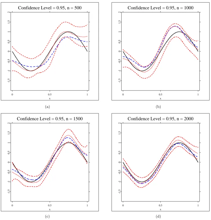
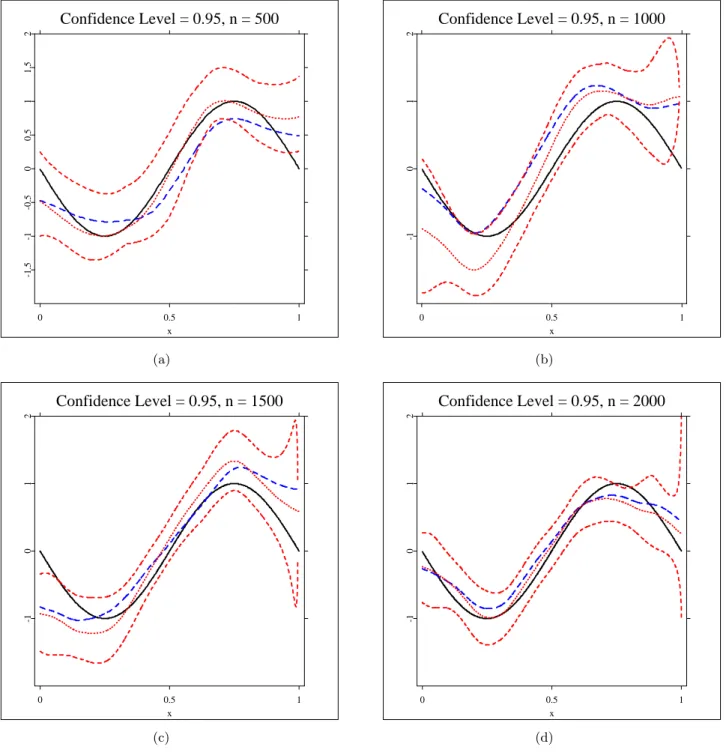
To have an impression of the actual function estimates, for𝑟 = 0, 𝑎= 0 and 𝑟 = 0.5, 𝑎= 0.5 with sample size 𝑛 = 500, 1000, 1500, 2000, we have plotted the SBK estimators and their 95% pointwise confidence intervals

(three dotted lines), oracle estimators (dashed lines) for the true functions 𝑚1(solid lines) in Figures2and3. The results are satisfactory and show that

the theory works in practice, and that performance improves with increasing sample size.

(Insert Figure2about here) (Insert Figure3about here)

6.3. Example 3. We have applied the estimation to the dataset comes from the credit reform database provided by the Research Data Center (RDC) of the Humboldt Universit¨at zu Berlin. After we exclude the miss-ing values, it contains financial information from 18610 solvent (𝑦= 0) and 1000 insolvent (𝑦 = 1) German companies. The time period ranges from 1997 to 2002 and in the case of the insolvent companies the information was gathered 2 years before the insolvency took place. For more details, see

H¨ardle et al.(2010). The financial ratios we use are showed in Table4.

(Insert Table4 about here)

In order to satisfy (A4), we make following transformation:𝑋𝑖𝛼 =𝐹𝑛𝛼(𝑍𝑖𝛼),

𝛼= 1, ...,8, where𝐹𝑛𝛼is the empirical cdf for the data {𝑋𝑖𝛼}𝑛_𝑖=1 . We

mea-sure the quality of the estimation by Accuracy Ratio (AR), which is the ratio of two areas. The first one is the area between the Cumulative Accu-racy Profile (CAP) curve and the diagonal line, and the second one is the area between the perfect model CAP curve and the diagonal. The second area is close to 1/2 in this example, so we have AR≈2∫₀1CAP (𝑥)𝑑𝑥−1.

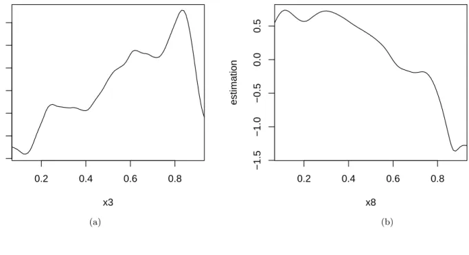
As a result, our model has the AR value 62.66%. We can also estimate the functions𝑚𝛼(𝑥) for𝑋𝛼. For example, if we are interested in the effects

of Ebit/Total Assets and log (Total Assets), we can obtain the estimations for𝑚3(𝑥) and𝑚8(𝑥), which are showed in Figure 4.

(Insert Figure4about here)

It is not a surprise that the estimation for𝑚8(𝑥) decreases as𝑥 value

in-creases. It means that a company with more Total Assets has smaller prob-ability of insolvent. While as 𝑥 value increases, the estimation for 𝑚3(𝑥)

increases for most part but decreases at the end. So generally, those compa-nies with higher Ebit/Total Assets ratio have more probability of insolvent. But it looks like that those companies with extremely high Ebit/Total Assets ratio have less probability of insolvent. It is an interesting topic to figure out the reason.

APPENDIX A: APPENDIX SECTION

A.1. Preliminaries. In the proofs that follow, we use “𝒰” and “𝒰” to

certain order.

LEMMA A.1. (Sunklodas (1984), Theorem 1) Let {𝜉_𝑖}𝑛_𝑖=1 be an 𝛼 -mixing sequence with E𝜉_𝑛 = 0. Denote 𝑑𝛿 = max1≤𝑖≤𝑛{E∣𝜉𝑖∣2+𝛿},0 <

𝛿 ≤ 1, 𝑆𝑛 = ∑𝑛_𝑖=1𝜉𝑖, 𝜎2𝑛 def= E𝑆𝑛2 ≥ 𝑐0𝑛 for some 𝑐0 ∈ (0,+∞). If

𝛼(𝑛)≤𝐾0exp (−𝜆0𝑛),𝜆0 >0,𝐾0 >0, then𝑐1 =𝑐1(𝐾0, 𝛿),𝑐2 =𝑐2(𝐾0, 𝛿)

exist such that

(A.1) Δ𝑛= sup 𝑧 P { 𝜎−_𝑛1𝑆𝑛< 𝑧}−Φ (𝑧)≤𝑐1_𝑐𝑑𝛿 0𝜎𝛿𝑛 { log(𝜎𝑛/𝑐1/2₀ ) /𝜆}1+𝛿

for any𝜆 with𝜆1≤𝜆≤𝜆2, where

𝜆1 =𝑐2 { log(𝜎𝑛/𝑐1/2₀ )}_𝑏 /𝑛, 𝑏 >2 (1 +𝛿)/𝛿;𝜆2 = 4 (2 +𝛿)𝛿−1log ( 𝜎𝑛/𝑐1/2₀ ) .

LEMMA A.2. (Bernstein’s inequality, Bosq (1998), Theorem 1.4) Let

{𝜉_𝑖} be a zero mean real valued process, and suppose that there exists 𝑐 > 0 such that for 𝑖 = 1,⋅ ⋅ ⋅ , 𝑛, 𝑘 ≥ 3, E∣𝜉_𝑖∣𝑘 ≤ 𝑐𝑘−2_𝑘!E𝜉2

𝑖 < +∞, 𝑚𝑟 =

max1≤𝑖≤𝑛∥𝜉𝑖∥𝑟, 𝑟≥2. Then for each 𝑛 >1, integer 𝑞∈[1, 𝑛/2], each 𝜀 >0

and𝑘≥3 P{∑𝑛 𝑖=1𝜉𝑖 > 𝑛𝜀}≤𝑎1exp ( −_25𝑚𝑞𝜀₂ 2 2+ 5𝑐𝜀 ) +𝑎2(𝑘)𝛼 ([ 𝑛 𝑞+ 1 ]) 2𝑘 2𝑘+1 where 𝑎1= 2𝑛_𝑞 + 2 ( 1 + 𝜀2 25𝑚2 2+ 5𝑐𝜀 ) , 𝑎2(𝑘) = 11𝑛 ( 1 +5𝑚2𝑘/(2𝑘+1)𝑘 𝜀 ) . Denote the theoretical inner product of𝑏𝐽 and 1 with respect to the𝛼-th

marginal density𝑓𝛼(𝑥𝛼) as 𝑐𝐽,𝛼 =⟨𝑏𝐽(𝑋𝛼),1⟩ =∫ 𝑏𝐽(𝑥𝛼)𝑓𝛼(𝑥𝛼)𝑑𝑥𝛼 and

define the centered B spline basis 𝑏𝐽,𝛼(𝑥𝛼) and the standardized B spline

basis𝐵𝐽,𝛼(𝑥𝛼) as 𝑏𝐽,𝛼(𝑥𝛼) =𝑏𝐽(𝑥𝛼)−_𝑐𝑐𝐽,𝛼 𝐽−1,𝛼𝑏𝐽−1(𝑥𝛼), 𝐵𝐽,𝛼(𝑥𝛼) = 𝑏𝐽,𝛼(𝑥𝛼) ∥𝑏𝐽,𝛼∥₂ ,1≤𝐽 ≤𝑁+ 1, so thatE𝐵𝐽,𝛼(𝑋𝛼) = 0,E𝐵𝐽,𝛼2 (𝑋𝛼) = 1.

LEMMAA.3. (Wang and Yang (2007), Theorem A.2) Under Assump-tions (A1)-(A5) and (A7), one has:

(i) Constants𝑐0(𝑓),𝐶0(𝑓),𝑐1(𝑓)and𝐶1(𝑓)exist depending on the marginal

densities 𝑓𝛼(𝑥𝛼),1≤𝛼≤𝑑, such that 𝑐0(𝑓)𝐻≤𝑐𝐽,𝛼≤𝐶0(𝑓)𝐻 and

(A.2) 𝑐1(𝑓)𝐻≤ ∥𝑏𝐽,𝛼∥2₂ ≤𝐶1(𝑓)𝐻.

(ii) uniformly for 𝐽, 𝐽′ _{= 1, ..., 𝑁+ 1} E{𝐵𝐽,𝛼(𝑋𝑖𝛼)𝐵𝐽′_,𝛼(𝑋_𝑖𝛼)}∼ ⎧   ⎨   ⎩ 1 𝐽′ _=𝐽 −1/3 ∣𝐽′_{−𝐽∣= 1} 1/6 ∣𝐽′_{−𝐽∣= 2} 0 ∣𝐽′_−𝐽∣>2 E𝐵𝐽,𝛼(𝑋𝑖𝛼)𝐵𝐽′_,𝛼(𝑋_𝑖𝛼)𝑘∼ { 𝐻1−𝑘 _∣𝐽′_{−𝐽∣ ≤2} 0 ∣𝐽′_−𝐽∣>2 , 𝑘≥1.

LEMMAA.4. (De Boor(2001), p.149) A constant𝐶∞>0 exists such that for any 𝑚 ∈ 𝐶1_{[0,1] with 𝑚}′ _{∈ Lip ([0,1], 𝐶∞), there is a function}

𝑔∈𝐺(0)𝑛 [0,1]such that ∥𝑔−𝑚∥_∞≤𝐶∞𝐻2.

LEMMAA.5. (Wang and Yang(2007), Lemma A.2) Constants𝑐0, 𝐶0 >

0 exist such that for any 𝝀= (𝜆0, 𝜆𝐽,𝛼)T_{1≤𝐽≤𝑁+1,1≤𝛼≤𝑑}∈ℝ1+𝑑(𝑁+1),

𝑐0 ( 𝜆2₀+∑2_𝐽,𝛼𝜆2_𝐽,𝛼)≤𝜆0+∑_𝐽,𝛼𝜆𝐽,𝛼𝐵𝐽,𝛼2 2 ≤𝐶0 ( 𝜆2₀+∑2_𝐽,𝛼𝜆2_𝐽,𝛼).

LEMMA A.6. (Xue and Yang (2006a), Lemma A.4) Under Assump-tions (A2), (A4) and (A6), as𝑛→ ∞, the uniform supremum of the rescaled difference between⟨𝑔1, 𝑔2⟩2,𝑛 and ⟨𝑔1, 𝑔2⟩2 is

𝐴𝑛= sup 𝑔1,𝑔2∈𝐺(0)𝑛 [0,1] ⟨𝑔1, 𝑔2⟩2,𝑛− ⟨𝑔1, 𝑔2⟩2 ∥𝑔1∥₂∥𝑔2∥₂ =𝒪𝑎.𝑠. ( log𝑛 𝑛1/2_𝐻1/2 ) .

A.2. Oracle smoothers.

LEMMA A.7. Under Assumptions (A1)-(A6), as 𝑛→ ∞,

sup 𝑥1∈[ℎ,1−ℎ] ˜𝑙′{𝑚1(𝑥1)} −bias1(𝑥1)ℎ2−𝑛−1∑𝑛_𝑖=1𝐾ℎ(𝑋𝑖1−𝑥1)𝜎(X𝑖)𝜀𝑖 =𝒪𝑎.𝑠. ( 𝑛−1/2ℎ1/2log𝑛)

Proof. According to (3.1) and (1.3), ˜𝑙′_{{𝑚1(𝑥1)}is} 𝑛−1∑𝑛_𝑖=1[𝑌𝑖−𝑏′{𝑚1(𝑥1) +𝑚1(X𝑖1)}]𝐾ℎ(𝑋𝑖1−𝑥1) (A.3) = 𝑛−1∑𝑛_𝑖=1[𝑏′{𝑚(X𝑖)} −𝑏′{𝑚1(𝑥1) +𝑚1(X𝑖1)}+𝜎(X𝑖)𝜀𝑖] 𝐾ℎ(𝑋𝑖1−𝑥1) Let𝜉_𝑖,𝑛=𝜉_𝑖,𝑛(𝑥1) =𝜉𝑖,𝑛,1+𝜉𝑖,𝑛,2 in which 𝜉_𝑖,𝑛,1(𝑥1) = [𝑏′{𝑚(X𝑖)} −𝑏′{𝑚1(𝑥1) +𝑚1(X𝑖1)}]𝐾ℎ(𝑋𝑖1−𝑥1) −E[[𝑏′{𝑚(X𝑖)} −𝑏′{𝑚1(𝑥1) +𝑚1(X𝑖1)}]𝐾ℎ(𝑋𝑖1−𝑥1)], (A.4) 𝜉_𝑖,𝑛,2=𝜉_𝑖,𝑛,2(𝑥1) =𝜎(X𝑖)𝜀𝑖𝐾ℎ(𝑋𝑖1−𝑥1).

Then according to (A.3), one can rewrite 𝑙∗′_{{𝑚1(𝑥1)} as}

𝑛−1∑𝑛_𝑖=1𝜉_𝑖,𝑛+E[𝑏′{𝑚(X𝑖)} −𝑏′{𝑚1(𝑥1) +𝑚1(X𝑖1)}]𝐾ℎ(𝑋𝑖1−𝑥1).

The deterministic term is

E[𝑏′{𝑚(X𝑖)} −𝑏′{𝑚1(𝑥1) +𝑚1(X𝑖1)}]𝐾ℎ(𝑋𝑖1−𝑥1) = ∫ 𝝌 [ 𝑏′{𝑚(u)} −𝑏′{𝑚1(𝑥1) +𝑚1(u1)}]ℎ−1𝐾 ( 𝑢1−𝑥1 ℎ ) 𝑓(u)𝑑u = ∫ 𝝌 [ 𝑏′′_{𝑚(𝑥 1,u1)} {𝑚1(𝑢1)−𝑚1(𝑥1)} +1 2𝑏′′′{𝑚(𝑥1,u1)} {𝑚1(𝑢1)−𝑚1(𝑥1)}2+𝒰 ( ℎ2)] ℎ−1𝐾 ( 𝑢1−𝑥1 ℎ ) 𝑓(𝑢1,u1)𝑑𝑢1𝑑u1+𝒰(ℎ2) = ∫ [0,1]𝑑−1 ∫ [−1,1] [ 𝑏′′{𝑚(𝑥1,u1)} { ℎ𝑣1𝑚′1(𝑥1) +(ℎ𝑣1) 2 2 𝑚′′1(𝑥1) +𝒰 ( ℎ2) } +1₂𝑏′′′{𝑚(𝑥1,u1)} { ℎ𝑣1𝑚′1(𝑥1) + (ℎ𝑣1)2𝑚′′1(𝑥1) +𝒰(ℎ2)} 2] 𝐾(𝑣1) { 𝑓(𝑥1,u1) +ℎ𝑣1∂𝑓(𝑥_∂𝑥1,u1) 1 +𝒰 ( ℎ2)}_𝑑𝑣 1𝑑u1+𝒰(ℎ2) which equals ℎ2 ∫ [−1,1]𝑣 2 1𝐾(𝑣1)𝑑𝑣1 { 𝑚′′ 1(𝑥1)𝑓1(𝑥1) 2 ∫ [0,1]𝑑−1𝑏 ′′_{𝑚(𝑥 1,u1)}𝑓(u∣𝑥1)𝑑u1 +𝑚′₁(𝑥1) ∫ [0,1]𝑑−1𝑏 ′′_{𝑚(𝑥 1,u1)}∂𝑓(𝑥_∂𝑥1,u1) 1 𝑑u1 } +𝒰(ℎ2).

= ℎ2𝜇₂(𝐾){𝑚′′₁(𝑥1)𝑓(𝑥1)E[𝑏′′{𝑚(X)} ∣𝑋1 =𝑥1] +𝑚′₁(𝑥1)_∂𝑥∂ 1 [ 𝑓(𝑥1)E[𝑏′′{𝑚(X)} ∣𝑋1 =𝑥1]] −{𝑚′ 1(𝑥1)}2𝑓(𝑥1)E[𝑏′′′{𝑚(X)} ∣𝑋1 =𝑥1]}+𝒰(ℎ2) = bias1(𝑥1)ℎ2+𝒰(ℎ2).

Using the above

E𝜉2 𝑖,𝑛,1 = ℎ−2 ∫ [0,1]𝑑 [ 𝑏′_{{𝑚(u)} −𝑏}′_{𝑚 1(𝑥1) +𝑚1(u1)}]2 𝐾 ( 𝑢1−𝑥1 ℎ )₂ 𝑓(u)𝑑u+𝒰(ℎ4) = ℎ−1 ∫ [0,1]𝑑−1 ∫ [−1,1] [ 𝑏′{𝑚(𝑥1+ℎ𝑣1,u1)} −𝑏′{𝑚1(𝑥1) +𝑚1(u1)}]2 𝐾(𝑣1)2𝑓(𝑥1+ℎ𝑣1,u1)𝑑𝑣1𝑑u1+𝒰(ℎ4) = ℎ−1 ∫ [0,1]𝑑−1 ∫ [−1,1] [ 𝑏′′{𝑚(𝑥1,u−1)}{ℎ𝑣1𝑚′1(𝑥1) +𝒰(ℎ2)}]2 𝐾(𝑣1)2{𝑓(𝑥1,u1) +𝒰(ℎ)}𝑑𝑣1𝑑u1+𝒰(ℎ4)=𝒰(ℎ).

Note that sup_𝑥1∣𝑏′_{{𝑚(X𝑖)} −𝑏}′_{{𝑚1(𝑥1) +𝑚1(X𝑖1)}∣ ≤𝐶𝑏ℎ whenever}

𝐾ℎ(𝑋𝑖1−𝑥1)∕= 0, hence E𝜉𝑖,𝑛,1𝑘 ≤(2𝐶𝑏ℎ)𝑘−2E𝜉2𝑖,𝑛,1 so applying Lemma

A.2implies that sup_{𝑥1∈[ℎ,1−ℎ]}𝑛−1∑𝑛

𝑖=1𝜉𝑖,𝑛,1=𝒪𝑎.𝑠.{ℎ1/2𝑛−1/2log𝑛}. □

LEMMA A.8. Under Assumptions (A2), (A4)-(A6), as 𝑛→ ∞

sup 𝑥1∈[ℎ,1−ℎ] ˜𝑙′′_(𝑚 1(𝑥1)) +𝐷1(𝑥1)=𝒪𝑎.𝑠. ( log𝑛/√𝑛ℎ), where 𝐷1(𝑥1) is defined in (3.3).

Proof. SeeLiu et al.(2011). □

LEMMA A.9. Under Assumptions (A1) to (A3), (A5) and (A7), a constant 𝐶 exists such that, as𝑛→ ∞

sup

𝑥1∈[ℎ,1−ℎ] _Cov(

Proof.According to Davydov’s inequality, for_𝑝1+1_𝑞+_𝑟1 = 1,Cov(𝜉_𝑖,𝑛, 𝜉_𝑗,𝑛) is bounded by

𝐶2{2𝛼(𝑗−𝑖)}1/𝑝𝜉𝑖,𝑛,1+𝜉𝑖,𝑛,2_𝑞𝜉𝑗,𝑛,1+𝜉𝑗,𝑛,2_𝑟

≤ 𝐶2{2𝛼(𝑗−𝑖)}1/𝑝(𝜉𝑖,𝑛,1_𝑞+𝜉𝑖,𝑛,2_𝑞) (𝜉𝑗,𝑛,1_𝑟+𝜉𝑗,𝑛,2_𝑟 )

Let 𝑞 =𝑟 = 2 +𝜂, 𝑝 = 1 + 2/𝜂, where 𝜂 takes value in the (A3), then one has𝜉_{𝑖,𝑛,1𝑞} =𝒰(ℎ−2+1𝜂)and 𝜉

𝑖,𝑛,1_𝑞 =𝒰 (

ℎ−1+2+𝜂𝜂).Cov(𝜉

𝑖,𝑛,𝑙′, 𝜉_{𝑗,𝑛,𝑙}′′)≤

𝐶ℎ−1+2+𝜂𝜂𝛼(𝑗−𝑖)2+𝜂𝜂 for some constant𝐶. □

Proof of Theorem 1 and Theorem 2. The Mean Value Theorem ensures the existence of a ¯𝑚1(𝑥1) between ˜𝑚K,1(𝑥1) and𝑚1(𝑥1) such that

˜

𝑙′{𝑚˜_K,1(𝑥1)} −˜𝑙′{𝑚1(𝑥1)}= ˜𝑙′′{𝑚˜1(𝑥1)} {𝑚˜K,1(𝑥1)−𝑚1(𝑥1)}

Note that ˜𝑙′_{{𝑚˜K,1(𝑥1)}= 0 yielding}

(A.5) 𝑚˜K,1(𝑥1)−𝑚1(𝑥1) =−

˜

𝑙′_{(𝑚1(𝑥1))}

˜

𝑙′′_{( ¯𝑚1(𝑥1))}.

LemmaA.8, Lemma A.7and (A.5) then imply Theorem1.

Let 𝑆𝑛 = 𝑆𝑛(𝑥1) = ∑𝑛_𝑖=1𝜉𝑖,𝑛, where 𝜉𝑖,𝑛 is defined as (A.4). Note that E𝑆𝑛= 0 and ˜𝑙′{𝑚1(𝑥1)}=𝑆𝑛/𝑛+𝑏(𝑥1)ℎ2+𝒰(ℎ2). 𝛾(𝑘) =𝛾(𝑘, 𝑥1) =Cov(𝜉𝑖,𝑛, 𝜉𝑖+𝑘,𝑛 ) 𝜎2_𝑛 = E𝑆_𝑛2 =Var(𝑆𝑛) =Var(∑𝑛_𝑖=1𝜉𝑖,𝑛 ) = ∑𝑛_𝑖=1Var(𝜉_𝑖,𝑛)+∑𝑛_𝑖∕=𝑗Cov(𝜉_𝑖,𝑛, 𝜉_𝑗,𝑛) = 𝑛Var(𝜉_𝑖,𝑛)+𝑛∑_{1≤∣𝑘∣≤𝑛−1} ( 1−∣_𝑛𝑘∣ ) 𝛾(𝑘) = 𝑛Var(𝜉_𝑖,𝑛)+𝑛𝐴𝑛, where Var(𝜉_𝑖,𝑛)=ℎ−1_𝑓 1(𝑥1)E{𝜎2(X)∣𝑋1 =𝑥1}∥𝐾∥22+𝒰 ( ℎ4)_.

According to LemmaA.9, one has

Hence ∣𝐴𝑛∣ = ∑1≤∣𝑙∣≤𝑛−1𝛾(𝑘) ≤ ∑_{1≤∣𝑙∣≤𝑛−1} ( 1−∣_𝑛𝑘∣ ) ℎ−1+2+𝜂𝜂{𝐾₀exp (−𝜆₀𝑘)}2+𝜂𝜂 ≤ 𝐾0ℎ− 1+𝜂 2+𝜂 ∑ 1≤∣𝑙∣≤𝑛−1exp{−𝜆0𝑘𝜂/(2 +𝜂)},

so a constant𝐶1exists such that𝐴𝑛≤𝐶1ℎ− 1+𝜂

2+𝜂, and therefore𝐴_𝑛/Var(𝜉_𝑖,𝑛)→

0 as 𝑛 → ∞. Since 𝜎2

𝑛 ∼ 𝑛Var (

𝜉_𝑖,𝑛) ≥ 𝑐0𝑛 when 𝑛 is large, according to

(A.1) in LemmaA.1, constants𝑐1 and𝑐2 exist such that for some 0< 𝜂≤1

(A.6) Δ𝑛= sup 𝑧 P { 𝜎−1 𝑛 𝑆𝑛< 𝑧}−Φ (𝑧)≤𝑐1_𝑐𝑑𝜂 0𝜎𝜂𝑛 { log(𝜎𝑛/𝑐1/20 ) /𝜆}1+𝜂 for any𝜆with𝜆1 ≤𝜆≤𝜆2, where

𝜆1 =𝑐2 { log(𝜎𝑛/𝑐1/2₀ )}_𝑏 /𝑛, 𝑏 >2 (1 +𝜂)/𝜂;𝜆2= 4 (2 +𝜂)𝜂−1log ( 𝜎𝑛/𝑐1/2₀ ) . For 𝜂 in (A3), set 𝜆= 4 (2 +𝜂)𝜂−1_log(_𝜎

𝑛/𝑐1/20 )

, then by (A6), the 𝑑𝜂 in

(A.6) is 𝑑𝜂 = max_{1≤𝑖≤𝑛}(E[𝑏′{𝑚(X𝑖)} −𝑏′{𝑚1(𝑥1) +𝑚1(X𝑖1)}+𝜎(X𝑖)𝜀𝑖] 𝐾ℎ(𝑋𝑖1−𝑥1)∣2+𝜂 ) = max 1≤𝑖≤𝑛 { E∣𝐶𝑏ℎ+𝜎(X𝑖)𝜀𝑖∣2+𝜂∣𝐾ℎ(𝑋𝑖1−𝑥1)∣2+𝜂 } ≤ 𝐶𝐶𝛿𝐶𝜂{E∣𝐾ℎ(𝑋1−𝑥1)∣2+𝜂}=𝒪 { ℎ−(1+𝜂)}, i.e., Δ𝑛=𝒪{ℎ−(1+𝜂)/𝜎𝜂𝑛}=𝒪{𝑛(1+𝜂/2)/5−𝜂/2}=𝒪(𝑛1/5−2𝜂/5)→0 when 1/2< 𝜂≤1. So𝑆𝑛/𝜎𝑛→ℒ 𝑁(0,1), then 𝑛[𝑙∗′{𝑚1(𝑥1)} −bias1(𝑥1)ℎ2]/ √ 𝑛ℎ−1_𝑣2 1(𝑥1)→ℒ 𝑁(0,1), where𝑣2

1(𝑥1) is defined in (3.5). According to Theorem1, one has as𝑛→ ∞,

sup_{𝑥1∈[ℎ,1−ℎ]}˜𝑙′′_{𝑚

1(𝑥1)} −˜𝑙′′{𝑚¯1(𝑥1)}→0 because

sup_{𝑥1∈[ℎ,1−ℎ]}∣𝑚1(𝑥1)−𝑚¯1(𝑥1)∣ →0. Then according to Slutsky’s theorem: √

where𝐷1(𝑥1) is defined in (3.3). □

Proof of Theorem 3. According to the Mean Value Theorem, a con-stant ¯𝑐between𝑐and ˜𝑐exists such that (˜𝑐−𝑐) ˜𝑙′′

𝑐(¯𝑐) = ˜𝑙′𝑐(˜𝑐)−𝑙˜′𝑐(𝑐) =−˜𝑙𝑐′(𝑐),

where −˜𝑙′′

𝑐 (¯𝑐) = 𝑛−1∑𝑛𝑖=1𝑏′′{𝑐¯+𝑚𝑐(X𝑖)} > 𝑐𝑏 > 0 according to (A2)

and where 𝑚𝑐(X) = ∑𝑑_𝛼=1𝑚𝛼(𝑋𝛼) and then the infeasible estimator is

˜

𝑐= argmax_𝑎∈𝐴˜𝑙𝑐(𝑎).Clearly, ˜𝑙′𝑐(˜𝑐) = 0 and

˜ 𝑙′_𝑐(𝑐) = 𝑛−1∑𝑛_𝑖=1[𝑌𝑖−𝑏′{𝑐+𝑚𝑐(X𝑖)}] = 𝑛−1∑𝑛 𝑖=1𝜎(X𝑖)𝜀𝑖 =𝒪𝑎.𝑠 ( 𝑛−1/2_log𝑛)

by Bernstein’s Inequality. Similarly, ˜𝑙′′

𝑐(𝑐) = −𝑛−1∑𝑛𝑖=1𝑏′′{𝑐+𝑚𝑐(X𝑖)}

converges to −E𝑏′′_{{𝑚(X)} almost surely at the rate of𝑛}−1/2_{log𝑛. These}

imply that∣˜𝑐−𝑐∣=𝒪𝑎.𝑠.(𝑛−1/2log𝑛) and plugging it into

(˜𝑐−𝑐) =−˜𝑙′

𝑐(𝑐)/˜𝑙′′𝑐(¯𝑐), Theorem3 is proved. □

A.3. Spline backfitted kernel estimators. In this section, we present the proof of Theorem 4. We write any 𝑔 ∈ 𝐺0

𝑛 as 𝑔 = 𝝀TB(X𝑖) with

vec-tor 𝝀= (𝜆0, 𝜆𝐽,𝛼)T_{1≤𝐽≤𝑁+1,1≤𝛼≤𝑑} ∈ 𝑅𝑁𝑑 where 𝑁𝑑 = (𝑁 + 1)𝑑+ 1 is the

dimension of the additive spline space𝐺0 𝑛, and

B(x) ={1, 𝐵1,1(𝑥1), ..., 𝐵𝑁+1,𝑑(𝑥𝑑)}T,

its standardized basis. We denote with a slight abuse of notation ˆ

𝐿(𝑔) = ˆ𝐿(𝝀) = 𝑛−1∑𝑛 𝑖=1

[

𝑌𝑖𝝀TB(X𝑖)−𝑏{𝝀TB(X𝑖)}], which yields the

gradient and Hessian formulae

∇𝐿ˆ(𝝀) = 𝑛−1∑_𝑖=1𝑛 [𝑌𝑖B(X𝑖)−𝑏′ { 𝝀TB(X𝑖) } B(X𝑖) ] , ∇2_{𝐿ˆ(𝝀) = −𝑛}−1∑𝑛 𝑖=1𝑏′′ { 𝝀T_B(X 𝑖) } B(X𝑖)B(X𝑖)T.

The multivariate function𝑚(x) is estimated by an additive spline func-tion ˆ 𝑚(x) = ˆ𝑚0+∑𝑑𝛼=1𝑚ˆ𝛼(𝑥𝛼) =𝝀ˆTB(x), ˆ 𝝀 = (𝜆ˆ0,𝜆ˆ𝐽,𝛼 )_T 1≤𝛼≤𝑑 1≤𝐽≤𝑁+1 = argmax𝝀 ˆ 𝐿(𝝀).

Lemma 14 of Stone (1986) ensures that with probability approaching 1, ˆ𝝀

exists uniquely and that ∇𝐿ˆ(𝝀ˆ)=0. In addition, Lemma A.4 and (A1) provide a vector¯𝝀and an additive spline function ¯𝑚 such that

(A.7) 𝑚¯ (x) =𝝀¯TB(x),∥𝑚¯ −𝑚∥_∞≤𝐶∞𝐻2.

LEMMA A.10. Under Assumptions (A1)-(A5) and (A7), as 𝑛→ ∞ ∇𝐿ˆ(𝝀¯) = 𝒪𝑎.𝑠. ( 𝐻2+𝑛−1/2log𝑛), ∇𝐿ˆ(¯𝝀) = 𝒪𝑎.𝑠. ( 𝐻3/2_+𝐻−1/2_𝑛−1/2_log𝑛)_. Proof. ∇𝐿ˆ(𝝀¯) = 𝑛−1∑𝑛_𝑖=1[𝑌𝑖B(X𝑖)−𝑏′{¯𝝀TB(X𝑖)}B(X𝑖)] = 𝑛−1∑𝑛_𝑖=1[𝑏′{𝑚(X𝑖)} −𝑏′{𝑚¯ (X𝑖)}+𝜎(X𝑖)𝜀𝑖]B(X𝑖)

The first element of the above vector is

1 𝑛

∑_𝑛

𝑖=1[[𝑏′{𝑚(X𝑖)} −𝑏′{𝑚¯ (X𝑖)}] +𝜎(X𝑖)𝜀𝑖], which is𝒪𝑎.𝑠.(𝐻2+𝑛−1/2log𝑛)

according to LemmasA.4 and A.2. The other elements can be written as 𝑛−1∑𝑛_𝑖=1[𝜉_{𝑖,𝐽,𝛼,𝑛}+E[𝑏′{𝑚(𝑋𝑖𝛼)} −𝑏′{𝑚¯ (𝑋𝑖𝛼)}] 𝐵𝐽,𝛼(𝑋𝑖𝛼) +𝜎(X𝑖)𝜀𝑖𝐵𝐽,𝛼(𝑋𝑖𝛼)], where 𝜉_{𝑖,𝐽,𝛼,𝑛} = [𝑏′_{𝑚(𝑋 𝑖𝛼)} −𝑏′{𝑚¯ (𝑋𝑖𝛼)}]𝐵𝐽,𝛼(𝑋𝑖𝛼) −E[[𝑏′_{𝑚(𝑋 𝑖𝛼)} −𝑏′{𝑚¯ (𝑋𝑖𝛼)}]𝐵𝐽,𝛼(𝑋𝑖𝛼)].

According to (A.2) and (A.7), one has

_E[ 𝑏′{𝑚(𝑋𝑖𝛼)} −𝑏′{𝑚¯ (𝑋𝑖𝛼)}]𝐵𝐽,𝛼(𝑋𝑖𝛼) ≤ E𝑏′{𝑚(𝑋𝑖𝛼)} −𝑏′{𝑚¯ (𝑋𝑖𝛼)}∣𝑏𝐽,𝛼_∥𝑏(𝑋𝑖𝛼)∣ 𝐽,𝛼∥₂ ≤ 𝑐∥𝑚−𝑚¯∥_∞ max 1≤𝐽≤𝑁+1 1≤𝛼≤𝑑 ∥𝑏𝐽,𝛼∥−₂1_1≤max_{𝐽≤𝑁+1} 1≤𝛼≤𝑑 E∣𝑏𝐽,𝛼(𝑋𝑖𝛼)∣ = 𝒪(𝐻2_×𝐻−1/2_×𝐻)_=𝒪(_𝐻5/2)_,

for some constant𝑐and likewise for any 𝑘≥2

E𝑏′{𝑚(𝑋𝑖𝛼)} −𝑏′{𝑚¯ (𝑋𝑖𝛼)}𝑘∣𝐵𝐽,𝛼(𝑋𝑖𝛼)∣𝑘 ≤ 𝑐𝑘−2_{∥𝑚−𝑚¯∥}𝑘−2 ∞ _1≤max_{𝐽≤𝑁+1} 1≤𝛼≤𝑑 ∥𝑏𝐽,𝛼∥−2(𝑘−2)_1≤max_{𝐽≤𝑁+1} 1≤𝛼≤𝑑 E𝑏𝑘−2 𝐽,𝛼 (𝑋𝑖𝛼) ×E𝑏′_{𝑚(𝑋 𝑖𝛼)} −𝑏′{𝑚¯ (𝑋𝑖𝛼)}2 𝑏 2 𝐽,𝛼(𝑋𝑖𝛼) ∥𝑏𝐽,𝛼∥2₂ ≤ (𝑐𝐻5/2)𝑘−2_E𝑏′_{𝑚(𝑋 𝑖𝛼)} −𝑏′{𝑚¯ (𝑋𝑖𝛼)}2 𝑏 2 𝐽,𝛼(𝑋𝑖𝛼) ∥𝑏𝐽,𝛼∥2₂