Real-Time Simulation of Indoor Air Flow using the Lattice Boltzmann Method on Graphics Processing Unit

R E A L - T I M E S I M U L AT I O N O F I N D O O R A I R F L O W U S I N G T H E L AT T I C E B O LT Z M A N N M E T H O D

O N G R A P H I C S P R O C E S S I N G U N I T n i c o l a s d e l b o s c

Submitted in accordance with the requirements for the degree of Doctor of Philosophy

School of Mechanical Engineering Faculty of Engineering

The candidate confirms that the work submitted is his own and that appropriate credit has been given where reference has been made to the work of others.

This copy has been supplied on the understanding that it is copyright material and that no quotation from the thesis may be published without proper

acknowledgement.

The right of Nicolas Delbosc to be identified as Author of this work has been asserted by him in accordance with the Copyright, Designs and Patents Act1988.

A C K N O W L E D G M E N T S

I would like to thank my supervisors, Dr. J.L. Summers, and Dr. A.I. Khan, for their continued support and invaluable discussions throughout my time as a PhD student at the University of Leeds.

Furthermore, I would like to extend my gratification to my fellow PhD students who helped make my time at the School of Mechanical Engineering both a rewarding and enjoyable experience.

Finally, I would like to thank NVIDIA for donating two K40 GPUs through the hardware donation program.

A B S T R A C T

This thesis investigates the usability of the lattice Boltzmann method (LBM) for the simulation of indoor air flows in real-time. It describes the work undertaken during the three years of a Ph.D. study in the School of Mechanical Engineering at the University of Leeds, Eng-land.

Real-time fluid simulation, i.e. the ability to simulate a virtual sys-tem as fast as the real syssys-tem would evolve, can benefit to many engi-neering application such as the optimisation of the ventilation system design in data centres or the simulation of pollutant transport in hos-pitals. And although real-time fluid simulation is an active field of re-search in computer graphics, these are generally focused on creating visually appealing animation rather than aiming for physical accu-racy. The approach taken for this thesis is different as it starts from a physics based model, the lattice Boltzmann method, and takes advan-tage of the computational power of a graphics processing unit (GPU) to achieve real-time compute capability while maintaining good phys-ical accuracy.

The lattice Boltzmann method is reviewed and detailed references are given a variety of models. Particular attention is given to turbu-lence modelling using the Smagorinsky model in LBM for the simu-lation of high Reynolds number flow and the coupling of two LBM simulations to simulate thermal flows under the Boussinesq approxi-mation.

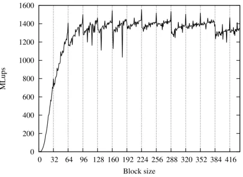
A detailed analysis of the implementation of the LBM on GPU is conducted. A special attention is given to the optimisation of the al-gorithm, and the program kernel is shown to achieve a performance of up to 1.5 billion lattice node updates per second, which is found to be sufficient for coarse real-time simulations. Additionally, a re-view of the real-time visualisation integrated within the program is presented and some of the techniques for automated code generation are introduced.

The resulting software is validated against benchmark flows, using their analytical solutions whenever possible, or against other simu-lation results obtained using accepted method from classical compu-tational fluid dynamics (CFD) either as published in the literature or simulated in-house. The LBM is shown to resolve the flow with similar accuracy and in less time.

P U B L I C AT I O N S & TA L K S

Some ideas and figures have appeared previously in the following publications and conference talks:

p u b l i c at i o n s

• A.I. Khan, N. Delbosc, J.L. Summers, C.J. Noakes.

Real-time flow simulation of indoor environments using the Lattice Boltzmann Method.

Journal of Building Simulation. August2015, Volume8, Issue4, Pages405–414.

http://dx.doi.org/10.1007/s12273-015-0232-9

• N. Delbosc, J.L. Summers, A.I. Khan, N. Kapur, C.J. Noakes. Optimised Implementation of the Lattice Boltzmann Method on a Graphics Processing Unit Towards Real-Time Fluid Simulation. Computer & Mathematics with Applications. February 2014, Volume67, Issue2, Pages462–475.

http://dx.doi.org/10.1016/j.camwa.2013.10.002

c o n f e r e n c e ta l k s

• N. Delbosc, K.H. Luo, J.L. Summers.

Lattice Boltzmann Method for Turbulence : Real-Time Simulation and Big Data Processing.

Whither Turbulence and Big Data for the21st century, Corsica, France, April20–24,2015.

• N. Delbosc, A.I. Khan, J.L. Summers.

Saving Energy in Data Centers Using Real-Time Simulation.

GPU Technology Conference (GTC 2015), San Jose, California, USA, March16–20,2015.

• N. Delbosc.

Real-Time Fluid Simulation.

Villanova University, Philadelphia, USA, March 10, 2015. (in-vited talk)

• N. Delbosc, J. Summers, A. Khan, C. Noakes.

Real-time simulation and visualisation of air flow in datacenters and hospitals.

23rd International Conference on Discrete Simulation of Fluid Dynamics (DSFD2014), Paris, France, July28 – August1,2014.

• N. Delbosc, GdeBoer, J.L. Summers.

Managing data centres with the aid of real-time airflow simulations. Datacentre Transformation Conference (DTC2014), Manchester, U.K., July8,2014

• N. Delbosc, A.I. Khan, J.L. Summers, C.J. Noakes.

Real-time Simulations and Visualisation of Air Flow in Datacenters and Hospitals.

GPU Technology Conference (GTC 2014), San Jose, California, USA, March24–27,2014.

• N. Delbosc, J.L. Summers, A.I. Khan.

Real-time Simulation of Air Flow in Datacenters and Hospitals. International Conference for Mesoscopic Methods in Engineer-ing and Science (ICMMES2013), Oxford, U.K., July22–26,2013. • N. Delbosc, J.L. Summers, A.I. Khan.

Real-Time Indoor Air Flow Simulation Using Lattice Boltzmann Method on GPU.

International Conference for Mesoscopic Methods in Engineer-ing and Science (ICMMES 2012), Taipei, Taiwan, July 23–27, 2012.

• N. Delbosc, J.L. Summers.

Nanofluid Simulation Using the Lattice Boltzmann Method on Graph-ics Processing Unit.

Workshop on Nanomaths. Centre de Recerca Matemàtica (CRM), Bellaterra, Barcelona, Spain, July11-13,2012.

C O N T E N T S

1 i n t r o d u c t i o n 1

1.1 Background and Motivations . . . 1

1.2 Computational fluid dynamics (CFD) . . . 2

1.2.1 Numerical Methods for CFD . . . 4

1.2.2 Thermal Flows . . . 6

1.2.3 Multiphase Flows . . . 6

1.2.4 Turbulence Modelling . . . 7

1.2.5 Commercial CFD Software. . . 9

1.3 Real-Time Fluid Simulation . . . 10

1.4 Lattice Boltzmann Method (LBM) . . . 14

1.5 Graphics Processing Unit (GPU) . . . 17

1.6 Objectives of the Thesis . . . 18

1.7 Thesis Outline . . . 19

2 t h e l at t i c e b o lt z m a n n m e t h o d 21 2.1 Introduction . . . 21

2.1.1 Historical background . . . 21

2.1.2 Kinetic Theory . . . 22

2.1.3 The Boltzmann Equation . . . 23

2.1.4 The BGK Approximation . . . 24

2.1.5 Multiple Relaxation Times . . . 25

2.2 General Framework of the LBM . . . 26

2.2.1 Space and Time Discretisation . . . 27

2.2.2 Algorithm . . . 28

2.3 LBM for multi-physics applications . . . 29

2.3.1 Standard LBM Model . . . 30

2.3.2 Incompressible Model . . . 31

2.3.3 LBM for Compressible Flows . . . 33

2.3.4 Multiphase and Multicomponent Models . . . . 33

2.3.5 Thermal Models . . . 39

2.3.6 Fluid-Structure Interaction . . . 43

2.4 Alternative Models . . . 45

2.4.1 Entropic LBM . . . 45

2.4.2 Cascaded LBM . . . 47

2.4.3 Link-Wise Artificial Compressibility Method . . 48

2.4.4 Further Reading . . . 49

2.5 Turbulence modelling in LBM . . . 50

2.5.1 Large Eddy Simulation . . . 50

2.5.2 RANS Based Models . . . 52

2.5.3 Further Reading . . . 52

2.6 LBM with Non-Uniform Grids . . . 53

2.7 Summary . . . 54

3.1 Program Framework . . . 58 3.1.1 Initialisation Step . . . 58 3.1.2 Streaming Step . . . 58 3.1.3 Collision Step . . . 59 3.1.4 Boundary Step . . . 61 3.2 Boundary Conditions . . . 62 3.2.1 Periodic . . . 62 3.2.2 Force Equilibrium . . . 63 3.2.3 Bounce-Back . . . 63 3.2.4 Free Slip . . . 65 3.2.5 Zou-He . . . 66 3.2.6 Ho-Cheng-Lin . . . 67 3.2.7 Interpolated Bounce-Back . . . 68

3.2.8 Immersed Boundary Method . . . 70

3.2.9 Further Reading . . . 72

4 o p t i m i s e d i m p l e m e n tat i o n o n g p u 73 4.1 A Brief History of GPU . . . 73

4.2 Introduction to GPU programming . . . 75

4.2.1 GPU programming methodology . . . 75

4.2.2 Differences between CPU and GPU . . . 76

4.2.3 SIMD programming philosophy . . . 77

4.2.4 Code sample . . . 78

4.3 Implementation of the LBM on GPU . . . 79

4.4 Optimisation of the LBM on GPU . . . 80

4.4.1 Minimise memory access . . . 81

4.4.2 Increase data coalescence . . . 82

4.4.3 The streaming issue . . . 86

4.4.4 Branch Divergence . . . 87

4.4.5 Other optimisations . . . 89

4.5 Real-time interactive visualisation . . . 90

4.6 Multi-GPU programming . . . 91

4.7 GPU code generation . . . 93

4.8 Summary . . . 96

5 c o m p u tat i o na l p e r f o r m a n c e 97 5.1 Performance Study . . . 97

5.1.1 On measuring performances . . . 97

5.1.2 Single GPU performances . . . 98

5.1.3 Multi-GPU performances . . . 100

5.1.4 Maximum performance . . . 101

5.1.5 Performance of other models . . . 103

5.1.6 Effect of the streaming model . . . 103

5.1.7 The issue of branch divergence . . . 104

5.2 Optimisation tricks and tweaks . . . 105

5.2.1 Using the NVIDIA Visual Profiler . . . 105

5.2.2 Tweaking for the best performance . . . 109

5.2.4 GPU boost . . . 113 5.3 Real-Time Capability . . . 114 5.4 Summary . . . 116 6 va l i d at i o n 117 6.1 2D Poiseuille Flow . . . 117 6.2 Lid-driven cavity . . . 121 6.2.1 Problem description . . . 121 6.2.2 Two-dimensional results . . . 122 6.2.3 Three-dimensional results . . . 133

6.3 Thermal diffusion in a square cavity . . . 136

6.3.1 Problem description. . . 136

6.3.2 Effect of the choice of boundary condition . . . 137

6.3.3 Effect of the initial temperature. . . 138

6.3.4 Effect of the relaxation time . . . 139

6.3.5 Effect of the lattice resolution . . . 139

6.3.6 Conclusion . . . 140

6.4 Thermal advection in a channel . . . 140

6.4.1 Problem description . . . 140

6.4.2 Analytical solution . . . 141

6.4.3 Results and Discussion . . . 142

6.4.4 Conclusion . . . 143

6.5 Natural convection in a square cavity . . . 144

6.5.1 Methodology . . . 146

6.5.2 Effect of the Rayleigh number. . . 147

6.5.3 Effect of the resolution. . . 149

6.5.4 Effect of the forcing scheme . . . 150

6.6 Summary . . . 151 7 a p p l i c at i o n t o i n d o o r a i r f l o w s 153 7.1 Introduction . . . 153 7.2 Ventilation Chamber . . . 154 7.2.1 Problem Description . . . 155 7.2.2 Results . . . 157 7.2.3 Conclusion . . . 160 7.3 Data centre . . . 163 7.3.1 Problem Description . . . 163 7.3.2 Results . . . 168 7.3.3 Conclusion . . . 170 7.4 Hospital Room . . . 171 7.5 Summary . . . 174 8 o t h e r a p p l i c at i o n s 175 8.1 Introduction . . . 175 8.2 Multiphase Flows . . . 175 8.2.1 Droplet Impingement . . . 176

8.2.2 Water in Diesel Filtration . . . 179

8.3 Drag and lift on cylinder . . . 181

8.5 MRT and Cascaded parameter search optimisation . . 186 8.6 Summary . . . 192 9 c o n c l u s i o n s 193 9.1 Summary of Results . . . 193 9.2 Future Work . . . 195 a n o d e d e s c r i p t i o n s 197 a.1 D2Q9 . . . 197 a.2 D3Q19 . . . 198 b u n i t c o n v e r s i o n 199 c f a s t f l u i d d y na m i c s 203 c.1 History . . . 203 c.2 Theory . . . 203

c.2.1 The Navier-Stokes equation . . . 203

c.2.2 Helmholtz-Hodge decomposition theorem . . . 204

c.2.3 Chorin’s projection algorithm . . . 204

c.3 JosStam’s algorithm . . . 205

c.3.1 Summary of the method . . . 205

c.3.2 Advection . . . 206 c.3.3 Diffusion . . . 206 c.3.4 Force . . . 208 c.3.5 Projection . . . 208 c.4 Implementation . . . 208 c.5 Numerical Experiment . . . 209 c.6 Summary . . . 209 d i n t r o d u c t i o n t o g p u p r o g r a m m i n g i n c u d a 211 d.1 Architecture . . . 211

d.1.1 CUDA Thread Organization . . . 211

d.1.2 Memory model . . . 213

d.2 Programing Model . . . 214

d.2.1 Threads and Kernels . . . 215

d.2.2 Memory Management . . . 216

d.3 Execution Model . . . 218

1

1.1 b a c k g r o u n d a n d m o t i vat i o n s

Simulations are at the core of all scientific modelling.

The wordsimulationcomes from the Latin adjectivesimilis,meaning similar. In this context, simulatinga physical system can be regarded as making something similar to it, whether it is building a scaled ex-periment or solving the equations that model its behaviour. This can be done for a variety of reasons: to gain a better understanding of its functioning, to study alternative conditions, and more... but in general, the goal is to improve a particular aspect of the system. The recourse to simulations can become necessary when the real system cannot be directly accessed or modified or when its manufacturing cost would be too high.

Often, computer simulations are used to study a model, and they have become essential in the modelling of many natural systems in physics, chemistry and biology, but also human systems in economics or social science. Numerical simulations are nowadays an integral part of engineering, as the equations that describe the motion of an aircraft or the stiffness of a bridge are often too complex to be solved without the help of computers.

But despite the growth in both speed and memory of computers over the last decades, computer simulations are still regarded as a complicated task. And engineering problems commonly require large simulations that run for many hours on a dedicated cluster of comput-ers, called a supercomputer. In particular, the domain ofcomputational fluid dynamics (CFD, see section1.2), that is the numerical simulation

of fluid flows, has become associated with long running programs consuming a lot of computational resources. This is because CFD usually involves complex time dependant non-linear partial differen-tial equations that are difficult to solve, even with the best computers. The goal of this thesis is to develop new simulation tools, based on novel numerical models and novel computer architectures, that will allow for a real-time and interactive simulation of various fluid flow problems applicable to engineering, and in particular indoor airflows. The study, prediction and control of indoor airflows is of prime im-portance in engineering and sprouts to many fields of applications, from air conditioning for human comfort to thermal management for equipments (eg, data centre) and to air quality control for manufac-turing processes (eg, clean room) and for environments with a high risk of contagion (eg, hospitals).

Because of excessive computation time, the majority of CFD mod-els available today only consider steady-state scenarios which are not able to capture the transient effects (such as varying load for a data centre or the movement of people for a hospital) and are hence lim-ited in their prediction capabilities. This work is seen as an important keystone towards the development of a tool for the real-time control of indoor ventilation systems where, ultimately, sensors and actua-tors placed within the flow would be synchronised with the boundary conditions of the simulation.

1.2 c o m p u tat i o na l f l u i d d y na m i c s (c f d)

Computational fluid dynamics, or CFD for short, is a area of research in fluid mechanics that uses numerical methods and algorithms to study fluid flows. CFD is useful both in theoretical research, to help with the development of new models, as in engineering to ease the concep-tion of new designs, and usually at lower cost than the experiment and sometimes at a better accuracy.

The field of CFD is usually associated with the resolution of the Navier-Stokes equation, a partial differential equation (PDE) which ex-presses a local conservation law for the momentum in the system. Due to the generality of this equation, it can be applied to model a large variety of fluids, such as liquids (like water and oil) or gases (like air). Indeed, although liquids and gases are two very distinct types of fluid, their bulk behaviour can be described using the same equation. When the compressibility effects are neglected, the differ-ence between the two fluids boils down to a single physical property: thekinematic viscosity, which describes the proficiency of the fluid to diffuse momentum. Viscosity is the reason why the movement of a fluid layer can induce movements in the neighbouring layers. It can be shown that the viscosity characterises the rate of energy dis-sipation in a fluid subject to a deformation, which is why stirring a spoon in honey is harder than in tea (honey has a higher viscosity than water, and therefore tea).

HenriNavier

(1785–1836) Source: École des Ponts, ParisTech SirGeorgesStokes (1819–1903) Source: Popular Science Monthly, vol.7, p.641,1875.

The Navier-Stokes equation was named after two physicists: one French, HenriNavierand one Irish, SirGeorge‘ Stokeswho stud-ied and published (separately) studies on the law of momentum of fluids during the first half of the 19th century. Solving the Navier-Stokes equation can be a very challenging task; actually, an analytical solution is only available for simple problems of limited use. How-ever, in total disregard for the lack of mathematical proof1

, engineers have been computing approximated numerical solutions of the

equa-1 As a pure mathematical problem, the proof of the existence and smoothness of a solution for the three-dimensional Navier-Stokes equation is still an unsolved prob-lem. It is one of the sevenMillennium Prize Problemsby theClay Mathematics Institute which offers a $1,000,000price to the first person providing a solution.

tion for a long time (with the help of computers and special algo-rithms).

In its simplest incompressible form, the Navier-Stokes equation can be written as ∂~u ∂t + ~ u·∇~~u= −1 ρ∇p~ +ν∇~ 2_~u (1) where~u, pandρrepresents the velocity, pressure and density of the fluid, respectively, and νis the kinematic viscosity of the fluid. The equation can also include additional stresses and body force terms. The velocity and pressure in the fluid are functions of space~x and timet, i.e. ~u=~u(~x,t)andp=p(~x,t), they are each represented by a field of values rather than a single value. Air is a compressible fluid, which means its density can also vary, however for indoor airflows, the variations of density are small enough to be neglected and the flow is assumed to be incompressible. For some fluids, known as non-Newtonian, the viscosity can also vary with shear stress; these types of fluids are significantly harder to study.

As written in (1), this equation constitutes a largely simplified

model for a viscous , single component fluid in an environment with-out density or temperature variations. Although it only partially ad-dresses the complexity of real fluids of interest in engineering applica-tions, it can still lead to accurate predictions of the flow, in agreements with the results of physical experiments.

The Navier-Stokes equation alone does not form a closed system. There are4unknowns (u_x,u_y,u_z andp) but only3equations (equa-tion (1) can be projected against each of the3axis). In order to close the problem, another equation needs to be considered.

∂ρ

∂t +∇ ·~ (ρ~u) =0 (2)

This equation is known as the continuity equation. It describes the conservation of mass in the system. For an incompressible flow, the density ρis a constant, thus the continuity equation takes a simpler form (which shows that the velocity filed of an incompressible flow isdivergence-free, also known assolenoidal).

~

∇ ·~u=0 (3)

It should be noted that to truly close the above equations, the boundary conditions need to be addressed, more details on this are available in section3.2.

Through a process of dimensional analysis (see Appendix B), it is common practice to re-express the physical terms in the Navier-Stokes equation using dimensionless quantities along with a charac-teristic lengh, velocity and time scales. This process is known as the

non-dimensionalisation of an equation. When applied to the Navier-Stokes equation, an important dimensionless number naturally ap-pears, theReynoldsnumber (Re).

Re= LU

ν (4)

where L is a characteristic length for the system, for instance it could be the radius of a cylinder, U is a characteristic speed for the system, for instance the speed of the cylinder, andνis the kinematic viscosity of the fluid as introduced previously.

Qualitative description of the fluid flow over a cylinder for a large range of Reynolds number.

There are over dimensionless quantities that are used to charac-terise fluid flows, but the Reynolds number is of particular impor-tance because it describes what is the regime of the flow, such as lami-nar,transientorturbulent, and it is what justifies using a scaled model of an aeroplane during an experiment by matching the Reynolds number of the experiment and that of the aeroplane. By its construc-tion, the Reynolds number indicates the relative importance of iner-tial to viscous forces, for small Reynolds number, viscous effects are predominant and the flow is laminar and for large Reynolds number, inertial effects are predominant and the flow becomes turbulent (see illustration in the margin).

1.2.1 Numerical Methods for CFD

For many engineering problems, an analytical solution to the Navier-Stokes equations cannot be found and it becomes necessary to resort to numerical methods. Several numerical methods can be used to obtain a numerical approximation to the Navier-Stokes equations, but at their core, most of them rely on the discretisation of the equations on a finite grid that can be solved numerically so that the value at each grid point (or cell) matches that of the “exact” solution evaluated at that point (with a certain truncation error).

The three methods most commonly used in engineering are (by order of complexity) : the finite difference, the finite volume and the finite element methods.

The finite difference methods are the most straightforward : the derivatives at one node are computed in terms of a truncated Tay-lor series expansion using the values at neighbouring nodes. The size of the stencil (i.e., the amount of neighbouring nodes) used in the computation determines the order of the truncation, and higher order schemes will converge faster (give more accurate results) as the resolution (i.e., the number of nodes in the domain) is increased. These methods are simpler to implement but they are commonly re-stricted to Cartesian grids which limit their application to complex geometries.

Rather than considering the nodes, the finite volume and finite el-ement schemes are both based on dividing the flow domain into a

(large) number of small cells, or volumes. Theses cells can be of any shape (tetrahedra, prisms, cubes, ...) which allow the use of unstruc-tured meshes finely refined around the object’s body.

The finite volumemethods are based on the integration of the gov-erning equations over each cells. This allows the divergence terms of the equations to be transformed into a surface integral using the divergence theorem.

Finite elementapproaches are traditionally used in solid mechanics but can be adapted to fluid problems. These methods approximates the unknown field by piecewise functions valid over each cell whose coefficients are to be determined. The residuals, that is the difference between the function and the exact solution, are minimised by multi-plying them with a weighting function and integrating; which results in simple algebraic equations for the coefficients of the approximating function.

Each of these methods has several variants with different orders of convergence, stabilities, advantages and disadvantages. It is also possible to make problem specific simplifications in order to speed up the computations. For instance, if the flow is axisymetrical (invari-ant under any rotation around a specific axis), then it can be solved as a2D problem with the appropriate corrections on the acceleration. Another example, if the flow is supposed to be steady, then the veloc-ity does not vary over time, and the Navier-Stokes equation can be simplified by removing the first term. However, for time dependant flows, two different schemes can be used for the resolution: explicit and implicit schemes. In explicit schemes, the state of the system at a later time is directly computed from the state at the current time, these schemes require the use of a significantly smaller time-step in order to insure the stability. For implicit schemes, the new state is found by solving an equation involving both the current and new states, these schemes require the inversion of larger matrices and are significantly slower, but they tend to be more stable.

Two other methods are worth mentioning : the spectral method and the vorticity-streamfunction formulation whose principles are to reformulate the Navier-Stokes equation in another basis or using dif-ferent variables (respectively) in order to make them easier to solve.

The spectral methodsuses a transformation (usually the Fourier trans-form) to bring variables in a new space (called the spectral space) where derivations and integrations become simple multiplication and divisions. Once solved, the transformed solution can be converted back to the original space using the inverse transformation. The problem of such methods is in the choice of the right basis functions, which can be difficult when dealing with complex geometries. How-ever, provided a good basis is available, spectral methods are notori-ous to achieve a high degree of fidelity of the solution, and can solve the Navier-Stokes equation up to machine accuracy. As a result,

spec-tral methods are often confined to more academic problems like the study of homogeneous isotropic turbulence.

The vorticity-streamfunctionformulation is particularly interesting in 2D where it allows to reduce the dimensionality of the problem by re-formulating the Navier-Stokes equation in terms of two scalar quanti-ties (the vorticity and the stream function) instead of one vector quan-tity (the velocity) and one scalar quanquan-tity (the pressure). However, as for spectral methods, it can be difficult to define complex boundary conditions within this context, and the range of applications of this method is thus limited.

1.2.2 Thermal Flows

Thermal fluctuations play an important role in the dynamics of a At0K, i.e.

−273.15◦C, all the microscopic particles are perfectly still, thus it is the smallest possible temperature. It is known as the absolute zero.

flow. When the temperature of a volume of fluid increases, the ran-dom motion of its constituent microscopic particles increases and as a result, the volume increases hence, as the total mass is conserved, the density decreases. If this volume of hot fluid is surrounded by a colder fluid, then its density is locally lower, and this volume will rise due tobuoyancy. In the opposite, a volume of fluid colder that its surrounding would fall because its density is relatively higher.

In a fluid flow, there are two processes by which the temperature can transported:

• thermal advection, i.e., convection, as the fluid moves it carries with it the particles of fluid and their temperature,

• thermal diffusion, the temperature of a fluid layer can propagate to the neighbouring layers. This process also exist in solids where it is know asthermal conduction.

The Péclet number (Pe) is a dimensionless number that can be used to indicate the relative importance of advection to diffusion transport rates.

Pe= LU

α (5)

where L andU are still the characteristic length and speed of the system. Andαis the coefficient of thermal diffusivity of the fluid.

For further details on the equations modelling thermal effects in a fluid, see section 2.3.5.

1.2.3 Multiphase Flows

The simulation of multiphase flows, that is a system containing differ-ent fluid phases such as liquids and gases interacting together (and also with solids), is a notoriously challenging area of CFD. Indeed, although the bulk of each phase can be individually simulated using

the Navier-Stokes equation, there are also some crucial physical phe-nomenon happening at the interfaces, such as the surface tension for example, that need to be modelled carefully. The modelling of multi-phase flows becomes even more challenging when temperature varia-tions comes into play, introducing phase changes like droplet conden-sation and evaporation. It is worth noting that there is also a similar category of fluid flow problems involving a mixture comprised of different fluid species (e.g. water and oil) that can be either misci-ble or immiscimisci-ble. This type of flows are known as multi-component flows. Multiple engineering problems involve multiphase and multi-component flows and constitute active research fields. The mixing of two fluids for manufacturing, droplet impingement for inkjet print-ing, droplet extraction for filtering system, droplet evaporation for spray cooling, etc... are a few examples.

There are various strategies to simulate multiphase flow that aims at simplifying the problem. For instance, for large scale water-air multiphase flow, like a dam break, the surface tension effects are small and the air phase can be neglected. This type of problem is known as free-surface flows. The volume of fluid (VOF) method is a numerical technique that was designed to solve such problems. It combines the simulation of the liquid phase using the Navier-Stokes equation with an interface tracking technique to precisely solve the location of the free surface. However at small scale, like in microflu-idics, the surface tension forces cannot be neglected and classical CFD techniques struggle to capture the effects of varying contact angles or phase changes. On the other hand, the lattice Boltzmann method (see 1.4) due to its kinetic nature can incorporate inter-molecular

in-teractions in a straightforward way and is able to capture the effects effectively. 1.2.4 Turbulence Modelling Resolved DNS LES RANS Resolved Modelled Modelled Resolved Eddy Size

Figure1: Each turbulence model resolves different scales.

For high Reynolds number, the inertial effects are predominant and the flow becomes turbu-lent. A turbulent flow is a highly complex flow show-ing many irregular and random (chaotic) features and composed of many eddies of largely dif-ferent sizes. The largest eddies have a size similar to the

charac-teristic length of the domain (integral scale). These eddies obtain energy from the mean flow. By interacting together, the energy is passed down sequentially from the larger eddies gradually to the smaller ones, down to the smallest scale (Kolmogorov scale) at which

the energy is dissipated by viscosity. This process is know as the turbulent energy cascade.

The variety of scales and the complexity of turbulent flows makes the modelling of turbulence an extremely challenging topic in CFD. Although there are many approaches to the numerical simulation of turbulence, they can be classified into three categories, each solving the flow down to a different scale (see figure 1).

d i r e c t n u m e r i c a l s i m u l at i o n (d n s) :

the DNS solves the Navier-Stokes equation without any spe-cific model for turbulence, which means the whole range of eddies scales needs be resolved and the spatial resolution in DNS must be of the same order as the Kolmogorov scale. Tur-bulence theory shows that this scale is around Re34 smaller than the integral length scale, thus the number of cells required in three-dimensional DNS increases with the Reynolds number as

O(Re9/4). Therefore, the computational cost of DNS is tremen-dous for high Reynolds number flows. Nevertheless, the com-putational power of today’s supercomputers allows to realise the DNS simulation of turbulent flows up to Re = 104−105

using billions (i.e. 109) of cells [1,2].

l a r g e e d d y s i m u l at i o n (l e s) :

the view of LES is that large eddies are usually more energetic and contribute more to the transport than the smaller ones, so it sufficient to only solve accurately for the large scale of the flow and the effect of the unresolved small scales on the fluid motion is modelled using a sub-grid model. In practice, sim-ple turbulence models, like the Smagorinsky model (see sec-tion 2.5.1), suppose that the energy dissipation by the small

scale is isotropic and can be represented using a local eddy vis-cosity which is added to the fluid kinematic visvis-cosity. LES sim-ulations are still expensive, but not as much as DNS and can give higher accuracy than RANS, especially when the transient behaviour of the flow is of importance.

r e y n o l d s-av e r a g e d nav i e r s t o k e s (r a n s) :

the RANS approach is to only simulate the mean flow averaged in time and to model the fluctuations using additional transport equations. It is the most computationally efficient way to sim-ulate turbulent flows in engineering applications. However, a single model cannot address all the complexity of turbulence, and RANS simulation should be regarded as an engineering ap-proximation of a complex turbulent flow. Amongst the various RANS models, thek−model is is one of the most popular in engineering. It introduces 2 additional transport equations to model the turbulent kinetic energy kand the turbulent energy dissipation.

1.2.5 Commercial CFD Software.

A introduction to CFD could not be complete without citing some of the most used CFD software in engineering. The three following software packages are used routinely by many engineers at theSchool of Mechanical Engineering at theUniversity of Leeds, and can be taught in classes. They have been used to give comparable simulation results throughout the Ph.D.

o p e n f oa m : Open Foam2is a free, open source CFD software pack-age developed by a commercial company, OpenCFD Ltd, now a subsidiary of the ESI group. It is based on the finite volume method and due to its openness, it allows its user to customise their own solver for an extensive range of problems from com-plex fluid involving chemical reactions, turbulence and heat transfer, to solid dynamics and electromagnetism.

f l u e n t : with its first release in 1988, Fluent is one of the longest running commercial CFD software. It was acquired in2006 by the company ANSYS, Inc. and is now part of ANSYS product line3

. The software is based on the finite volume method and benefits of a simple graphical user interface and integrated pre and post processing tools. It includes a large variety of mod-els and dynamics that allows to simulate a large range of fluid problems but is not as flexible as its competitors and access to the details of the working of the solver is not possible.

c o m s o l m u lt i p h y s i c s : as its name suggest, COMSOL Multi-physics4

strength lies in its capability for coupled physics phe-nomena modelling. While a large variety of phephe-nomena are predefined through equation-based model templates, it allows the user to modify them with their own equations for their spe-cific multiphysics model. It also provides a modern graphical interface with integrated pre and post processing tools.

Some CFD software choose to specialise to solve a specific type of problem. For instance, software like6Sigma5 and floVENT6 are ded-icated to the simulation of HVAC (short for Heating, Ventilation and Air Conditioning) and have been optimised to do it simply and effi-ciently. 2 http://www.openfoam.com/ 3 http://www.ansys.com/Products 4 http://www.comsol.com/comsol-multiphysics 5 http://www.futurefacilities.com/software/6SigmaDCOverview.php 6 http://www.mentor.com/products/mechanical/flovent/

1.3 r e a l-t i m e f l u i d s i m u l at i o n

Real-time fluid simulation, i.e., computing the movement of a virtual fluid as fast as the real physical fluid would evolve, is an active field of research in Computer Graphics. While the numerical methods in-troduced in the previous chapter can give very accurate solution to the Navier-Stokes equations, they usually take a very long time to converge and are not amenable to real-time simulation. On the other hand, computer graphics and in particular computer games, have been including in the recent years more and more real-time physical simulations7

. Some of these games showcase simple real-time fluid simulations, but they are more focused on creating visually appealing animations rather than aiming for physical accuracy. Nevertheless, it is important to understand if these techniques could be useful to engineering-type CFD and what the capability for real-time simula-tion could bring to the field.

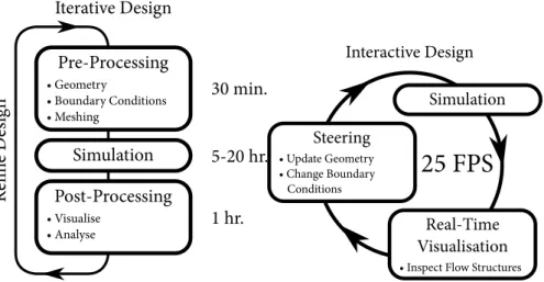
First and foremost, a real-time capability would give a completely new way to approach CFD problems. Nowadays a simulation with a typical CFD software is comprised of three key steps: (1) pre process-ing, (2) numerical simulation of the flow and (3) post-processing.

1. During the pre-processing step, the engineer defines the charac-teristic of the flow problem to be simulated by the solver in the next step. This is when the solution domain is defined, the phys-ical properties of the fluid are selected, the boundary conditions are specified and more importantly when the mesh required by the solver is generated. In itself, pre-processing can be a chal-lenging task, and a wrong choice of any of the aforementioned parameters might cause the solver to not properly converge. 2. The simulationis usually the longest step. The solver takes all

the parameters, boundary conditions and mesh from the pre-processor and simulate the flow using the selected equations and numerical method. It can range from a few minutes to sev-eral days for complex high resolution engineering applications. 3. Finally, the results of the solver are analysed during the

post-processing step. By its nature, CFD generates a large amount of data which requires specialised tool to dissect. A post-processor is basically a visualisation tool that can display informations in various forms such as vector, contour and surface plots but also compute additional flow informations that are not necessarily know to the solver such as vorticity, streamlines and streaklines. The post-processor generates images and animation and it is the role of the engineer to interpret the results of the simulation from them.

Each of these steps can easily take from a few minutes to a few hours depending on the application, but in a real-time context these steps need to happen several times per second. The geometry can be up-dated as the solver is running and the boundary conditions or even the fluid properties can be modified on the fly. A real-time visualisa-tion need to be connected to this process to inform the user on the changes that he is performing and allow him to inspect the resulting flow structures as they are being simulated. Typically, to avoid jit-tering and provide a smooth experience, a real-time fluid simulation need to be iterated at a minimum of25times per second, or frame per second (FPS) as for a film. Therefore, each simulation-step must take a maximum of 40 milliseconds to compute. The time constraints for real-time CFD are extremely tight. The Figure2 provides a

represen-tation of the design cycles using traditional CFD techniques against real-time CFD. It should be noted that the computing time figures are purely illustrative and would vary heavily depending on the applica-tion. • Geometry • Boundary Conditions • Meshing Simulation • Visualise • Analyse Post-Processing Pre-Processing 30 min. 5-20 hr. 1 hr. R e fi n e D esig n Iterative Design Simulation • Update Geometry • Change Boundary Conditions Steering

• Inspect Flow Structures Real-Time Visualisation

25 FPS

Figure2: Design cycles using traditional CFD versus real-time CFD.

The computational times provided are merely estimations for a simple indoor air flow simulation, and in practice they largely vary depending on the complexity of the simulation.

Real-time CFD and even “faster than real-time” CFD (the top

trian-computational time real-t ime c apab ility p h ysic al t im e slower than real-time faster than real-time Physical time of a problem versus the computational time required to solve it. gle on the figure in the margin) is necessary to inform early warning

systems. An example of such system, which is also amongst the only one to use predictive CFD, is weather forecasting. Weather forecast-ing relies on sensors for temperature, pressure and velocity spread across the surface of the country (but also in the air). These sensors are used to initialise the simulation, then the flow is solved on large clusters of computers, several times per day for both short-term and long-term forecasts. While the numerical methods used in weather forecasting vary depending on the country, in the UK the Met Office predictions come from aUnified Model which couples different simu-lations running on different grids at different resolutions (and

poten-tially with different numerical schemes). At its core, the solver uses a semi-implicit semi-lagrangian discretisation of the fully compressible Navier-Stokes equation on a rotating sphere, and meanwhile several additional processes operate to warm (or cool) and moisten (or dry) the atmosphere, to form clouds and precipitation.

Another area that has been hinted at and where real-time CFD would really help is in design optimisation. CFD is very often used by engineers in order to optimise one or several parameters of a model, from optimising the lift of an aerofoil to finding the optimal loca-tion for the ventilaloca-tion vents in a room. Optimisaloca-tion in CFD is very challenging because it requires to compute multiple simulations of the same problem, where the parameters to optimise are varied; and then, using clever techniques, guess the optimum based on interpo-lation of the limited set of simuinterpo-lations. There is an entire field of CFD devoted to that. Using real-time CFD, an engineer could vary the parameters to optimise by hand while monitoring the quantities of interest and quickly reach the optimal value for his problem. This process of modifying the simulation while it is running is known as computational steering.

Finally real-time CFD could bring a lot of benefits to teaching. Al-lowing the teacher to illustrate abstract concepts of fluid mechanics using real-time interactive simulations of real flows.

Maybe paradoxically, real-time simulation is easier to achieve for larger systems than for small ones. Indeed, while it is easy to solve planetary rotations due to gravity in real-time (one year to solve one rotation of the planet Earth!) it would be much harder (impossible) to solve microscopic particle collisions in real-time as they happen on very short time scales. The same is true with fluids, while it is possible (yet difficult) to simulate airflows around the globe in real-time, it would be harder to simulate a micro droplet impacting a surface in real-time. It is unlikely that real-time will ever be possible for such small time scales, and even if was it would not be very useful as the user would have to slow down the simulation to inspect the results. For such cases, it is more convenient to consider interactive CFDinstead which still yields many of the benefits detailed above. In1965, the

engineer Gordon Moore predicted that the doubling of component density on an integrated circuit (and thus the performance) every two years. Fifty years later, the law still holds, but its end might be near as components size approach that of the atom. Photo: Intel.

Nowadays, computers are very powerful machines and a single top-end desktop computer can easily achieve several teraFLOPS, that is several millions of millions of floating-point calculations per sec-ond. And yet, this is still insufficient to allow real-time simulation using traditional CFD methods (finite difference, volume, element), although it might become possible one day due to Moore’s law. In the meantime, it is necessary to come up with alternative methods, and maybe trade off some of the physical accuracy for higher compu-tational speed. The gaming industry and the computer graphics com-munity do not prioritise the physical accuracy, instead they use spe-cial numerical methods (usually wave-based or particle-based) that

looks convincing but do not resolve the Navier-Stokes equation. Al-though, in some cases, the semi-lagrangian scheme, which crudely approximate this equation, is used.

The most common way of faking a fluid in video games uses wave functions to apply oscillations on a surface, and create the illusion of a moving flow, but this hardly qualifies as a simulation. The second most commonly used technique for large water bodies solves for the shallow-water equation. When solely the surface of the water is of in-terest and the heights of the fluctuations are small compared the size of the water pool, the Navier-Stokes equation can be simplified by integrating along the depth. This technique allows to simulate con-vincingly waves propagating on the surface of the water and video games might use it to simulate waves on a pool around a character’s body, for instance. However, it is not amenable to indoor airflows.

Another way of approximating free-surface flows is using particles like in the smooth particle hydrodynamics (SPH) method. That tech-nique has gained popularity recently in video-games, despite its high computational cost, and NVIDIA, a large video-game company, re-cently developed a tool8

for real-time simulation using particles to represent both fluids, solids and soft bodies. The idea of SPH is to represent the fluid volume with particles that are advected using the simple Newton’s law and the particles are subjects to an interaction potential that tries to mimic surface tension. The technique is quite good at representing free surface flows like a dam breaking and its advantage is that it does not require a mesh (it is a meshless tech-nique) as the particles are allowed to move freely until they hit an obstacle. On the other hand, it does require a large number of parti-cles to accurately represent the flow and boundary conditions such as inlet/outlets are difficult to implement as particles have to enter/exit the flow domain. It is therefore not amenable to indoor airflows ei-ther.

Finally, thefast fluid method, also known assemi-lagrangian, is a grid-based method that relies on the Navier-Stokes equation where the advection term is approximated by guessing where the velocity of each cell is coming from, following the flow trajectory and using an interpolation scheme. The method is very interesting due to its good computational efficiency and unconditional stability, as showcased by its successful use in weather forecasting. However, it is relatively inaccurate in its standard form but there are several possible modifi-cations that aims at improving its accuracy (although they require to loose some of its simplicity, efficiency and stability). More details on the method will be given in AppendixC.

Another contender for real-time CFD, although it is very rarely used in computer graphics, is the lattice Boltzmann method(LBM). As a numerical method, the LBM can be regarded as an explicit scheme

second order in space and first order in time. Its explicit nature makes the method very computationally efficient, but its real particularity is that it does not solve directly for the Navier-Stokes equation or for an approximated version of it. Instead, the LBM solves for a discrete ver-sion of the Boltzmann equation, an equation coming from the kinetic theory of gases. The LBM shows several advantages : it is simple, fast (especially on parallel processors, see chapter4), stable and it can

ac-curately solve for thermal and turbulent air-flows making it an ideal candidate as the preferred numerical scheme in the real-time simula-tion of indoor air-flow for this Ph.D. As a result, after introducing the method in the next section, chapter 2 will give a detailed review of

the method, including some of its many variants, chapter3identifies

various boundary conditions and chapter4will discuss its optimised

implementation on a Graphics Processing Unit. 1.4 l at t i c e b o lt z m a n n m e t h o d (l b m) microscopic scale mesoscopic scale LBM Navier-Stokes Particle Methods velocity, pressure distribution functions particles position and momentum

Figure3: A fluid flow can be studied from various scales.

Three length scales (or time scales) can be defined for a fluid flow : the microscopic scale, the macroscopic scale and between the two an intermediary scale named : mesoscopic scale. These scales are repre-sented in figure3.

m i c r o s c o p i c s c a l e This is the scale of the molecules of fluid. At this scale, particles have ballistic trajectories (Brownian motion) with an average microscopic speed given by the temperature. This is the scale that molecular dynamics and smooth particle hydrodynamics try to replicate to some extent.

m e s o s c o p i c s c a l e When the number of particles becomes large, it becomes more convenient to average the particles over a vol-ume. The kinetic theory studies the evolution of particle’s distri-bution function. Distridistri-bution functions exist in phase space, for instance f(~x,~u,t) represents the number of particles per unit volume having the velocity ~u within the volume surrounding

the location~xand at timet. It is this mesoscopic viewpoint that is taken by the LBM.

m a c r o s c o p i c s c a l e This is the scale of the variations of vectors fields (like the fluid speed~u) and scalar fields (like the pressure

p or the temperature T). This scale is large enough compared to the microscopic and the mesoscopic scale that the fluid can be considered as a continuum substance, so that macroscopic quantities are defined on every point~x and every time t. For instance, the speed can be written as~u(~x,t)and the pressure as

p(~x,t). The behaviour of these macroscopic fields is described accurately by the Navier-Stokes equation.

While it might seem strange that the LBM, focused on particle’s dis-tribution function, can be used to simulate macroscopic flows, such as indoor airflows, that are normally described by the Navier-Stokes equation, the two methods do in fact produce the same results, and with a similar accuracy, see chapters 6 and 7. Actually, it has been

shown that the Navier-Stokes equation can be derived from the lattice Boltzmann equation through a low Mach number expansion known as the Chapman–Enskog procedure[3].

It is important to note that the LBM is not a single method but rather a category or group of methods that can be used to solve di-verse partial differential equations (not just the incompressible Navier-Stokes). This can make LBM confusing to the beginner, as it can be difficult to choose which variant of the method to use for which problem. On the other hand, it is this flexibility that make the LBM so powerful allowing to simulate the incompressible Navier-Stokes equation for isothermal single phase flow but also other problems like multiphase flows using an interaction potential or completely different problems such as solving the light transport equation[4, 5]

or the Schrödinger equation for quantum dynamics[6].

One of the strong point of LBM compared to traditional CFD (based on Navier-Stokes) is that it does not require to solve a Poisson equa-tion for the pressure. This allows the LBM to be intrinsically local, i.e., each node can be computed independently from its neighbours, which in turn results in very high performance when implemented on a massively parallel processor like a GPU (see next section). A down-side though, is that it comes at the price of a generally less accurate pressure field and small variations in density that can cause pressure waves. In this regard, the LBM is an artificially compressible scheme to solve the incompressible Navier-Stokes equation, rather like the artificial compressibility method(ACM)[7].

On the other hand, one of the downsides of LBM is itsyouth com-pared to most other numerical methods in CFD. A direct consequence of that is that the LBM still requires some development work (for in-stance in the modelling of the turbulence) as well as a serious work ofclassificationandstandardisation. Notably on the implementation of

the boundary conditions or on the process of unit conversion which is too often overlooked (that is the process of transforming the macro-scopic variables defining a problem into an initial state and boundary conditions for the distribution functions used in the simulation).

The LBM is a very active field of research, and as such, there are two yearly international conferences dedicated to it, hosted by differ-ent universities each year. The Discrete Simulation in Fluid Dynam-ics9

(DSFD), which is more focused on the theoretical development of the method. And the International Conference for Mesoscopic Methods in Engineering and Science10

(ICMMES) which features rel-atively more engineering-focused applications. In the United King-dom, the UK Consortium on Mesoscale Engineering Science11

(UK-COMES) aims to bring together the expertise from multiple univer-sities in the UK and to maintain DL_MESO12

, a simulation package based on LBM (free for academics).

Commercial LBM software

Due to its originality and youth, the LBM is not yet very popular amongst CFD engineers, as a result there are only a few commercial CFD software based on LBM.

u lt r a f l u i d x 13 : developed by the German company FluiDyna GmbH which also develops an SPH software, a finite volume software and a library for GPU acceleration of OpenFOAM. The company is investing in GPU computing and all its software feature GPU acceleration, allowing large performance increase. The ultraFluidX software is mostly dedicated to the simulation of airflows around moving vehicles, it features turbulence mod-elling, a mesh refinement technique and it allows for in-situ visualisation.

p o w e r f l o w 14: developed by the American company Exa Corpora-tion and also focuses on the simulaCorpora-tion of airflows around vehi-cles. The company product line include a tool to study the noise created by the interaction of the air and the moving vehicle and a tool for thermal management as well as several dedicated soft-ware for pre or post processing.

x f l o w 15: developed by the Spanish company Next Limit S.L which also develops fluid simulation software for the graphics

indus-9 http://www.dsfd2015.ed.ac.uk/home 10 https://www.icmmes.org 11 http://www.ukcomes.org/ 12 http://www.stfc.ac.uk/SCD/support/40694.aspx 13 http://www.fluidyna.com/content/ultrafluidx 14 https://www.exa.com/powerflow.html 15 http://xflowcfd.com/

try and a physically based image renderer for architecture ap-plications. The solver is based on the factorised central moment LBM and features an LES turbulence model (with special wall modelling). It allows moving boundaries with adaptive wake refinement and can simulate multiple fluid physics such as com-pressibility, thermal fluctuations, turbulence, multiphase flows, etc...

pa l a b o s 16 : Palabos is an open-source solver developed by the a commercial company FlowKit Ltd. from Switzerland. It has a reasonably large community from academia with an active forum17

and a wiki18

full of useful information for beginners looking to get started with LBM. The source code is written in the C++ programming language and relies heavily on tem-plates for compile time optimisation. It features a large variety of models such as multi-phase/free-surface flow, thermal flow, fluid-particle interaction and immersed moving object. It uses a multi-block technique for mesh refinement and can scale well with the number of cores, however it does not feature GPU ac-celeration.

Due to the simplicity of its algorithm LBM also spawned a large amount of open-source implementations, usually developed by a sin-gle person and thus not very well maintained and limited in reach. Nonetheless, the Sailfish19

project is particularly interesting as it uses Python (a scripting language) to maintain the ease of use and gener-ates an compilable code (C or CUDA) to achieve high performances, and it works on GPU. A similar approach was used for the develop-ment of the simulation code for this Ph.D.

1.5 g r a p h i c s p r o c e s s i n g u n i t (g p u) The GTX Titan X from NVIDIA. With6teraFLOPS of compute power, it is amongst the fastest computer chip to date. Photo: NVIDIA. A graphics card, also known as graphics processing unit, or GPU for

short, is a recent type of processor that focuses on parallel computing. Traditionally, this type of computing device was found in video game consoles and in gaming PC to accelerate the graphics computations. Their functioning is significantly different to that of a central pro-cessing unit (CPU) which handles of all of a computer’s processes. While the CPU has to handle a large variety of tasks in a iterative way, the GPU operations are more specialised and done in parallel so that every pixels of the display is computed at the same time, for instance. Over the last fifteen years, the architecture of the GPU has evolved independently from that of the CPU and they are nowadays

16 http://www.palabos.org/ 17 http://www.palabos.org/forum/ 18 http://wiki.palabos.org/

much more powerful than their CPU counterpart. Both in term of raw compute power, as they pack a massive amount of cores (a few thousands versus a dozen for a CPU), but also in term of memory bandwidth, that is the speed at which data can be accessed, using their own dedicated memory. They can come in multiple forms or shape, size, performance and price, but overall they are more inter-esting than CPUs in term of performance per watt (power usage) and performance per price.

On the other hand, a program needs to be written carefully in a special programming language in order to run efficiently on a GPU, it is not possible to just run a program compiled for a CPU. Even so, the LBM can be implemented very efficiently on the GPU (as de-scribed in chapter4), achieving a performance of more than a billion

cell updates per second for a 3D problem, opening the door to the simulation of complex indoor airflows in real-time.

1.6 o b j e c t i v e s o f t h e t h e s i s

This thesis is in line with two research themes from two different insti-tutes at the University of Leeds. Namely the Institute of Thermoflu-ids in the school of Mechanical Engineering looking at the thermal management of data centres and the Institute for Public Health and Environmental Engineering with an interest on the control and the optimisation of hospital ventilation.

The goal of this project is to develop a real-time capability for the simulation of thermal and turbulent indoor air flows, running on a single (high-end) desktop computer.

To this purpose, the lattice Boltzmann method is used as the main numerical method for the solver, as it is more efficient than methods that discretise the Navier-Stokes equation, while being as accurate.

Moreover the solver is implemented and optimised on a GPU, al-lowing a computational speed increase of about two orders of magni-tude compare the same implementation on the CPU.

The software needs to be able to handle the complex geometries of indoor environment as well as being able to accurately model the thermal and turbulent fluid behaviours while maintaining the real-time capability. In addition, it needs to provide a facility for an easy definition of the fluid flow problem with its geometry and appropri-ate boundary conditions together with an in-situ visualisation tool to allow for the real-time study of the flow as it is simulated and to allow for computational steering from user inputs.

The finished software could have multiple applications in engineer-ing but two applications are of particular interest. (1) The prediction and control of thermal loads indata centres(see section7.3) as well as

the optimisation of the ventilation system design in order to reduce the cost of the cooling. The tool could be combined one day with

sen-sors and actuators located inside a data centre to allow for dynamic adaptive cooling based on the servers load and the temperature pro-file across the room. (2) The simulation of the ventilation in hospital wards (see section7.4) in order to improve the thermal comfort of the

patients and predicting the transport of pollutants (such as dust, bac-teria and viruses) in the hope of creating one day smart hospitals that would be able to respond quickly to the spread of a contamination. 1.7 t h e s i s o u t l i n e

Chapter2 of the thesis provides an extensive description of the field

of LBM in its current state, with details on multi-physics modelling (multi-phase or thermal coupling), on improved collision operators for increased stability, on turbulence modelling and on techniques to approach non-uniform grids.

Chapter 3 then extend the description with an important

discus-sion on the issues of initial and boundary conditions that any LBM implementation must deal with.

Chapter4introduces the graphics processing unit and the concepts

of parallel programming. It describes the implementation of each LBM model on the GPU and their optimisation in order to achieve the highest computational throughput. This implementation is then tested in chapter5for its performances and chapter6for its accuracy

against various benchmark problems.

Chapter 7 applies the described software and algorithms to the

simulation of indoor airflows by looking at a benchmark room for the ventilation and at a the modelling of a small data centre.

Finally, chapter 8 showcases how the program has the potential

to be applied to a wider range of applications and presents some results on multiphase flows, on fluid-structure interactions and on the parameter search for enhancing the stability in some moment-based models.

2

2.1 i n t r o d u c t i o n

This chapter delves into the lattice Boltzmann method (LBM), its ori-gins as a cellular automaton, its foundations in kinetic theory, and the general framework of the method; more details on the algorithm and boundary conditions will be given in the next chapter. The current chapter is an attempt at a comprehensive classification of the large variety of models developed over the years for multi-physics appli-cations. It includes a presentation of the alternative collision opera-tors designed to improve the stability and accuracy over the standard LBM, as well as a discussion on some of the techniques for turbulence modelling and mesh refinement, both important topics for indoor air flows modelling.

2.1.1 Historical background

The Boltzmann equation (see details in section 2.1.3) describes gas

behaviour through the statistical distribution of fluid particles. In 1973, Hardy, Pomeau, anddePazzis[8] had the idea to render both

velocities and locations of the particles discrete by using a cellular

au-tomaton, known nowadays as the lattice gas automaton. Later, in1986, _{A cellular} automaton, like the popularConway’s Game of Life[9], consist of a regular grid of cells, each which a finite number ofstates. Complex behaviours can emerge from the simple updating rules.

Frisch, Hasslacher and Pomeau[10] provided the first lattice gas

automaton that was able to recover the Navier-Stokes equation. They showed that when the collision rules conserve mass and momentum, and if the underlying lattice has a sufficient symmetry (at least hexag-onal in two dimensions) then the lattice gas automaton can lead to the Navier-Stokes equation in the macroscopic limit [11].

In order to fix the issue of the high statistical noise with the lat-tice Boltzmann automaton (i.e. one of its main drawbacks), a new model was first introduced by McNamaraand Zanettiin1988[12]:

the Lattice Boltzmann Equation. The basic idea is simple: replace the Boolean variables (corresponding to a single Boolean molecule) of the cellular automaton by floating point variables (corresponding to the distribution function of molecules). Then in1989, Higueraet al. [13,14] showed that using a linearised form of the collision

opera-tor increases significantly the accessible Reynolds numbers.

While by then, the core of what would become the lattice Boltz-mann method(LBM) was founded, a very significant progress has been made over the last 25 years, both in term of the theory, applications and performances. While the lattice gas automaton started as an

em-pirical model to replicate fluid flow behaviour, the theoretical foun-dations of the LBM are now sound : it is now clear in which limits the Navier-Stokes equations are recovered [15,16,17] and the role of

the artificial compressibility is better understood [7]. Many models

have been proposed [18, 19, 20, 21] to increase the accuracy and

nu-merical stability of the LBM over the original implementation. This has somehow fragmented the LBM into many different models, as section2.4tries to convey, so much that it seems necessary to address

the LBM as the lattice Boltzmann methods (with a plural). These LBM(s) have been employed in many areas with success, such as flows in porous media [22,23], turbulent flows [24,25,26,27,28],

mul-tiphase flows [29], thermally driven flows [30, 31, 32, 33],

compress-ible flows [34], electronic kinetic flows [35,36],

magnetohydrodynam-ics [37], non-Newtonian flows [38], soft matter systems [39], shallow

water flows [40], reaction and combustion [41], radiation heat

trans-fer [42], relativistic hydrodynamics [43], quantum mechanics [6] and

so on.

The last twenty years have seen a massive improvements on the at-tainable computational throughput as the machines, algorithms, and implementations have evolved [44,21,45]. In the recent years, the rise

of the graphics processing unit as a general purpose computing plat-form has opened the road to accurate fluid simulation in real-time and in an interactive way [46].

Despite the scepticism at its beginnings (and some that still per-sists today), the LBM is now accepted by the scientific community as a viable way to simulate fluid flows, although its adoption by the engineering community is rather limited, mostly due to the lack of established commercial software. Its numerical stability, physical ac-curacy, adaptivity to multiple problems and its numerical efficiency on multi-core architecture makes it the ideal candidate for the future generation of fluid flow solvers [47].

2.1.2 Kinetic Theory

Kinetic theory is the branch of statistical mechanics dealing with the dynamics of non-equilibrium processes and their relaxation to ther-modynamic equilibrium. At its foundation, the theory is based on themolecular hypothesisof matter, which postulates that matter is not continuous but is composed of a large (but finite) number of small bodies, called molecules. The theory explains macroscopic properties of gases, such as pressure, temperature, viscosity, thermal conduc-tivity, etc., by considering the microscopic motion of the constituent molecules.

In ordinary mechanics, the aim is usually to determine the events that follow from prescribed initial conditions. This approach is not viable for the kinetic theory of gas because (i) the detailed state of

mo-tion of every molecules at an initial instant is unknown and (ii) the

sheer number of molecules is too large (in the order of the Avogadro _TheAvogrado

constant, that is the number of molecules in one mole, is of the order of1023which largely exceeds the capacity of even the largest super-computers in the world (around1016 flops).

constant) to allow to follow the subsequent motion of all the many molecules that compose a gas. Hence kinetic theory does not even at-tempt to consider the fate of individual molecules, but instead is only interested in their statistical properties, such as the mean number, momentum or energy of the molecules within an element of volume, averaged over a short time interval. This point of view is necessary because of the computational limitations but it is also physically ade-quate, as experiments only measure such averaged properties.

Hence, in statistical mechanics a gas is described by the distribution function of its moleculesf(~x,~u,t)which represents the probability of finding a molecule at the position~x, with the velocity ~u, at the time

t. Macroscopic laws of the evolution of gases can be predicted by the molecular description of kinetic theory and one its main success was to predict the second law of thermodynamics, one of the most fundamental laws of nature which states that the entropy of a closed system is always increasing.

2.1.3 The Boltzmann Equation

The Boltzmann Equation is the cornerstone of kinetic theory, it

de-Ludwig Eduard Boltzmann (1844–1906) was an Austrian physicist whose greatest achievement was in the development of statistical mechanics, which explains and predicts how the properties of atoms determine the visible properties of matter. Image source: The Dibner Library Portrait Collection -Smithsonian Institution Libraries. scribes the evolution of the distribution function f(~x,~u,t) in terms of

micro-dynamic interactions. This equation was derived in1872by the Austrian scientist Ludwig Boltzmann. And although this equation was established more than a century ago, the formal mathematical proof of global existence and rapid decay to equilibrium of classical solutions was only achieved recently, in2011[48].

The Boltzmann Equation for the one-body distribution function

f(~x,~u,t)can be written as:

∂t+~u.∇~x+~F.∇~p

f(~x,~u,t) =C12 (6) where the left-hand side represents the streaming motion of the molecules along the trajectories associated with the force field ~F (a straight line if ~F = ~0) and C₁₂ represents the effect of (two-body) intermolecular collisions taking molecules in and out of the streaming trajectory. It is assumed that encounters with other molecules occupy a small part of the lifetime of a molecule, this implies that only binary encounters are important.

The termC₁₂represents the collision integral of two particles, hence the name collision operator; it acts only on the velocity ~uand is local in the position~xand timet. While the Boltzmann collision operator can take various forms, as the Boltzmann Equation is applicable to a large variety of systems, for a dilute gas of point-like and