Phase-retrieval algorithm for the characterization of broadband single attosecond pulses
Xi Zhao,1,2Hui Wei,1Yan Wu,1,3and C. D. Lin1,*1Department of Physics, Kansas State University, Manhattan, Kansas 66506, USA
2Laser Fusion Research Center, China Academy of Engineering Physics, Mianyang, Sichuan 621900, People’s Republic of China 3School of Science, Zhejiang Sci-Tech University, Hangzhou 310018, People’s Republic of China
(Received 17 February 2017; published 10 April 2017)
Recent progress in high-order harmonic generation with few-cycle mid-infrared wavelength lasers has pushed light pulses into the water-window region and beyond. These pulses have the bandwidth to support single attosecond pulses down to a few tens of attoseconds. However, the present available techniques for attosecond pulse measurement are not applicable to such pulses. Here we report a phase-retrieval method using the standard photoelectron streaking technique where an attosecond pulse is converted into its electron replica through photoionization of atoms in the presence of a time-delayed infrared laser. The iterative algorithm allows accurate reconstruction of the spectral phase of light pulses, from the extreme-ultraviolet (XUV) to soft x-rays, with pulse durations from hundreds down to a few tens of attoseconds. At the same time, the streaking laser fields, including short pulses that span a few octaves, can also be accurately retrieved. Such well-characterized single attosecond pulses in the XUV to the soft-x-ray region are required for time-resolved probing of inner-shell electronic dynamics of matter at their own timescale of a few tens of attoseconds.
DOI:10.1103/PhysRevA.95.043407
I. INTRODUCTION
In the last decade and half, significant attention has been devoted to the development of attosecond science and technol-ogy, in particular, the generation of attosecond pulses and how they can be used to probe dynamics of electrons at the ever-shorter timescale, for atoms, molecules, and nanostructure ma-terials [1]. Various techniques have been developed to generate broadband extreme ultraviolet (XUV) light that has available continuum bandwidth capable of supporting pulse durations of a few tens to hundreds of attoseconds, such as amplitude gating [2], ionization gating [3], polarization gating [4], double optical gating [5], and the wavefront rotation method [6]. Similarly, by using few-cycle phase-stabilized mid-infrared wavelength lasers, ultrabroadband supercontinuum harmonics up to the water-window and beyond have been reported [7–15]. If these pulses are transform limited, the resulting durations of the attosecond pulses are expected to range from 30 attoseconds down to even a few attoseconds. However, it is well known that high-order harmonics generated in a gas medium exhibit attochirps [16]. Over the broadband, the chirp can be quite significant if the phase has not been compensated [17]. Clearly, full temporal characterization of these pulses is needed. Unfortunately, it cannot be carried out with the current pulse measurement techniques.
Attosecond pulses with durations of 67 as [18] or 80 as [2] have been reported by using typical 800 nm driving lasers. These pulses are characterized based on the principle of attosecond streaking where the XUV electric field is converted to an electron spectrum, or spectrogram, through photoelectron emission in atoms, in the presence of a moderately intense IR laser field. In the streaking spectrogram, the momentum of the electron is shifted by an amount depending on the relative time delay between the XUV and the IR pulses. Thus time information of the attosecond pulse is encoded in the amount
of momentum shift in the streaked spectrogram. A standard technique known as frequency-resolved optical gating for complete reconstruction of attosecond bursts (FROG-CRAB) [19–21] has been used to retrieve the attosecond pulse, which stems from the FROG method for the characterization of femtosecond infrared laser pulses. The retrieval is based on an iterative process by matching the measured photoelectron spectrogram to a FROG-CRAB trace from an unknown XUV pulse and an unknown IR field.
FROG-CRAB employs a number of approximations. The most damaging one is the so-called “central momentum approximation,” which limits its applicability only to narrow-bandwidth pulses, i.e., the approximation is reasonable only when the bandwidth of the attosecond pulse is much smaller than the central energy of the photoelectron. This approxi-mation is required to be able to adopt the existing inversion algorithm used in FROG, which was widely used for femtosec-ond laser pulse characterization. The failure of FROG-CRAB for retrieving broadband attosecond pulses is well known. An earlier phase retrieval by omega oscillation filtering (PROOF) method was proposed for such pulses [22]. However, the method relies on a relatively long and weak streaking IR pulse, and that the dipole moment within the bandwidth is assumed to be constant. These approximations, as addressed by Weiet al.[23], are not consistent with broadband pulses that span many tens to hundreds of electron volts. Very recently, it has come to our attention that a method called “Volkoff transform” generalized projections algorithm (VTGPA) has been proposed to retrieve broadband XUV attosecond pulses in the IR streaking field [24], but the VTGPA has not been extensively tested yet and has not been applied to soft-x-ray attosecond pulses or to mid-infrared streaking lasers.
In this article, we report an iterative retrieval algorithm that does not employ the central momentum approximation. An iterative procedure is still employed but, for efficient convergence, efforts were made to reduce the number of unknown parameters in the guessed electric fields of the XUV and the IR. We take advantage of pulse parameters
that can be measured from other experiments; for example, the spectral amplitude of the XUV pulse which in general can be obtained from photoionization measurement by the XUV alone. The IR phase and/or amplitude can be assumed to be known or unknown depending on the nature of the measurement. We choose to expand the unknown amplitude and/or phase of the XUV and the IR fields in terms of the so-calledB-spline basis functions [25]. Such expansions are commonly used in representing a smooth function with a minimum number of unknowns. We call our method phase retrieval of broadband pulses (PROBP), since the method can not only retrieve broadband single attosecond pulses in the XUV or soft x-rays, but also retrieve wide-band infrared streaking fields spanning over a few octaves that are used to generate supercontinuum harmonics [26–28]. In Sec. II we briefly introduce the PROBP method, including the strong-field approximation (SFA) on which this method is based, and the way to construct unknown functions by using theB-spline basis. In Sec.IIIwe simulate the photoelectron spectrograms in various experimental conditions, and then test the accuracy of the PROBP method in retrieving the single attosecond pulse as well as the streaking IR field. Finally we summarize this article in Sec.IV. Atomic units are used unless noted otherwise.
II. PRINCIPLE OF PHASE RETRIEVAL OF BROADBAND PULSES A. Strong-field approximation
Both the FROG-CRAB, VTGPA, and PROBP methods assume that the measured photoelectron spectrogram can be modeled by the SFA [19,20]:
S(p,τ)= ∞ −∞ EXU V(t−τ)d[p+A(t)] ×e−i(p,t)ei(p 2 2+IP)tdt 2 , (1)
where EXU V(t) is the XUV or the soft-x-ray field to be characterized. For simplicity we use XUV to include soft x-rays, and IR to include mid-IR in the following unless otherwise specified. τ is the time delay between XUV and IR,d(p) is the transition dipole between the initial bound state and final continuum state of the atom. The vector potential of the IR isA(t)= −−∞t EI R(t)dtand the phase function (p,t) reads (p,t)= ∞ t pA(t)+A 2(t) 2 dt. (2)
The polarization directions of the XUV, the IR and the direction of the photoelectrons are all taken along the zaxis. In the FROG-CRAB method, a central-momentum approximation was imposed on Eqs. (1) and (2), where(p,t) is replaced by (p0,t), andp0is the central momentum of the photoelectrons. In PROBP (and in VTGPA) no such approximation is imposed. In our method, the XUV pulse in the energy domain is expressed as
EXU V()=U()e−iφXU V(). (3)
A single color, multicycle IR field in the time domain is expressed as
EI R(t)=f(t) cos [ωLt+ϕI R(t)], (4) while a broadband IR pulse consisting of multiple colors is better represented in the frequency domain
EI R(ω)=A(ω)e−iφI R(ω). (5)
In this work, we assume that the amplitude and phase of the transition dipole d(p) is known. In our simulations Ne is chosen as the target, modeled by a single-electron model potential [29]. Therefore, the transition dipole d(p) can be calculated accurately. We always use IR peak intensity at 1013 W/cm2 and XUV at 1012 W/cm2. The actual intensity of the latter is not important since the XUV enters Eq. (1) linearly. We also assume that the spectral amplitude of the XUV, i.e.,U(), is known since it can be extracted from XUV photoionization experiments without the IR.
B. Expanding unknown functions by usingBspline In the simulations, the “experimental” spectrogram is obtained with known input XUV and IR fields. Our goal is to retrieve the phase of the XUV, i.e., φXU V(), as well as the IR field as if they were unknown. The IR field can be retrieved either in the time domain with unknown functionsf(t) and ϕI R(t), or in the frequency domain with unknown functions A(ω) and φI R(ω). Therefore, there are three unknown functions in total. Each unknown function is expanded in terms ofB-spline basis functions.
In general, a smooth functionf(x) can be expanded as
f(x)= n
i=1
giBik(x), (6)
wheregi are expansion coefficients, andiis the index of the B-spline function. The kth ordersB-spline functions Bik(x) are defined through
Bi1(x)= 1, xi xxi+1 0, otherwise, (7) Bik(x)= x−xi xi+k−1−xi Bik−1(x)+ xi+k−x xi+k−xi+1 Bik+−11(x). (8)
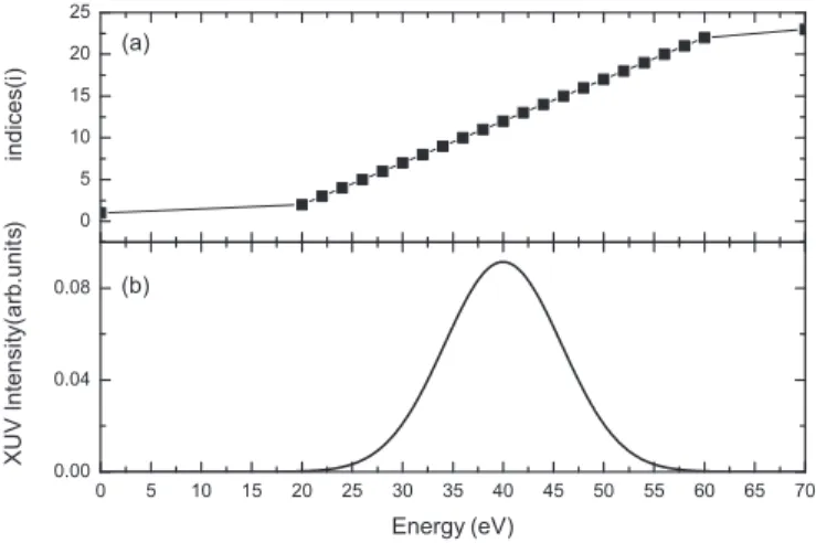
Here {xi} are the knot points. If there are n B-spline basis functions of the order k, the total number of knot points is n+k. The B-spline function is a powerful tool for fitting a smooth function [25], and it has been widely used in computational physics. Figure1shows an example where the input smooth function is accurately reconstructed by seven B-spline basis functions by optimizing the knot points and the expansion coefficients. The red solid line is the function to be fit while the black dash line corresponds to the reconstructed function. The typicalB-spline basis functions are also shown in the graph.
In our situation, we define the guessedB-spline expansion coefficients for the three unknown functions as{ai},{bi}, and
{ci}, respectively. From these coefficients the guessed XUV and IR fields can be constructed, and then for each discrete set of points{Ek,τl}the corresponding spectrogram is obtained by using Eq. (1). Typically we chose 100 to 500 points in time
FIG. 1. Illustration of expanding a smooth function in terms ofB-spline basis functions. The input function (red solid line) is compared with the reconstructed one (black dashed line). Seven B-spline functions with the order of five are used in the reconstruction. delay and 100 points in energy. The error function is defined as
E[ai,bi,ci]= k,l
[S0(Ek,τl)−S1(Ek,τl)]2, (9) whereS0andS1are the input and reconstructed spectrograms, respectively. We use the genetic algorithm (GA) to find the optimal parameters {ai,bi,ci} that would minimize Eq. (9). The GA runs a large number of generations (typically 50 000 to 100 000 generations) until convergence is achieved. The optimal parameters{ai,bi,ci}are then used to reconstruct the XUV and IR pulses.
The convergence of the retrieval algorithm depends on how we choose the numbernand the orderkof theB-spline basis and how we place the knot points {xi} for each unknown function. If we know the spectral amplitude of the XUV pulse; for example, see Fig.2(b), then in order to retrieve the spectral phase of the XUV, more knot points can be placed within the
FIG. 2. The scheme that shows how we optimize the distribution of the knot points (a) for XUV phase based on the spectral amplitude of the (b) XUV pulse.
spectral range of the XUV and less outside, as illustrated by Fig. 2(a). Since the spectral amplitude and phase of the IR are not known, the knot points are distributed more evenly for both functions.
Because there are three unknown functions constructed by three sets ofB-spline functions, each with its own parameters nandk, the optimization is carried out as follows: First, we search the bestn1andk1by fixing a given collection ofn2,k2, n3,k3. We scan all possiblen1andk1in the GA and calculate the error after a few generations, for example, 100 generations. The combinationn1andk1which leads to the smallest error is documented. Next, we perform the same procedure to find the bestn2,k2by fixingn1,k1,n3,k3, in whichn1,k1have been optimized in the first step already. Third, we find the bestn3and k3by using then1,k1,n2,k2obtained from the previous steps. The whole process can be repeated for several times. Once we find the best ni andki, (i=1,2,3), the GA converges very fast and the optimization is very efficient. In our simulations, it only takes about 30 minutes to get converged results. Below we illustrate various results from our simulations.
III. SIMULATIONS AND RESULTS A. Equivalence of PROBP and FROG-CRAB for
narrow-bandwidth attosecond pulses
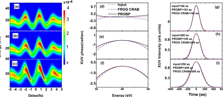
In the first simulation, we consider three XUV pulses, each with central photon energy of 40 eV and spectral width of 11 eV. The spectral width is always referred to the full width at half maximum (FWHM). The IR pulse has a central wavelength of 800 nm and a duration of 4.4 fs. In this example the spectrogram is calculated by solving the time-dependent Schrödinger equation (TDSE) instead of using Eq. (1). This allows us to test how SFA affects the accuracy of the retrieval of the XUV phase. The three XUV pulses differ only by their spectral phases. The first one is transform limited, with a duration of 160 as. The second and third are chirped with durations of 200 and 250 as, respectively. Figure3documents the results of the simulation. Along the left column, the spectrograms are shown. The differences among them are quite discernible. By using the FROG-CRAB and PROBP methods the XUV phase for each pulse is retrieved (the amplitude is set to be the input one), as shown in the middle column. Clearly the phases are accurately retrieved except near the wings where the spectral amplitude is already small. Nevertheless it does show that PROBP is closer to the input phase. From the known spectral amplitude and retrieved phase, the temporal intensity of each XUV pulse is obtained; see the right column. They all agree very well with the input pulses. This example shows that Eq. (1), even though it is an approximate theory, can still be used to retrieve the XUV pulses.
B. Broadband XUV pulses where FROG-CRAB fails For a transform-limited attosecond pulse with duration of one atomic unit, i.e., 24 as, the bandwidth is 75 eV. In this example, we consider a chirped XUV pulse with a duration of 52 as, a central photon energy of 80 eV, and a bandwidth of 90 eV. The input XUV phase is shown as the red dash line in Fig. 4(a). The SFA, Eq. (1), was used to simulate the spectrogram with the IR given in Sec. III A. By using
FIG. 3. Characterization of three XUV pulses centered at 40 eV with a bandwidth of 11 eV. The FWHM durations of these pulses are 160, 200, and 250 as, respectively. Panels (a)–(c) show the input spectrograms simulated by TDSE, with the three XUV pulses. Panels (d)–(f) show the spectral phases of the three XUV pulses. Panels (g)–(i) show the XUV intensity profiles in the time domain. The red dash lines are the input data, the black solid lines are retrieved from the PROBP method, while the blue dash-dot lines are retrieved from FROG-CRAB.
FROG-CRAB, the retrieved XUV spectral phase, displayed as the blue dash-dot line in Fig.4(a), shows significant deviation from the input phase, while the present PROBP (see black solid line) is capable of retrieving the highly modulated spectral phase. The reconstructed temporal profiles, as shown in Fig. 4(b), reveal that the FROG-CRAB method fails to reproduce the chirp of the input pulse. It predicts a pulse duration of 25 as, while the PROBP method recovers a pulse duration of 51 as, as compared to the input value of 52 as,
FIG. 4. Comparison between FROG-CRAB and PROBP for characterizing an XUV pulse centered at 80 eV with a broad bandwidth of 90 eV. Panel (a) shows the XUV spectral phase. Panel (b) shows the XUV intensity profile. The red dash lines are the input data, the black solid lines are retrieved from the PROBP method, while the blue dash-dot lines are retrieved from the FROG-CRAB.
as well as a good agreement of spectral phase over the whole bandwidth. This example testifies to the severe failure of the central-momentum approximation used in the FROG-CRAB method, and the success of the PROBP method for a broadband XUV pulse.
C. Phase retrieval of attosecond pulses in water-window region High-order harmonics in the “water window” with photon energy ranging from 280 to 530 eV have been reported in a number of laboratories in recent years [7–15]. Such soft-x-ray harmonics are needed to excite core-level transitions in materials. They are generated by long-wavelength mid-infrared lasers using an optical parametric amplification (OPA) or optical parametric chirped-pulse amplification (OPCPA), pumped by a Ti-sapphire laser. When generated with few-cycle mid-infrared lasers it has been found that the generated harmonics exhibit a supercontinuum spectrum, with the possibility of supporting single attosecond pulses of durations of less than thirty down to a few attoseconds. However, due to the atto-chirp of the generated harmonics, without post-phase compensation, it is fortuitous to claim single attosecond pulses with such short durations. Unfortunately, since the prevalent FROG-CRAB method is not expected to be valid for retrieving broadband attosecond pulses, pulse duration of attosecond pulses in the water-window region has not been retrieved so far. In this example, we choose three input attosecond pulses with central energy of 300 eV and bandwidth of 46 eV. In the transform-limited case this spectrum will support a pulse duration of 46 as. The three input XUV pulses differ by their spectral phases; see Figs.5(a),5(c), and5(e). We assume that the soft-x-ray harmonics are generated by a four-cycle 2000 nm mid-infrared laser which is also used as the streaking field. In this example, we have not been able to obtain converged results for the spectral phase by using FROG-CRAB. On the
FIG. 5. Phase retrieval of soft-x-ray pulses centered at 300 eV with a bandwidth of 46 eV using PROBP. Left column shows spectral phases of three different soft-x-ray attosecond pulses. The spectral amplitudes for the three pulses are identical. Right column shows the temporal intensity of the three pulses. The red solid lines are the input data and the black dash lines are retrieved from the PROBP method. The XUV pulses are centered at 300 eV with a bandwidth of 46 eV. The wavelength of the dressing mid-IR field is 2000 nm, and the duration is four cycles.
other hand, with the PROBP method, we have successfully retrieved the spectral phases for all the three cases. The resulting temporal intensity for each pulse has also been successfully retrieved; see Figs.5(b),5(d), and5(f). The input pulse durations of the three examples are 436, 147, and 46 as, to be compared to the durations retrieved from the PROBP of 419, 156, and 50 as, respectively.
Besides the central-momentum approximation, the FROG-CRAB algorithm we used [20] relies on the discretization of the time axis. Using mid-infrared lasers as the streaking field,
the phase (p,t) in Eq. (2) grows like λ2, thus the factor e−i(p,t)in Eq. (1) oscillates very rapidly, and it would require a very small time stepdt in the integration to less than 1 as. In the FROG-CRAB algorithm, the time domain and energy domain are related by the fast Fourier transform (FFT), which imposes a sampling condition dt dE=2π/N. Here dE is the energy step and N is the number of data points in both time and energy domains. If we also limit the energy stepdE to less than 0.1 eV, then N should be greater than 40 000. For such a large data set, it will take an unaffordable time for FROG-CRAB to get a converged result. This makes the current FROG-CRAB retrieval method not applicable for mid-infrared streaking fields, more than just retrieving incorrect results.
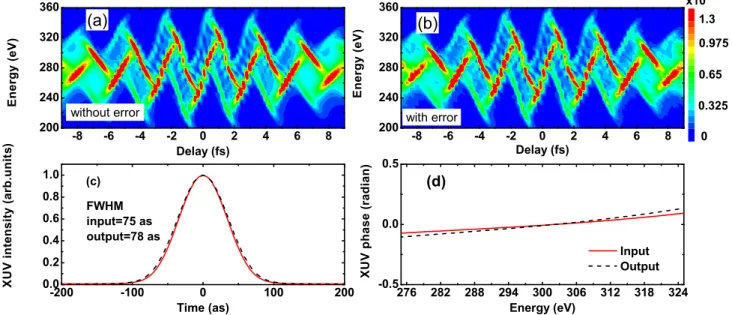
D. Sensitivity of phase retrieval to noise in spectrogram The examples given above use the spectrogram generated directly from solving the TDSE (Sec.III A) or calculated from the SFA (Secs.III BandIII C). When applying our method to real experimental data, there are inherent noises from the measurement. To test the sensitivity of the retrieved phase with respect to the noise, we artificially incorporate a random error up to 5% to each data point. In this test, the input parameters of the laser and the soft x-ray are the same as in Sec, III C. In Fig. 6, the top frames show the spectrogram with noise versus the one without the noise. At such a level of noise, the difference between two spectrograms is not visible. The bottom frames compare the intensity profile in the time domain and the phase in the energy domain, of the input soft-x-ray pulse with respect to that retrieved using PROBP. They agree very well. Thus the retrieved results are not sensitive to the noise in the spectrogram.
FIG. 6. Sensitivity of the PROBP method with respect to the noise in the spectrogram. Top frames show spectrogram calculated by using the SFA without any noise (left) and with a 5% random error at each point (right). Bottom frames compare the soft x-ray intensity in the time domain (left) and the spectral phase in the energy domain (right), between the input pulse (red solid line) and the output one (black dash line) retrieved by the PROBP, from the spectrogram with 5% random error.
E. Accurate carrier-envelope-phase retrieval of a long infrared pulse
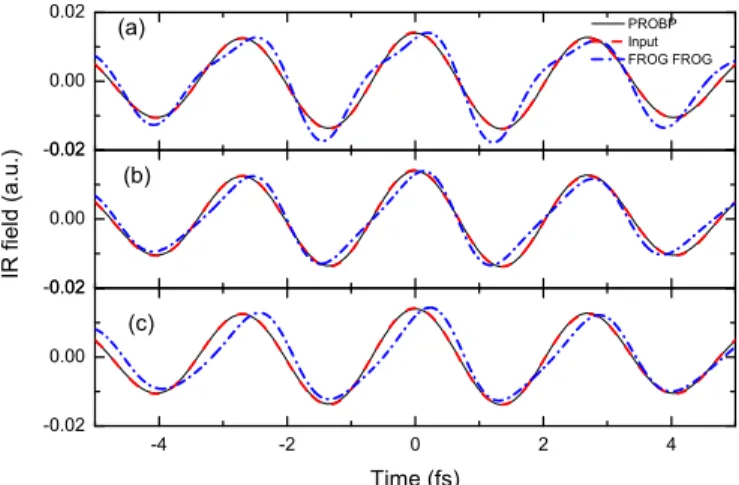
Both the FROG-CRAB and the PROBP allow the retrieval of the IR pulse as well as the XUV pulse. In this test, we examine how accurately the IR pulse is retrieved. It is well known that, for transform-limited few-cycle IR pulses, the carrier-envelope phase (CEP) will affect the nonlinear interaction of the laser pulse with matter. While the relative CEP between two few-cycle pulses can be measured from experiment, the absolute value of the CEP is difficult to determine. If single attosecond pulses are available in the laboratory, the IR field can also be retrieved in a streaking experiment with the methods of FROG-CRAB and of PROBP. To illustrate this capability, we took a long 20 fs IR laser pulse of 800 nm wavelength, 1013 W/cm2 in intensity and assume that it is transform-limited with a CEP ϕ0=0. In the retrieval, we assume that we do not know the IR pulse is transform limited, thus the IR is expressed in the form of Eq. (4) where the amplitude f(t) and the phase ϕI R(t) are unknown functions and each is expanded by B-spline basis functions. The SFA spectrograms were generated with this IR field and three different XUV pulses centered at 60 eV with a bandwidth of 23 eV. The XUV pulses have different chirped spectral phase so that their FWHM durations are 90, 130, and 230 as, respectively, compared with the 80 as transform-limited duration. Both FROG-CRAB and PROBP were applied to retrieve the IR field, and the results are plotted in Fig. 7. Clearly, the IR field is accurately retrieved by using PROBP but not by FROG-CRAB. The PROBP method reproduced a transform-limited IR field, with CEP=0, in all three cases, while the FROG-CRAB method retrieved a chirped pulse. Note that, in PROBP, the retrieved IR pulse is independent of the XUV pulses used as it should be. The error of the
FIG. 7. Retrieving an 800 nm, 20 fs input IR field (red dash lines) by FROG-CRAB (blue dash-dot lines) and by PROBP (black solid lines). The input IR pulse is transform limited with CEP=0. The streaking traces were generated by using three different XUV pulses with durations of (a) 90 as, (b) 130 as, and (c) 230 as, respectively. By using the PROBP method, the electric field of the IR is accurately retrieved for all three cases. The good agreement shows that the retrieved IR field is also transform limited with the CEP=0. On the other hand, when using FROG-CRAB, the retrieved IR pulses are different for the three cases and chirped.
retrieved IR field by the FROG-CRAB method was already noted in our previous study [30]. Such inaccuracy in the FROG-CRAB method would induce an error in the retrieved atomic dipole phase, as well as the retrieved “photoionization time delay,” which has been widely investigated in recent years on different targets. Unprecedented “accuracy” of the extracted “time delay” has often been quoted in these studies without accounting for the intrinsic error of the retrieval method [31].
F. Retrieving the phase of a broadband infrared pulse To generate intense single attosecond pulses, one way conceived by experimentalists is to start with a broadband IR pulse with a pulse duration of about one femtosecond. Such pulses span one or two octaves and can be obtained either with waveform synthesis of multicolor few-cycle pulses [26,27] or by the multiple-plate supercontinuum generation method [28]. Accurate characterization of such a broadband IR field is essential in order to understand how intense single attosecond pulses are generated. The photoelectron streaking method is an excellent method to characterize both the generated single attosecond pulses as well as the streaking broadband IR field. To test the method, we use an input IR pulse as given in Fig.8(a), as well as an attosecond pulse with central energy of 60 eV and width of 23 eV. The phase of the XUV is set to be unknown. To describe the broadband IR, we used the parametrization in the frequency domain, Eq. (5), where the spectral phase and amplitude are to be retrieved.
Using PROBP, the retrieved spectral phase and amplitude of the IR are shown in Figs.8(b)and8(c), respectively. They are in close agreement with the input ones. From the spectral amplitude, it can be seen that the broadband IR was synthesized from four waves with wavelengths of 2000, 1600, 1100, and 800 nm. The disagreement in the retrieved spectral phase at the low-energy and the high-energy wings is in the region where the spectral amplitude is very small. They contribute to small errors in the retrieved electric field in the temporal domain, as shown in Fig.8(a).
We tried the FROG-CRAB method but were unable to get converged results because the presence of mid-infrared wavelengths in the streaking field. This is similar to the failure of FROG-CRAB in Sec. III C. As another test, we used a waveform synthesized by four few-cycle IR pulses with wavelengths of 937, 610, 474, and 331 nm, covering almost three octaves, which was used in the experiment of Refs. [26,27]. The input pulse can be retrieved accurately by the PROBP method but not by FROG-CRAB, as demonstrated in Figs.8(d)–8(f). In this example, the error of FROG-CRAB lies in the spectral amplitude of the IR. The origin of such error is due to additional approximations in the FROG-CRAB algorithm when high-frequency components are present.
IV. SUMMARY
In summary, we have demonstrated that broadband sin-gle attosecond pulses can be accurately retrieved from the streaking spectra by using the retrieval algorithm PROBP. This method is applicable for characterizing soft-x-ray attosecond pulses covering the water window when mid-IR dressing laser
FIG. 8. Retrieving broadband laser pulses with PROBP. Panels (a) and (d) show the IR fields in the time domain. Panels (b) and (f) show the IR spectral phase. Panels (c) and (f) show the IR spectral amplitude. The red solid lines are the input field, the black dash lines are retrieved from the PROBP method and the blue dash-dot lines are retrieved from the FROG-CRAB method.
fields are used. Moreover, PROBP can retrieve the streaking IR or mid-IR field, including broadband laser pulses. In the meanwhile, this method can be applied to the typical experimental conditions that are identical to those used in the streaking measurements for narrow-band attosecond pulses where the FROG-CRAB method was used for phase retrieval. For such attosecond pulses the two methods agree reasonably well but PROBP in general is more accurate. Note that FROG-CRAB (and VTGPA) retrieve the XUV and IR fields from the time domain directly, while in PROBP we exploit the fact that the spectral amplitude of the XUV is readily
obtained from XUV photoionization measurements. In view of the insufficient accuracy of the FROG-CRAB retrieval method in general, the precision of the retrieved parameters should always be taken with caution.
ACKNOWLEDGMENTS
This research was supported in part by Chemical Sciences, Geosciences, and Biosciences Division, Office of Basic Energy Sciences, Office of Science, U.S. Department of Energy, under Grant No. DE-FG02-86ER13491.
[1] F. Krausz and M. Ivanov,Rev. Mod. Phys.81,163(2009). [2] E. Goulielmakiset al.,Science320,1614(2008).
[3] A. Jullien, T. Pfeifer, M. J. Abel, P. M. Nagel, M. J. Bell, D. M. Neumark, and S. R. Leone,Appl. Phys. B: Lasers Opt.93,433
(2008).
[4] I. J. Solaet al.,Nat. Phys.2,319(2006).
[5] H. Mashiko, S. Gilbertson, C. Li, S. D. Khan, M. M. Shakya, E. Moon, and Z. Chang,Phys. Rev. Lett.100,103906(2008). [6] K. T. Kim, C. Zhang, T. Ruchon, J. F. Hergott, T. Auguste,
D. M. Villeneuve, P. B. Corkum, and F. Quéré,Nat. Photonics
7,651(2013).
[7] T. Popmintchevet al.,Science336,1287(2012).
[8] M. C. Chen et al., Proc. Natl. Acad. Sci. USA 111, E2361
(2014).
[9] N. Ishii, K. Kaneshima, K. Kitano, T. Kanai, S. Watanabe, and J. Itatani,Nat. Commun.5,3331(2014).
[10] S. L. Cousin, F. Silva, S. Teichmann, M. Hemmer, B. Buades, and J. Biegert,Opt. Lett.39,5383(2014).
[11] C. Ding, W. Xiong, T. Fan, D. D. Hickstein, T. Popmintchev, X. Zhang, M. Walls, M. M. Murnane, and H. C. Kapteyn,Opt. Express22,6194(2014).
[12] K. Hong, C. Lai, J. P. Siqueira, P. Krogen, J. Moses, C. Chang, G. J. Stein, L. E. Zapata, and F. X. Kärtner,Opt. Lett.39,3145
[13] F. Silva, S. M. Teichmann, S. L. Cousin, M. Hemmer, and J. Biegert,Nat. Commun.6,6611(2015).
[14] J. Li, X. Ren, Y. Yin, Y. Cheng, E. Cunningham, Y. Wu, and Z. Chang, Appl. Phys. Lett. 108, 231102
(2016).
[15] S. Hädrich, J. Rothhardt, M. Krebs, S. Demmler, A. Klenke, A. Tünnermann, and J. Limpert,J. Phys. B: At., Mol. Opt. Phys.
49,172002(2016).
[16] J. Tate, T. Auguste, H. G. Muller, P. Salières, P. Agostini, and L. F. DiMauro,Phys. Rev. Lett.98,013901(2007).
[17] Y. Mairesseet al.,Science302,1540(2003).
[18] K. Zhao, Q. Zhang, M. Chini, Y. Wu, X. Wang, and Z. Chang,
Opt. Lett.37,3891(2012).
[19] Y. Mairesse and F. Quéré,Phys. Rev. A71,011401(2005). [20] J. Gagnon, E. Goulielmakis, and V. S. Yakovlev,Appl. Phys. B:
Lasers Opt.92,25(2008).
[21] V. S. Yakovlev, J. Gagnon, N. Karpowicz, and F. Krausz,Phys. Rev. Lett.105,073001(2010).
[22] M. Chini, S. Gilbertson, S. D. Khan, and Z. Chang,Opt. Express
18,13006(2010).
[23] H. Wei, A. T. Le, T. Morishita, C. Yu, and C. D. Lin,Phys. Rev. A91,023407(2015).
[24] P. D. Keathley, S. Bhardwaj, J. Moses, G. Laurent, and F. X. Kärtner,New J. Phys.18,073009(2016).
[25] H. Bachau, E. Cormier, P. Decleva, J. E. Hansen, and F. Martín,
Rep. Prog. Phys.64,1815(2001).
[26] O. Proninet al.,Nat. Commun.6,6988(2015). [27] M. Th. Hassanet al.,Nature (London)530,66(2016). [28] C. Lu, Y. Tsou, H. Chen, B. Chen, Y. Cheng, S. Yang, M. Chen,
C. Hsu, and A. H. Kung,Optica1,400(2014).
[29] X. M. Tong and C. D. Lin,J. Phys. B: At., Mol. Opt. Phys.38,
2593(2005).
[30] H. Wei, T. Morishita, and C. D. Lin,Phys. Rev. A93,053412
(2016).
[31] R. Pazourek, S. Nagele, and J. Burgdörfer,Rev. Mod. Phys.87,