Scheduling and Prefetching in Hadoop with Block Access Pattern Awareness and Global Memory Sharing with Load Balancing Scheme

(1)

Computer Science and Engineering: Theses,

Dissertations, and Student Research Computer Science and Engineering, Department of

Summer 6-10-2019

Scheduling and Prefetching in Hadoop with Block

Access Pattern Awareness and Global Memory

Sharing with Load Balancing Scheme

Sai Suman

University of Nebraska - Lincoln, [email protected]

Follow this and additional works at:https://digitalcommons.unl.edu/computerscidiss

Part of theComputer Engineering Commons, and theComputer Sciences Commons

This Article is brought to you for free and open access by the Computer Science and Engineering, Department of at DigitalCommons@University of Nebraska - Lincoln. It has been accepted for inclusion in Computer Science and Engineering: Theses, Dissertations, and Student Research by an authorized administrator of DigitalCommons@University of Nebraska - Lincoln.

Suman, Sai, "Scheduling and Prefetching in Hadoop with Block Access Pattern Awareness and Global Memory Sharing with Load Balancing Scheme" (2019).Computer Science and Engineering: Theses, Dissertations, and Student Research. 171.

(2)

A THESIS

Presented to the Faculty of

The Graduate College at the University of Nebraska In Partial Fulfilment of Requirements

For the Degree of Master of Science

Major: Computer Science

Under the Supervision of Professor Ying Lu

Lincoln, Nebraska March, 2019

(3)

PATTERN AWARENESS AND GLOBAL MEMORY SHARING WITH LOAD BALANCING SCHEME

Sai Suman, M. S. University of Nebraska, 2019 Adviser: Ying Lu

Although several scheduling and prefetching algorithms have been proposed to improve data locality in Hadoop, there has not been much research to increase cluster performance by targeting the issue of data locality while considering the 1) cluster memory, 2) data access patterns and 3) real-time scheduling issues together.

Firstly, considering the data access patterns is crucial because the computation might access some portion of the data in the cluster only once while the rest could be accessed multiple times. Blindly retaining data in memory might eventually lead to ineffcient memory utilization.

Secondly, several studies found that the cluster memory goes highly underutilized, leaving much room that can be leveraged for storing input data for future tasks. Leveraging the aforementioned memory underutilization in the clusters is important since the nodes are usually equipped with large amounts of memory.

Thirdly, enabling a prefetching mechanism to retain popular blocks in memory could eventually lead to memory shortage, we thus present two cache eviction al-gorithms to evict the data that will not be accessed frequently. Furthermore, the caching mechanism could potentially lead to unbalanced utilization of memory in a cluster’s nodes, so we present a mechanism for balancing the memory loads across the cluster such that the utlization of the memory on all nodes is uniform and no node’s

(4)

WordCount benchmark. We present the results showing that our framework causes no interference with the existing Hadoop ecosystem. Our experiments show that the framework achieves improved job completion times, higher memory utilization, higher locality placement of tasks and also better overall system performance.

(5)

COPYRIGHT c

(6)

terns and Memory Locality Problem in Distributed Systems research area. I am very grateful to her for the immense amount of time that she dedicated for supervision, for her patience, continual support, motivation and knowledge leading me into the appropriate methods and techniques needed in this work. Her knowledge and enor-mous support has been the key to all my work, and for that I am very grateful! Next, I would like to thank my committee members Dr.Lisong Xu and Dr.Hongefng Yu, thank you for devoting your valuable time to improve the thesis.

I would like to thank all my graduate student colleagues who helped me by proof-reading the write up of this thesis and for their continuous support. Next, I would like to thank other professors who I have worked closely over the past couple of years for their continuous guidance and for motivating me in my graduate career when the times were seemingly tough. Finally and most importantly, I must express my very profound gratitude to my family members, and friends for providing me with unfailing support and continuous encouragement throughout my years of study and through the process of researching and writing this thesis. This accomplishment would not have been possible without them, especially my parents who have supported me by showing me the right path whenever I tend to veer off. Thank you.

(7)

List of Figures

2.1 Breakdown of a MapReduce Job . . . 10

2.2 YARN Resource Negotiation and Application Execution Flow . . . 12

2.3 HDFS Architecture . . . 14

4.1 An Example Scenario of Task Assignment Based on Memory Locality . 26 6.1 GutenbergSmall Workload . . . 45 6.2 GutenbergLarge Workload . . . 45 6.3 BlogCorpusTogether . . . 46 6.4 BlogCorpus1 . . . 46 6.5 BlogCorpus2 . . . 46 6.6 4GBWorkload . . . 46 6.7 10GBWorkload . . . 46 6.8 20GBWorkload . . . 47 6.9 GutenbergLarge Workload . . . 51 6.10 GutenbergSmallA Workload . . . 52 6.11 GutenbergSmallB Workload . . . 52 6.12 BlogCorpus1 Workload . . . 52 6.13 BlogCorpus2 Workload . . . 53 6.14 BlogCorpusCombined Workload . . . 53

(10)

(11)

List of Tables

6.2 Configuration of GutenbergSmall workload overall . . . 40

6.1 Individual configurations of files in GutenbergSmall workload . . . 41

6.3 Configuration of GutenbergLarge workload . . . 41

6.4 Configurations of files in Blog Authorship Corpus workload . . . 42

6.5 Configuration of the Blog Authorship Corpus workload overall . . . 42

6.6 Configurations of the three larger workloads . . . 42

6.7 Configurations of nodes in the cluster . . . 44

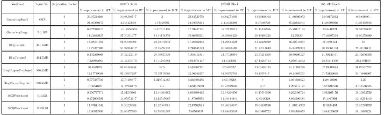
6.8 MT- Map Execution Time; RT- Reduce Execution Time; JCT- Job Com-pletion Time . . . 47

(12)

(13)

Chapter 1 Introduction

In recent years, as devices from sensor networks to corporate enterprises, vehicles and embedded devices generate increasing amount of information, large-scale distributed systems, have become a major platform for processing information for back end ap-plications, which perform sophisticated analytics to make optimization decisions for real world problems. This can be evidenced by the fact that big data analytics tools like MapReduce[1] and Apache Spark[2] have been widely adopted by both the indus-try and research community for performing sophisticated data processing, analytics, storage and mining. Apache Hadoop[19] is one of the most widely used open source frameworks for real time storage and processing of large data on huge clusters.

Many data intensive computing applications are characterized by the fact that they operate on time-sensitive data and involve large computational workloads while sharing resources with best-effort latency sensitive applications. The existing state-of-the-art frameworks have not yet been able to meet the requirements set by these properties to guarantee real-time performance metrics like end-end latency, through-put, and individual application deadlines.

(14)

lean-process complex queries over large amount of static data[24]. Hadoop is fully open source, is continuously evolving and dominates other batch processing system with its widespread usage in both industry and academic research.

A key challenge in Hadoop framework is increasing the memory utilization to improve the overall performance. HDFS[20], the underlying distributed file storage system of Hadoop, stores the data distributed across all the nodes of the cluster. Distributed processing frameworks schedule jobs (or) applications across all nodes of a cluster to maximize the utilization. Underlying schedulers in these frameworks prefer scheduling individual tasks in the nodes that contain their input data to reduce the remote I/O data copy operations which would otherwise cause data transmission overhead. In other words, placing computation near the data, is deemed important because both the network I/O and data I/O could become bottlenecks.

Another challenge in Hadoop has been the efficient usage of the network band-width to maintain performance of the cluster as well as provide high data throughput. The network bandwidth speeds have increased so much in recent years but it can still be a bottleneck slowing down the performance[6] and can lead to excessive resource usage in the cluster. Many workloads that run on Hadoop can arrive with a require-ment of high data rate so that their deadlines are met. The contention for network bandwidth becomes difficult to handle when there are such applications requiring high throughput as well as low latency[27]. Moreover, since the application has to compete with other applications in the transfer of data between nodes, network band-width becomes a big contention issue[28]. One option to address the network being

(15)

the bottleneck when the cluster runs workloads that have high data rate requirement is to use network equipment with sizeable buffers which can handle the network con-gestion issues. Obviously, this solution is not always feasible as it comes with a high price tag and requires significant rework of the existing infrastructure.

Increasing amount of evidence shows that as the number of jobs in the cluster increases, disk and network I/O bandwidth can be a huge limiting factor for achieving desired performance[11]. In practice, the cluster resources are shared between several users that run heterogeneous applications that contend for cluster’s resources. This makes it very difficult for the scheduler to assign tasks to nodes that store its input data[21]. Intuitively, the scheduler will always try to place a task in a node with the data. In some cases, the scheduler might even wait for a period of time so that the node with the data might become available in a future point of time. If the scheduler does not find a node on the clutser with the data required for the task, it will then try to place the task on a node where the data is in the same rack. If the scheduler is unsuccessful again, it will have to place the task in a node far away from the data. This mechanism induces delay(s) i) while the scheduler tries to place the task near the data and ii) also when the scheduler places the task in a node without the required data. The latter delay is due to remote data access which requires the copy of the required data for the task from a remote node where the data is physically located. This is why achieving the desired data input locality for an application is of paramount importance so as to address this latency as much as possible[4].

One mechanism that could help in addressing the aforementioned delays and bot-tlenecks is the data prefetching mechanism, which is a big part of my work in this thesis. Data prefetching is a data access technique that retrieves the required data for future tasks into the nodes.

(16)

that this memory overprovisioning leads to its high underutilization. Another study done on Facebook cluster data shows that the median memory utilization is around only 10%, leaving much room that can be leveraged for storing input data for future tasks[12]. Many studies show that inefficient memory usage is one of the major rea-sons for degraded performance of the cluster. Since the nodes in clusters are usually equipped with large amounts of memory, which is often underutilized, prefetching the required data for future tasks into the memory has a potential to increase the performance of the applications by reducing the effects of bottlenecks due to data I/O and Network I/O.

Although several scheduling, prefetching algorithms to hide the access delay have been proposed to improve data locality in Hadoop, there has not been much research targeting both data locality, data access patterns and real-time scheduling issues to-gether. Some research efforts have focused on inter-block and intra-block prefetching schemes in an earlier version of MapReduce framework to improve data locality for map tasks[13]. For example, Tao Gu et al. proposed a prefetching framework for MapReduce in heterogeneous environments[17]. However, these studies do not con-sider the data access patterns across the cluster while prefetching and caching the required data for tasks.

Considering the data access patterns is crucial because the computation might access some portion of the data in the cluster only once while the rest could be accessed multiple times. Blindly retaining data in the memory might eventually lead to ineffcient utilization of the memory. Work done in [14] shows that 2.5% of the

(17)

files are accessed more than 10 times, 1.5% of files are accessed more than 3 times concurrently while 90% of the files are not accessed by more than one task at a time. It is also known that data popularity also changes over time and can be leveraged to predict the future access patterns. This information can be used to cache popular data blocks in the memory, to be used by the later tasks or applications. Examples of data that is accessed more frequently during computation are hash tables, data structures and objects etc. So retaining the data blocks that are accessed more could lead to increase in performance of the cluster and help the jobs and applications maintain their real-time constraints. This is due to the fact that it avoids the data and network I/O delay as there is potentially no remote data access in this case. The Namenode [30], the centralized server of the HDFS, due to its awareness of the data block accesses from the blockreports from the nodes, handles the responsibilty of marking some blocks popular across the cluster, not just a node. This makes the maintenace of metadata of popular blocks a part of the already existing bookkeeping system about the blocks in the cluster’s nodes. Keeping in mind that the memory on the cluster nodes could get overutilized due to prefetching mechanism and the retention of popular blocks, we need an efficient data block replacement mechanism for the data in the node’s memory such that the data not accessed frequently should be a prime candidate for eviction.

Ananthanarayanam, Ganesh et al.[14] and Abad, Cristina L. et al.[15] developed data replication algorithms that exploit the data access patterns to help the underly-ing scheduler to make schedulunderly-ing decisions with data locality decisions. Another work by Ibrahim, Shadi, et al. [16] proposed a sheduling algorithm with the main focus to increase the data locality by reducing the amount of unbalanced execution of tasks across nodes and by predicting the next appropriate task to be placed. Even though these studies focus on load balancing and distribution of data across the cluster, we

(18)

couple of decades that having a centralized scheduler that migrates the threads across different workers leads to less frequent migration compared to a case where the workers themselves take responsibilty of actively sharing the workload [25], . This mechanism has been termed as "work stealing" and has been thoroughly studied in several studies and has been applied to "steal" resources [26], workloads[25] etc. These studies repeatedly found that the stealing mechanism leads to better load balancing and higher resource utilization.

Due to the presence of centralized scheduler in the form of Resource Manager in the Hadoop YARN system[18], the same logic could be easily extended for balancing the memory loads across the nodes in the cluster such that the utlization of the memory on all the nodes is uniform and no node’s memory is overutilized due to the prefetching mechanism. Since this thesis proposes a prefetching mechanism that is data access pattern aware, the load balancing mechanism becomes crucial so that popular blocks in a node are still retained in the cluster by migration if possible, instead of evicting them when the node’s memory is close to being fully utilized. Even after migration to a different node, this mechanism still retains the usefulness offered from retaining popular blocks in the memory because the blocks were deemed popular across the cluster, not just within the original node.

We propose a framework for locality aware real-time scheduling system on Hadoop that focuses on increasing memory utilization and achieving improved job completion time and system performance. The main contributions of our framework are :

(19)

1. Leverage data access patterns across the cluster and use the metrics to make caching decsions and improve the data locality

2. Make the prefetching, caching and load balancing mechanisms centrally coordi-nated so that the individual nodes are not "actively" participating

3. Leverage the memory locality awareness for better scheduling decisions by the Hadoop YARN system

4. Make the caching mechanism globally managed and accessible throughout the cluster

5. Replacement schemes in the cache that respect the popularity history of the blocks

6. Centrally coordinated load balance mechanism for cached data to maintain uniform distribution acorss the cluster

7. Since applications run in waves of tasks[10], we try to improve the data locality for entire waves of tasks to speed up their execution

8. We evaluate our framework on a real cluster

Rest of the thesis is structured as follows. Chapter 2 presents the background and re-lated work, Chapter 3 presents the design and implementation, Chapter 4 presents the theoretical analysis, Chapter 5 presents the experimental methodology and Chapter 6 presents our results.

(20)

Chapter 2 Background

Hadoop (Highly Archived Distributed Object Oriented Programming) is a distributed processing framework that has been designed to process huge amounts of data spread across, potentially, hundreds to thousands of nodes in a cluster environment. Hadoop is released as an open source project in Java technology forming a part of the Apache Software Foundation umbrella, which is a non-profit open software foundation that has maintained a very important role in the distrubuted processing field [29]. Hadoop handles and allows processing of multitude of data types like audio, video, text, records, queries and even unstructured data. An important property of Hadoop is that the data is distributed across hundreds or thousands of nodes in the cluster while concurrently running computation in close proximity to their required data.

2.1 Architecture of Hadoop

Hadoop has three main components or layers as we call them in this thesis. i) Hadoop Distributed File System (HDFS), which is a distributed file system designed keeping in mind scalability, data availability ii)Hadoop YARN, a resource management and

(21)

scheduling component and, iii) Hadoop MapReduce a parallel programming paradigm for running applications to process large amounts of data in the cluster.

2.2 MapReduce

Hadoop MapReduce is data-driven parallel processing paradigm of Hadoop that runs on top of Hadoop YARN. MapReduce makes the parallelization of processing trans-parent to the application programmers and helps them focus on writing the data processing applications. MapReduce layer is where the programmer writes their ap-plication and where the apap-plication (or Job) is "run".

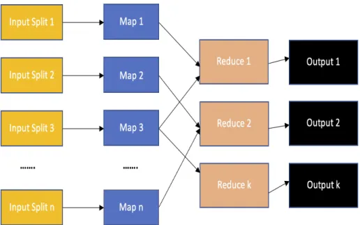
The core of MapReduce is splitting up the computation i.e, the application/Job into two phases, each containing different types of tasks. These phases are called i)Map, ii)Shuffle, iii)Reduce phases. Across these phases, there are two types of tasks in MapReduce: map tasks and reduce tasks. At first, the original input data is partitioned into several splits, with each split the size of several blocks. The map tasks in map phase consume one split each from the original input data required by the application parallely and processes the data as intended by the application. After processing the data, map tasks produce "intermediate" results, which contain a collection of key/value pairs. This intermediate data produced by map tasks is sorted according to their key values. The sorted collection of key/value pairs undergo shuffling, where the data is sent to appropriate reduce tasks as inputs. The reduce tasks then sort the received key/pairs from several different map tasks according to their key values, once this is done the final output data is written to the underlying distributed file system, HDFS. This process is visulaized in Figure 2.1.

(22)

Figure 2.1: Breakdown of a MapReduce Job

The main component of MapReduce is a per-application Application Master (AM) that interacts with the YARN component for resource negotiation and runs the tasks.

2.3 YARN

Hadoop YARN (Yet Another Resource Negotiator) forms the resource management and job scheduling layer of the Hadoop architecture. YARN was introduced in Hadoop version 2.0 as a way to take off the resource managament and scheduling duties from the MapReduce into a separate component. This was done to improve the scalability of the Hadoop framework without over-burdening the MapReduce component with resource management and scheduling duties. The main changes that YARN brought into Hadoop environement are that it i) now delegates the scheduling responsibili-ties to a per-application component in the form of MapReduce’s Application Master (AM), ii) provides dynamic allocation of cluster resources to the applications running in the cluster. This is a move away from the static allocation of resources to the

(23)

ap-plications that was implemented during Hadoop version 1. Dynamic allocation brings better cluster utilization due to its intrinsic ability to adjust the resources allocated to applications on-the-go.

The main components of YARN are the per-cluster Resource Manager (RM) and the per-node Node Manager (NM). Resource Manager runs on a single dedicated node in the cluster and takes the responsibility of management and allocation of cluster resources among the applications running in the cluster.

Resource Manager (RM) runs several components, the most important ones among them are the YARN Scheduler, Application Master Launcher and the Application Master Service (also known as Application Manager Service). YARN Scheduler is an abstract service that receives heartbeats from the nodes and also allocates requested resources such as memory, CPU, disk, network etc., to the applications running in the cluster. The resource allocation provided by the scheduler is constrained by the current cluster metrics like available capacities, waiting queues etc. YARN supports several types of schedulers like FIFO (first-in-first-out), capacity and delay schedulers. The scheduler allocates resources to the applications in the form of containers. A container is a collection of resources like CPU, memory, disk, network etc., that is required to run the application. Application Master Launcher is a thread running in RM that receives requests for new applications and then launches a corresponding application master (part of MapReduce component). Application Master Service is a thread that receives RPCs (remote procedure calls) from the application’s application master (AM) and forwards their resource allocation requests to the YARN scheduler. Node Manager is daemon that runs in all slave nodes of the cluster and acts as a slave to the Resource Manager, which is the master. The main duty of Node Manager (NM) is to monitor the resources on its host node by communicating with the AM(s) running on the host node and the containers allocated to the AM (and hence the

(24)

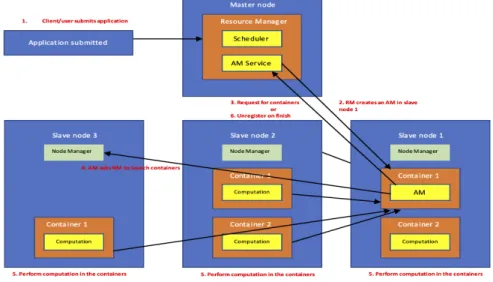
Figure 2.2: YARN Resource Negotiation and Application Execution Flow The flow in Figure 2.2 could be explained as follows: The client or user writes an application and submits it to the RM. The AM launcher in RM launches an AM for the application in its own container in some node. The AM negotiates resources with the RM and once they are granted, AM launches the allocated containers in other slave nodes by communicating with the NM residing in those nodes. The launched containers perform the task’s computation, orchestrated by the AM. NM monitors the resource usage of the containers in its node and keeps in touch with the RM via periodic heartbeats. Once computation is finished i.e., the application has finished its execution then the AM unregisters with RM and asks to deallocate the containers granted to it.

(25)

2.4 HDFS

HDFS is the main underlying open-source distributed file system of Hadoop providing scalablity, reliability, fault tolerance and availability of data. HDFS splits and distr-butes large amounts of data across thousands of machines in the cluster. To handle failure or corruption issues of data in a machine, HDFS also replicates all data in the cluster in several machines (default is 3 machines). Similar to YARN, HDFS follows a Master-Slave architecture. There are two major components in HDFS: i) NameNode and, ii)per-node DataNode.

There can be multiple NameNodes in an HDFS cluster, one per namespace. Na-meNode acts as a master that manages the data stored across the cluster and handles its access by the applications. NameNode manages a namespace, which is a hierar-chical structure of a filesystem and directories. NameNode orchestrates the access to the files in its namespace from the applications running in the cluster. NameNode also maintains a large hashmap in its memory that contains a mapping between each DataNode under it and the HDFS blocks stored on that DataNode. A HDFS block is simply a chunk of data of certain size, e.g. 64MB. NameNode instructs DataNodes to create, replicate, delete, copy and transfer the blocks. HDFS provides the ability to maintain a secondary NameNode for the same namespace that will replace the orginal NameNode in case of a failure.

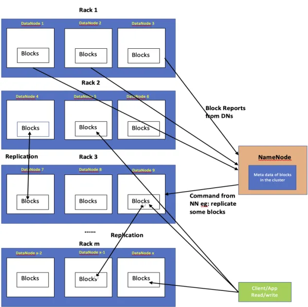
DataNodes are the slaves nodes that report to exactly one NameNode via Block-Reports (Similar to a heartbeat from Node Manager to RM in case of YARN). In each report, they provide the list of blocks and their metadata to the NameNode. The NameNode updates the metadata of the blocks using information provided from all DataNodes under it. DataNodes also receive commands from the NameNode to manipulate the blocks being hosted in them. Figure 2.3 illustrates the architecture

(26)

Figure 2.3: HDFS Architecture

Figure 2.3 illustrates an HDFS cluster with one NameNode, x Datanodes and m

racks. Note that a rack in HDFS is a set of nodes in the cluster that are connected to the same network switch.

(27)

Chapter 3 Literature Review

For the literature review, we examine the roles of locality and memory utilization on the cluster performance and on the individual application’s performance. We then consider some of the research work related to the methods aimed at improving data locality and memory utilization for the jobs in the cluster along with the methods aimed at load balancing and scheduling that form the part of such methods. Finally, we discuss the drawbacks of these research efforts.

It has been established in existing work that launching a task on a node that does not contain input data i.e., launching a remote task is inefficient because that node has to first fetch the task’s required input data from the origin, i.e., from the node conatining that data. This adds an access delay that will increase the task comple-tion time and therefore affects the system performance. In fact, data locality problem is one of the most studied issues in the field of distributed processing systems. As the number of applications running in the cluster increases, disk and network I/O bandwidth become bottleneck for achieving the desired cluster performance[11]. Ad-ditionally, the cluster runs numerous heteregenous applications from several hundreds of users and consequently all of them compete for the allocation of nodes so that they

(28)

easy task for the underlying scheduler [21]. To compensate for this, the native hadoop ecosystem uses delay scheduling mechanism which tries to improve data locality by first requesting to lauch tasks on nodes with input data and then wait for a certain amount of time hoping that the nodes would become available so that the task(s) could be launched on them [4]. Another well-known scheduler Quincy [35] proposed by Isard, M. et al. tries to address the data localilty issue by modelling it into a classic min-cost flow problem in a directed graph. There are several such schedulers that were studied which we cannot list due to space constraints. One major issue with these approaches is that if the scheduler does not find a task with local data on that node[31], a node maybe skipped by the scheduler for all the applications in the scheduler’s queue that are waiting for their tasks to be scheduled. This issue will have an affect on the scheduler’s performance and hence the application’s execution time, the system performance over all and may also lead to underutlization of the cluster’s resources. Another option provided by native hadoop ecosystem is FIFO scheduling system which schedules a task which is picked from a head-of-line application residing in a first-in-first-out queue of applications and launched on any node with data closest to that node. Although this mechanism prioritizes nodes with data on them, it does not make any effort in improving the data locality and hence it doesn’t make any promise on increasing the throughput and guarantees almost no locality.

An early work by He, C., et al. [38] in 2011 proposed a scheduling algorithm called Matchmaking to improve a task’s locality by prioritizing launching tasks on nodes with data on them while also reducing the wait time induced by the delayed

(29)

schedul-ing required for locality mechanism by settschedul-ing the waitschedul-ing threshold to be exactly one heartbeat interval. Ibrahim, S., et al. [16] proposed Maestro, a replica-aware schedul-ing algorithm for mapreduce system that aims at improvschedul-ing the locality of map tasks by keeping track of data block’s locations along with its replicas’ locations as well as the number of blocks on each node in the cluster. Maestro uses this information to schedule map tasks on nodes with the required data that causes the least amount of impact on other map tasks’ that are running on nodes which also host their data.

An important aspect of our work is effectively utilizing the data access patterns for improving data locality. There have been some studies done that have focused on looking at the data access patterns during the run time of the cluster and using that information to improve data locality for the future tasks. Data access patterns provide key information about which portions of the data distributed across the nodes in the cluster is only accessed once and which portions are accessed multiple times over a period of time. So retaining the data blocks that are accessed more could lead to increase in performance of the cluster and help the jobs and applications maintain their real-time constraints. This is due to the fact that it avoids the data and network I/O delay as there is potentially no remote data access in this case. In their study[14], Ananthanarayanan, Ganesh, et al. noted that 2.5% of the files are accessed more than 10 times, 1.5% of files are accessed more than 3 times concurrently while 90% of the files are not accessed by more than one task at a time. In the same study, they proposed Scarlett algorithm which leverages the popularity of the data blocks in HDFS by replicating the popular data blocks to address the bottleneck issues caused by hotspots. Another work by Palanisamy et al. [34] proposed Purlieus, a mapreduce resource allocation algorithm that aims at improving data locality among tasks while reducing the network overhead required for the remote data transfer. Purliues places the data on nodes that will run the task that require that data or at least place the

(30)

the data access patterns, their replication schemes are not run-time and the data needs to be replicated ahead of the application’s scheduling. Additionally, these studies do not make an effort to make the popular data accessible to other nodes across the cluster and they do not consider the fact that popularity of data is ever changing. It is important to note that data access patterns for any piece of data is constantly changing as newer applications are being added to the cluster and as the existign applications are making progress continuously. Since it is known that data popularity also changes over time and can be leveraged to predict the future access patterns. This information can be used to cache popular data blocks in the memory, to be used by the later tasks or applications. Examples of data that is accessed more frequently during computation are hash tables, data structures and objects etc.

Choi D, et al. [37] proposed a task scheduling algorithm that categorizes the tasks based on the the location of data blocks in their input splits and then sequentially launching tasks on nodes according to their priority that was calculated based on data locality of their input splits. The main contribution of this work is to reduce the performance degradation caused by copy of the data blocks in the task’s input split that are spread across several nodes. Zhang, X. et al. [39] proposed a next-k-node scheduling mechanism that calculates the probability for each task to be launched on a node such that the tasks with input data on the next k nodes have lower probabilties than other tasks. The scheduler then launches a task on a node that has its input data on that node. If it does not find such tasks for that node, it launches a task with highest probability on that node. In 2016, Wang et al. [31] proposed a task

(31)

scheduling algorithm that aims at improving data locality by considering a tade off between data locality for a task and the consequent load balancing. Although the study does a good job of considering the load balancing aspect involved to achieve the desired data locality, the limitation of the study is that it only addresses the optimization of load balancing from a network perspective but it does not address the issue of improving data locality itself by considering the data access patterns.

One mechanism that has been studied for quite some time is the idea of data prefetching, in which the required data is fetched to the node in advance where the task is to be executed. This idea is been aimed at improving data locality as well as reducing delays in the task’s execution caused by data copy over the network and thereby reducing the application’s execution time while improving performance. Seo, S. et al. [13] proposed HPMR, a prefetching and preshuffling mechanism for the earlier version of mapreduce system (when YARN did not exist yet). The prefetching mechanism prefetches an input split or data blocks for both map and reduce tasks. The preshuffling mechanism predicts where the reduce task might be placed after the map task finishes and based on this prediction it tries to increase the amount of data that is shuffled over the network in advance. Another work done by Tao Gu et al. [17] proposed a prefetching framework that models the problem as a form of producer-consumer problem, where the task running on a node without its input data on that node triggers a prefetch mechanism that prefetches data in a buffer from one end while the task processes the data from the other end of the same buffer. The limits of these two studies are that they do not aim at reducing the amount of tasks that are remote i.e., do not have required data on their nodes as they do not exploit the data access patterns. Additionally, they do not consider the data copy delay for prefetching the first chunks of input data.

(32)

application/job’s duration is spent on data copy operations. The study also found that the median and 95th percentile utilization of the cluster memory falls at 10% and 42% respectively. Sun, M. et al. [12] proposed a prefetching based scheduler for mapreduce system called HPSO which aimed at improving memory locality in the cluster. HPSO relied on the fact that prefetching accuracy improves the performance of the system. HPSO predicts which tasks will be assigned to which nodes and then uses this information to prefetch the data required by the task into the node’s memory thereby effectively overlapping the data transfer delay with the computation and thus hiding the delay from data transfer. However, a limitation of this work is that once the input data is prefetched and then cached into a node, there is no discussion on what happens to this data after the task is done processing on that data. This drawback also exists for the studies [13] and [17] that were mentioned in the previous paragraph. Also, HPSO and the aforementioned studies do not make any effort to consider the memory utilization imbalances caused by prefetching mechanism and neither do they consider any data retention or load balancing schemes for the prefetched and already processed data residing in the node memory of the cluster.

There were some studies that introduced a centrally coordinated shared memory system that exploits the cluster memory’s underutilization. One such work was done by Hwang, J. et al. [9], where they presented that most clusters overprovision their memory so that they can handle unpredictable bursty workloads that might occur in the future. Their study showed that 50% of the nodes in their cluster consisting of 50 nodes that have at least 30% of memory being underutilized as a consequence

(33)

of memory overprovisioning. Several other studies such as Ananthanarayan et al. [10], which is noted in this section, showed that overprovisioning the cluster memory leads to its high underutilization. In order to exploit this memory underutilization, Hwang, J. et al. proposed the Mortar framework, which runs a hypervisor process that repurposes the underutilized sections of memory in the cluster for storing task related data that is generated during run time. This run time data is essentially a prefetched data that can be an input for either a single task running on a node or for the entire application distributed across several nodes managed by a separate protocol. The nodes can freely add any spare memory to the shared memory managed by the hypervisor process which coordinates its usage for the entire cluster for storing prefetched data. The hypervisor can evict data from the shared memory if a node gets constrained in its memory usage. When it comes to exploiting the underutilization of memory in the cluster, the approach taken by this work is related to the approach taken in our thesis where we introduce a centrally coordinated process that manages the free memory as well, albeit our central process has added several functionalities with two notable functionalities being that our process leverages data access patterns to decide which data to cache and it actively manages which node has how much free memory instead of letting each individual nodes add the free memory.

There are a couple of recent works done in 2018 that are more closely aligned to the load balancing aspect employed in our work in this thesis that aims at balancing and maintaining a uniform utilization of memory across the nodes in the cluster. Load balancing aspect for maintaining uniform utilization of memory across the nodes in the entire cluster is important so as to not let any of the nodes go overutilized thereby affecting the cluster performance and to avoid hotspots.

Li, C. et al. [36] proposed a two mechanisms, one aimed at improving data locality by data migration or prefetching and the second aimed at determinging popular files

(34)

the task is executed. The work also presents a file synchronization mechanism which syncs only popular files between subcloud environments. The major drawback of this work is that they only consider the data access patterns for syncing files between different subcloud environments. The nodes within the subcloud i.e., nodes within a single (large) cluster system do not have direct access to the popular data and hence the effect of their file synchronization mechanism in improving the performance of the nodes within one single large cluster system is lacking. Additionally, although this work considers the data access patterns of the files, they do not consider the data access patterns of data at the block level. Finally, these two studies do not address the issue of what should be done to the prefetched data. This aspect is important to avoid imbalances in memory utilization. We need an efficient centrally coordinated data block eviction/replacement mechanism for the data in a node’s memory such that the data not accessed frequently should be a prime candidate for eviction thereby retaining more frequently accessed data. Our work in this thesis includes such a data eviction scheme.

As you can see there are several scheduling and prefetching algorithms focused on improving data locality and hence the system performance, there has not been much research that addresses data locality, data access patterns and real-time scheduling and load balancing issues together. To the best of our knowledge, our work is the first one that considers addressing these issues in a single framework and we propose that exploiting these properties together offers more improvements in performance.

(35)

Chapter 4 Design

4.1 Introduction

When the Application Master (AM) is initialized in one of the nodes by the Resource Manager(RM), it has to request the containers in the nodes while considering which

nodes offer best locality for the application. For this, AM has to know which nodes have the required blocks stored in their local memory or disks. Maintaining this information of the local memory is not optimal and comes with a heavy cost because the local memory tends to change frequently. In the approach taken in this thesis, local memory in each node is divided into two portions: local cache and global cache. The most popular and young (which are newly created blocks) blocks are stored in the global cache while the local cache stores the blocks that are needed to run the tasks. Due to the nature of the blocks stored in the global cache, its content does not change as frequently as local cache’s and the information about the blocks in the global cache is maintained at the NameNode (NN) of the HDFS layer. The locality information of the blocks in the global cache is made available to application masters. This information can be used by an application master to make better locality decisions

(36)

the local memory. The variable APi, called application popularity, keeps track of

the number of accesses made to the blocki by this application. The APi variable is

uniquely maintained for a blocki across all nodes that this application master has

tasks running on them. For this reason, this variable is updated only once the appli-cation finishes. The variableGPi, called global popularity, keeps track of the number

of accesses made to blocki across the cluster. Additionally, a reference bitRi is

main-tained for each block and is set whenever the block is accessed. This reference bit is used to evict least recently accessed blocks from memory with the modified clock algorithm.

AM knows that it needs to request w number of containers for its application.

AM first requests locations of the needed blocks in the cluster from the NameNode. AM then receives a list of nodes with needed blocks in their global cache, disks and racks. After the AM knows about the blocks and their locations in the global cache from global cache image, AM then sends the list of nodes that it wants the containers to be assigned on to the scheduler that runs at the RM. But first AM needs to make decision about which nodes to request the containers on.

4.2 Containers Request Algorithm

The main goal of AM at this stage is to offer the highest locality possible so it needs to request containers on the nodes that provide the highest locality for the application. AM requests the containers on a list of nodes with data on them in their global caches

(37)

Algorithm 1

1: procedure Get_Locations

2: Input: List of blocks B that are needed by the Application

3: Output: Locations, which is the mapping between list of blocks to node global

cache/node disk

4: for each block Bi in B do

5: Add locations ofBi in Global_Cache_Image to Locations

6: Add locations ofBi in HDFS to Locations

7: Initialise the application popularity APi = 0

return Locations

or disks. The nodes with the highest number of needed blocks in their memory have the highest priority. Ties are broken with the highest number of needed blocks in the rack’s memories, the node’s disk and then the rack’s disks. First, nodes in the cluster are ranked according to their locality information stored in their respective node rank

N Rj for node Nj.

While considering the nodes to request containers on, first the nodes in the cluster are ranked according to their locality information stored in their respective node rank

N Rj for node Nj. Node rankN Rj of node Nj is represented as a vector of length 4 :

(a,b,c,d). a is the number of blocks of the application stored in node Nj’s memory.

Note that the local cache content is not known to the application master until it launches a container so a is the number of blocks in the node’s global cache only. b

is the number of blocks in global cache memory of nodes on the same rack asNj. cis

the number of blocks in the disk ofNj. dis the number of blocks in the disk of nodes

on the same rack as Nj. Note that a block is only considered once in calculating

a,b,c,d and its replicas are not counted.

Assuming that we have two nodes N1 and N2, N1 has a higher node rank than N2 i.e., (a1, b1, c1, d1) ≥ (a2, b2, c2, d2) if a1 > a2 or (a1 = a2 and b1 > b2) or (a1 = a2 and b1 = b2 and c1 > c2) or (a1 = a2 and b1 = b2 and c1 = c2 and d1 > d2) or (a1 = a2 and b1 = b2 and c1 = c2 and d1 = d2). AM must decide (N1, X1),

(38)

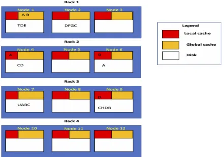
Figure 4.1: An Example Scenario of Task Assignment Based on Memory Locality

(N2, X2)...(Nj, Xj)...(Nk, Xk)where(Nj, Xj)denotes requestingXj number of

con-tainers on nodeNj.

Consider the cluster shown in Figure 1, the application has five tasks T1, T2, T3, T4, T5, each needing the blocks A, B, C, D, E respectively. Suppose for this job w is

3 so the application master requests three containers. The node ranks of the cluster are N R1 = (2,0,2,1), N R2 = (0,2,2,1), N R3 = (0,2,03), N R4 = (1,1,2,0), N R5 = (0,2,0,2), N R6 = (1,1,0,2),N R7 = (0,1,3,1),N R8 = (0,1,0,3), N R9 = (1,0,3,1), N R10 = (0,0,0,0), N R11 = (0,0,0,0), N R12 = (0,0,0,0) . AM adds N1 to the

request as it has the highest number of blocks in local memory and updates N R1 to

be (1,0,2,1). After that N4 becomes the node with the highest node rank. Similarly N6 is added to the request as the host of the final container.

After adding a container to the request, the node rank is updated by reducing the number of blocks in the memory by 1 if it is non zero. Otherwise we decrease the number of blocks in rack global cache, the number of blocks in local disk or the number of blocks in the rack’s disks by 1 whichever is the first to be found non zero.

(39)

Algorithm 2 Containers Request

1: procedure Request_Containers

2: Input: none

3: Output: List of containers to request 4: Calculate N Rj for all Ni in N

5: while request_size less than w do

6: Select Nj with the maximum node rank (a,b,c,d) i.e. the node Nj where

∀ k k6=j, we have N Rj ≥ N Rk 7: request.add(Nj,1) 8: UpdateNR(Nj) 9: 10: procedure _UpdateNR 11: Input: Current N Rj (aj, bj, cj, dj) 12: Output: Updated N Rj (aj, bj, cj, dj) 13: if thenaj 6= 0 14: aj -15: else If bj 6= 0 16: bj -17: else If cj 6= 0 18: cj -19: else 20: dj -21: return N Rj

4.3 Container Assignment Algorithm

After AM requests the containers from the RM, the scheduler at RM has to decide which application needs to be assigned which conatiners on the nodes of the cluster. Once the scheduler at RM receives the AM’s container request, it starts to make scheduling decisions to decide which nodes to allocate the containers on from the list of nodes received from AM in its request. The scheduler maintains i) a list of applications that sent container requests to it and are now waiting for containers and, ii) a list of nodes in the cluster that are available for placing containers on them.

Whenever a node becomes avaliable to be allocated a container(s) on (via node update message sent to the RM by the node), the scheduler needs to make the decision

(40)

The following are the steps involved in calculating block weight for a block. First, the related blocks of node j are divided into four categories : αj are the application’s

blocks in the local memory,βj are the application’s blocks in the global cache of nodes

located on the same rack,γj are the application’s blocks in the local disk of the node

and δj are the application’s blocks in the local disk of the nodes located on the same

rack.

An individual gain of processing a block on a node is either 10, 8, 4 or 2 depending on whether the block falls into αj, βj, γj or δj category respectively. Let τij be the

individual gain of processing block i in node j, then the relative gain of processing

blocki on node j is the ratio of the gain τij to the summation of individual gains of

all application’s blocks on node j. The block weight BWi can be calculated as the

summation of relative gains of processing block i on other nodes with containers. Block weight for block i is BWi = P

Nk←φ−Nj

τik/(10∗size(αk) + 8∗size(βk) + 4∗

size(γk) + 2∗size(δk))−8∗size((αk∩βk))−4∗size((αk∪βk)∩γk)−2∗size((αk∪

βk∪γk)∩δk), where size() gives the size of the set, φ represents all the nodes with

containers for the application.

In the above expression, the numerator τik represents the gain τ for processing

blocki on node k. If the block is in the local memory τik is 10, if the block is in rack

memory thenτik is 8, if the block is in node k’s disk thenτik is 4 and if the block is in

rack disk then τik is 2. The denominator represents summation of gain in processing

some "local" blocks on node k. The lower the ratio (also called relative gain), the less likely that block i will be picked to run on node k locally. Thus, a lower block weight

(41)

indicates that the block has a higher probability of being processed non locally if not being chosen to run on node j.

The block weight is calculated for all blocks in the current node and the nodes in the same rack. Once block weights for all blocks are calculated for the application, the average block weight for that applicaton is calculated. Similarly the scheduler proceeds to calculate the average Block Weights (BW) for each application on that node and puts the application-BW pair in a list. Once the scheduler calculates the average BWs of all the applications waiting for container(s) on this node, it picks the application with the lowest BW on that node and assigns the maximum possible containers for that application on the node. This ensures that we assign containers to the application on this node with its tasks having the highest probability of being processed non locally if not being granted containers on this node. Note that maxi-mum possible containers on a node is the minimaxi-mum of number of requested containers on the node by the application and the maximum allowed number of containers on the node. The latter depends on the cluster configuration and settings.

The following algorithm describes the container assignment process discussed above.

Algorithm 3 Container Assignment

1: procedure _{Container_Assignment}

2: Input: List of applications {application1...applicationk} waiting for

contain-ers on node Nj

3: Output: Containers granted to one application from the list

4: for each application applicatoni in the list {application1...applicationk} do

5: Calculate averageBWi for applicatoni

6: Application_BW_List.put(applicatoni, averageBWi)

7: while Nj can host more containersdo

8: Pick the application applicationl with lowest averageBW from

Application_BW_List

(42)

task dispatch decisions.

When the task begins processing the blocks during its execution phase, the block needs to be brought into local memory if it is not in the local memory already. If the number of blocks in the local memory is above the maximum threshold then some of the blocks need to be evicted. We denote Mj as the number of blocks in node Nj’s

local memory, Mmax is the maximum threshold of the local memory of a node. The

local cache eviction algorithm is called when a block needs to be fetched or prefetched and when Mj =Mmax.

Once a task is dispatched, a prefetch instruction is also called to fetch a block into nodeNj’s memory.

(43)

Algorithm 4 Task Execution 1: procedure Task Execution

2: Input: Node Nj

3: Pick the first block needed Bi

4: if the block not in Nj’s memorythen

5: Call Local_Cache_Eviction(Nj) if Mj =Mmax

6: FetchBi into Nj’s local cache, Mj++

7: Process block Bi in node Nj and make reference bit Ri = 1

8: APi++

9: N P[i, j] ++ 10: Prefetch(Nj)

11: procedure _Prefetch

12: Input: Nj

13: Output: One block that is chosen to be prefetched into node Nj’s local cache

14: U ← list of blocks needed by AM that are not in local cache of nodes where

AM has the container(s)

15: if U not nullthen

16: Select first block p from U

17: Remove p from U

18: if Mj == Mmax then

19: Local_Cache_Eviction(Nj)

20: InstructNj to fetch block p

(44)

to j

4: N Ptotal+ =N Pi

5: N Pavg =N Ptotal/Mj

6: Eflag = 0

7: for each blockBi whereN Pi ≤N Pavg do

8: if Ri equals 0 then 9: Evict Bi 10: Mj -11: Eflag = 1 12: break 13: Else 14: Ri ← 0 15: If Eflag = 0 go to 7

The above algorithm describes the local cache eviction strategy. If there is no space in the local cache for a new block then an unpopular block that has not been recently used is evicted. We categorize the unpopular blocks as the blocks whose node popu-larity is below average value. The average node popupopu-larity of the blocks in the node is calculated at line 4 and is denoted by N Pavg. Then an unpopular block is evicted

by running the clock algorithm, otherwise known as second chance algorithm defined from lines 5 to 15. Note that the reference bit Ri is updated in line 7 in procedure

Task_Execution in algorithm 4.

4.6 Global Cache Eviction and Load Balancing

After AM is done executing all the tasks in the application, it has to decide if the blocks processed by it should be moved to the global cache. Since the global cache

(45)

maintains young and popular blocks, AM needs to check if the blocks are both young and popular. A block is considered popular if its global popularity GP is above the global average popularity GPavg. First, the global popularity of blocks should be

updated by adding the number of accesses made to the blocks by the application executed by AM, this is done by a call to the procedure UpdateGlobal. Then all the blocks whose global popularity is above global average are moved to global cache. If none of them are young and popular then the blocks are just left in the local cache. The algorithm Finish describes this process and it is executed when AM has finished executing the application.

Algorithm 6 Finish 1: procedure _Finish

2: Create a list containing all blocks in the local memory of nodes with AM’s

containers and their respective application popularity AP called APlist

3: GPlist ←UpdateGlobal(APlist)

4: for each block Bi do

5:

6: if GPi > GPavg && creation time of Bi <24 hours then

7: MoveToGlobal(Bi)

8: procedure _UpdateGlobal

9: Input: APlist, list of blocks and their access counts by an application

10: Output: updated global access count 11: for each block Bi in APlist do

12: GPi+ =APi

13: GPlist.put(GPi)

14: GPtotal =getGPtotal()

15: GPavg =GPtotal/N∗Gmax; where N is the total number of blocks in the global

cache of nodes across the cluster

16: return GP

Note : The method getGPtotal() returns the total sum of GP values of all nodes

across the cluster.

If any block has been moved into the global cache by the AM(line 7, algorithm 6) then we invoke global cache maintenance algorithm (i.e., algorithm 7). The goal of

(46)

down by evicting old and unpopular blocks by calling Global_Cache_Eviction pro-cedure (lines 3 and 4).

The eviction procedure Global_Cache_Eviction first removes all the old blocks which are older than 24 hours. After that, if the new Gavg (updated in line 25) is

above the lower boundGlow then the least recently used unpopular blocks are evicted

untilGavg reaches the lower bound.

We classify unpopular blocks as the blocks whose global popularity GP is below the global averageGPavg, this check is made in line 29 of algorithm Global_Cache_Maintenance.

Then theleast recently used blocks among these unpopular blocks are evicted by

run-ning the clock algorithm outlined in lines 29 to 36.

After evicting the old and unpopular blocks, load balancing is done in lines 5-17 in procedure Maintenance to make every node’s global cache size equal to or less than threshold Ghigh. This is done by moving the blocks from the heavily loaded nodes

N_Heavy to the lightly loaded nodes N_Light. The lightly loaded nodes are the

nodes whose global cache data size is less than Ghigh and heavily loaded nodes are

(47)

Algorithm 7 Global cache maintenance 1: procedure Maintenance

2: Input: Global cache size of Node j Gj and Gavg = n

P

j=1 Gj/N

3: if Gavg > Ghigh then

4: Call Global_Cache_Eviction()

5: for All nodes Nj do

6: if Gj > Ghigh then

7: Add Nj to N-heavy

8: Else if Gj < Ghigh

9: Add Nj to N-Light

10: for every Nj in N-heavy do

11: for allBi in Nj do

12: Add Bi into M , do Gj− − untilGj equals Ghigh

13: while M not empty do

14: remove a block from M and add it to the first nodeNk in N-Light

15: Gk++

16: if Gk = Ghigh then

17: remove Nk from N-Light

18: procedure _{Global_Cache_Eviction}

19: Output: Old and unpopular blocks are evicted 20: for every Nj in the cluster do

21: for allBi in Nj’s global cache with creation_time < now - 24hrs do

22: Move Bi into local cache

23: Gj

-24: Update Gavg

25: H = (Gavg −Glow)∗N

26: while H > 0do

27: for EachBi with GPi < GPavg do

28: if Ri equals 0 then

29: Move Bi into local cache of its node Nj

30: Gj

-31: H

-32: break

33: Else

(48)

Chapter 5 Implementation

The main algorithms described in Chapter 4 are semi-standalone in that they could be "turned off" or "turned on" by the user although they were designed to be part of the core of Hadoop framework. The advantage of being able to turn on or off the algorithms is that the cluster performance remains unaffected. The ability to turn on or off the algorithms extends to individual slave nodes in the cluster as well. However, it is important to note that if at least one node in the cluster runs the algorithms then the RM, AM and NN must run the algorithms as well. This is because of Hadoop’s intrinsic nature of providing centralized services to the slave nodes via RM, NN and AM.

Algorithm 1, which receives the locations of required blocks from the HDFS side, is implemented as a part of the MapReduce framework (application layer of Hadoop). Although the algorithms run at the MapReduce framework, they do require turn-ing on the extra added functionality at the HDFS layer because the AM requires additional information offered by the NN from HDFS layer. The HDFS layer has been modified to support the awareness of blocks in the memory of nodes and several related metrics mentioned in Chapter 4. The algorithm 1 involves communication

(49)

between MapReduce and HDFS but this communication is implemented by the na-tive protocol in Hadoop. The mechanisms at both ends are completely independent hence it does not affect the performance of either the application or AM, which runs at the MapReduce layer, or the components running in the HDFS layer like the NN or the Datanodes (DN).

Algorithm 2, used for requesting containers to run application’s tasks, is part of the AM in MapReduce and involves communication with the RM at YARN layer using the native Hadoop protocols. Algorithm 2 requires additional functionality in YARN but other than that, the mechanisms at both ends run completely independently of each other. So, the performance of both MapReduce and YARN remain unaffected from each other.

Algorithm 3 assigns containers to the AM and it runs completely at the RM in YARN. Like algorithms 1 and 2, this algorithm relies on the existing protocols for the communication between AM and RM, and is stand alone so it does not affect other layers.

Algorithm 4 contains two parts, part 1 invloves task execution at the MapReduce layer and part 2 involves prefetching of data done at the HDFS layer. We modified the task execution process orchestrated by the AM to trigger the prefetching of required data at the HDFS layer. This setup has been developed such that the prefecthing does not induce any delay to the task execution.

Algorithms 5, 6 and 7 run completely in the HDFS layer. They are completely transparent to other layers and hence does not affect the application execution or the container assignment/resource management of the cluster nodes. These algorithms deal with eviction of blocks from node’s memories, load balancing of blocks in the cluster and maintenance of popularity metrics of the blocks.

(50)

Moreover, our algorithms are completely compatible with Hadoop’s existing caching mechanism, which lets users explicitly pin entire files into a node’s memory.

(51)

Chapter 6 Evaluation

In this section, we evaluate the framework proposed in the thesis. In Chapter 6.1, we describe the experimental setup used to perform our experiments. Then we outline the methodology used to design our tests and collect the results. In Chapter 6.2, we present the results generated from our test cases, compare those results visually with that of default hadoop system and then we analyze and compare the results and perform subsequent discussions.

6.1 Experimental setup

The experiments are designed to evaluate the percentage of locality improvement for the tasks, task execution times, total job completion time, total tasks killed and performance improvement compared to the default hadoop ecosystem. Further, to establish confidence in our model, we conduct our experiments in two different set ups: pseudo-distributed mode setup and fully distributed mode setup. For each of these cases, we discuss and analyze the drawbacks of the hadoop system and how our approach compensates for these drawbacks. Additionally, we also discuss some of the

(52)

we performed our evaluations with wordcount, one of the most commonly used bench-marks for evaluating the performance of hadoop system. We conduct experiments for the wordcount benchmark on two different workloads. The first one is taken from an open source project called Project Gutenberg [40], which is a collection of over 58,000 free eBooks. From Gutenberg Project, we collected 2 sets of workloads. The first one contains 85 text files with sizes ranging from 41 KB to 671KB, which we name as "GutenbergSmall". The second set in Gutenberg, which we name "GutenberLarge", contains seven individual input files with their sizes varying from 8.7MB to 2.27GB. The second workload was taken from Blog Authorship Corpus [41], which is a collec-tion of 681,288 blog posts organized into 19,320 files (one file for each user) gathered from blogger.com in August 2004. The workload consists of over 140 million words in total and the file sizes range from 1KB to 2.7MB. Additionally, we have created a small set of larger workloads with sizes 4.5GB, 10GB and 20GB. The workloads are described in tables 6.1 to 6.6.

Table 6.2: Configuration of Guten-bergSmall workload overall

ID Workload Total Input Size (Bytes)

(53)

Table 6.1: Individual configura-tions of files in GutenbergSmall workload

ID Workload Input Size (Bytes)

1 Wordcount 133753 2 Wordcount 148572 3 Wordcount 273967 4 Wordcount 429807 5 Wordcount 98212 6 Wordcount 368952 7 Wordcount 110426 8 Wordcount 41155 9 Wordcount 114878 10 Wordcount 114379 11 Wordcount 360031 12 Wordcount 392387 13 Wordcount 392387 14 Wordcount 461521 15 Wordcount 166625 16 Wordcount 105427 17 Wordcount 325285 18 Wordcount 38273 19 Wordcount 124367 20 Wordcount 309320 21 Wordcount 123684 22 Wordcount 393344 23 Wordcount 116330 24 Wordcount 202188 25 Wordcount 288195 26 Wordcount 119559 27 Wordcount 266759 28 Wordcount 671233 29 Wordcount 82920 30 Wordcount 385159 31 Wordcount 97478 32 Wordcount 976429 Table 6.3: Configuration of GutenbergLarge workload

ID Workload Input Size

(54)

All 19320 input files in the Blog-Corpus workload were combined into two separate input files to avoid creating 19320 mappers in the system

Table 6.5: Configuration of the Blog Authorship Corpus work-load overall

1 Wordcount 806.2MB

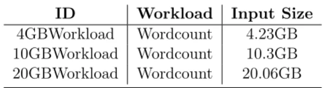
Table 6.6: Configurations of the three larger workloads

4GBWorkload Wordcount 4.23GB

6.1.1 Pseudo-distributed Setup

For the pseudo-distributed setup, we chose a computer with 6th generation quadcore intel i7 processor and 16GB memory. Pseduo-distributed mode basically hosts a vir-tual machine that runs all the hadoop daemons on the same machine and is the first

(55)

place where hadoop developers perform their experiments. This mode is a bridge between the standalone mode and the fully distributed mode. Standalone mode is not tested for our framework as it does not support running HDFS and YARN, which are required to test our framework. Pseudo-distributed mode simulates a real cluster on a single machine and provides a veritable test enironment for our experiments. For the pseudo-distributed setup, we perform experiments by running each job sep-arately as well as running multiple jobs concurrently. Tables 6.1, 6.2 and 6.3 show the configurations of the jobs in the experiments for each of the two sets of aforemen-tioned workloads. Both tables list all the jobs that were run separately and together. We configured the system to run at most 4 map tasks and 4 reduce tasks in parallel for each job by setting the configuration parametersmapreduce.job.running.map.limit

and mapreduce.job.running.reduce.limit in hdfs-site.xml. For the pseudo-distributed

mode we performed experiments with two different replication factors for the HDFS blocks, which are 1 and 3 (default replication in Hadoop). Additionally, we have con-ducted experiments while varying the hdfs block size to be 64MB, 128MB or 256MB.

6.1.2 Fully Distributed Setup

For the experiments in fully distributed mode, we utilized a cluster containing 5 nodes. Each of the nodes were implemented as virtual machines using VirtualBox [43], a powerful virtualization platform for x86 and intel/AMD64 architectures which is freely available as an Open Source Software to the scientific community under the GNU General Public License (GPL) version 2. All the virtual machines (VMs) are connected via 100Mbps ethernet links enabled by the bridged adapter using PCnet-Fast III (Am79C973) network driver. Table 6.3 shows the configuration of the nodes in this set up. Unlike the pseudo-distributed mode, we have not set any limit on the

(56)

3, which is the default hdfs replication. To evaluate the performance improvement in heteregenous or shared environments, we configured one of the nodes to be completely dedicated to be the master and it would not run any computation. Similar to the pseudo-distributed mode, we have conducted experiments while varying the hdfs block sizes between 64MB, 128MB and 256MB.

Table 6.7: Configurations of nodes in the cluster

Node ID Memory (MB) Disk Space Number of Virtual Processors

1 4GB 25GB 2 2 2GB 25GB 1 3 2GB 25GB 1 4 2GB 25GB 1 5 2GB 25GB 1

6.2 Evaluation Results

In this section, we present our evaluation results obtained through conducting ex-periments on the workloads described in Chapter 6.1. We present the results of the experiments on pseudo-distributed setup and fully distributed setup separately and discuss the results corresponding to each setup both separately and together. The metrics chosen for comparison are the percentage of locality improvement for the tasks, task execution times, total job completion time, total tasks killed and perfor-mance improvement compared to the default hadoop ecosystem.

(57)

6.2.1 Pseudo-distributed Mode

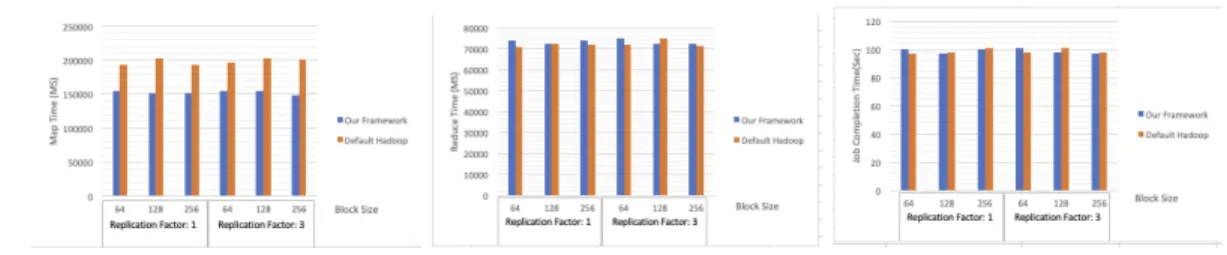
For the pseudo-distributed mode, we mainly looked at the execution time of map phase and reduce phase along with the total job completion time. Figures 6.1 to 6.8 show the results of the experiements that were obtained by running hadoop modified with our framework and the default hadoop over the workloads described in section 6.1. For each of the experiments, we present the total time spent in executing map phase, total time spent in executing reduce phase and the overall completion time of the jobs. Note that the graphs showing map times and reduce times is the total time spent by all maps and reduces (cumulative). Since multiple maps run in parallel, the value of map times and reduce times could be higher than the total job completion time, which is the total time taken for fininshing the job.

Figure 6.1: GutenbergSmall Workload

Figure 6.2: GutenbergLarge Workload

From the graphs, it can be observed that the execution times for map and reduce and the overall job completion times are better in most of the cases using our hadoop version compared to the default hadoop. This improvement was present with all three configurations of block sizes.

(58)

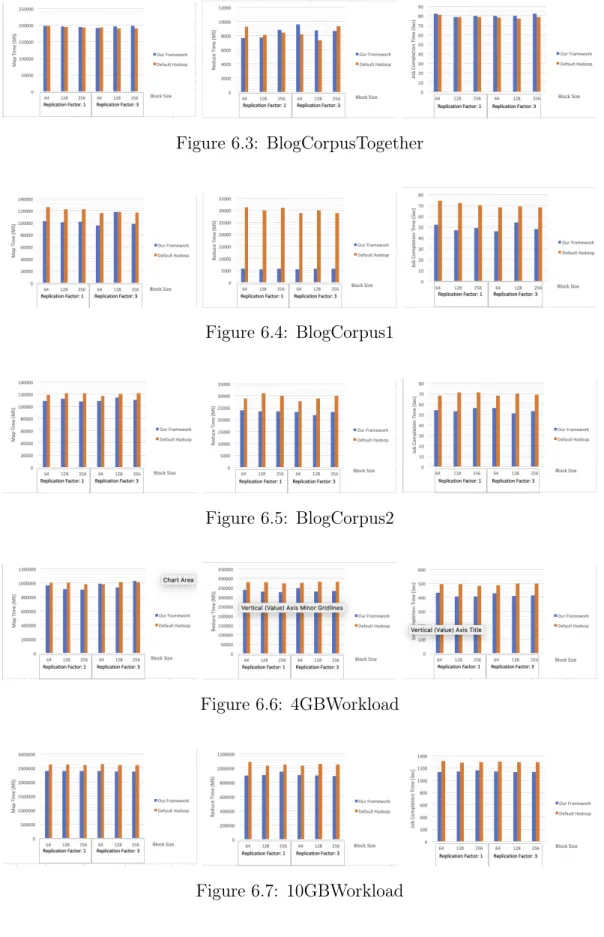
Figure 6.3: BlogCorpusTogether

Figure 6.4: BlogCorpus1

Figure 6.5: BlogCorpus2

Figure 6.6: 4GBWorkload