Robust Calibration of Macroscopic Traffic Simulation Models Using Stochastic Collocation

(1)

Transportation Research Procedia 9 ( 2015 ) 1 – 20

Peer-review under responsibility of the Scientific Committee of ISTTT21 doi: 10.1016/j.trpro.2015.07.001

ScienceDirect

21st International Symposium on Transportation and Traffic Theory, ISTTT21 2015, 5-7 August

2015, Kobe, Japan

Robust Calibration of Macroscopic Traffic Simulation Models using

Stochastic Collocation

Sandeep Mudigonda

a*

_{, Kaan Ozbay}

b

a_{Post-doctoral Fellow, Ph.D., Department of Civil and Urban Engineering, New York University, Six Metrotech Center, 4th Floor, Brooklyn, NY,}

11201, USA

b_{Professor, Ph.D., Center for Urban Science + Progress (CUSP); Department of Civil & Urban Engineering, New York University (NYU); One}

MetroTech Center, 19th Floor, Brooklyn, NY 11201, USA

Abstract

The predictions of a well-calibrated traffic simulation model are much more valid if made for various conditions. Variation in traffic can arise due to many factors such as time of day, work zones, weather, etc. Calibration of traffic simulation models for traffic conditions requires larger datasets to capture the stochasticity in traffic conditions. In this study we use datasets spanning large time periods to incorporate variability in traffic flow, speed for various time periods. However, large data poses a challenge in terms of computational effort. With the increase in number of stochastic factors, the numerical methods suffer from the curse of dimensionality. In this study, we propose a novel methodology to address the computational complexity due to the need for the calibration of simulation models under highly stochastic traffic conditions. This methodology is based on sparse grid stochastic collocation, which, treats each stochastic factor as a different dimension and uses a limited number of points where simulation and calibration are performed. A computationally efficient interpolant is constructed to generate the full distribution of the simulated flow output. We use real-world examples to calibrate for different times of day and conditions and show that this methodology is much more efficient that the traditional Monte Carlo-type sampling. We validate the model using a hold out dataset and also show the drawback of using limited data for the calibration of a macroscopic simulation model. We also discuss the drawbacks of using a single calibrated model for all the data.

Peer-review under responsibility of the Scientific Committee of ISTTT21

Keywords: calibration; stochastic collocation; macroscopic traffic flow

*_{Corresponding author. Tel.: +1-718-260-3960; fax: +1-(646)-997-0560.}

E-mail address: [email protected]

(2)

1.Introduction

Traffic simulation models are mathematical abstractions of the transportation system in which output is derived from a particular set of mathematical equations and relationships given a specific input data. The input data consists of two main groups of data sets: physical input data Is (e.g., volume counts, capacity and physical features of roadway sections) and driver specific parameters Cs (i.e., adjustable components of driver behavior such as free flow speed, reaction time, mean headway, etc.). Output from a simulation model can be expressed as shown in equation (1). The process of calibration entails adjusting the calibration parameters (Cs) so that the error between the output from simulation and field observations is minimized.

: ( , ) | ,

( , ) functional specification of the internal models in a simulation system

simulation output data given the input data and calibrated parameters, margin of error b obs s s sim s s s s sim O f I C O I C f I C O

H

o

etween simulation output and observed field data, and, observed field data.

obs O

(1)

Traditionally traffic simulation models are used to study scenarios for a certain time period of a so called “typical day”. However, as shown in Ozbay et al. (2014), the determination of a typical day is not a trivial task or a typical day may not even exist in reality. In fact, the typical day scenario might not also be the best scenario to test the effectiveness of operational strategies. Moreover, there is an increasing trend for using well-calibrated simulation models as predictive tools for real-time traffic control (Vasudevan and Wunderlich (2013), Yelchuru et al. (2013), USDOT ICM, Olyai (2011), Dion et al. (2009)). Clearly, these simulation models have to work under a combination of conditions that will considerably deviate from the typical day scenario.

Thus, calibration parameters estimated using limited sample data are not always representative of all possible conditions of the simulated system and might thus result in inaccurate predictions. In other words, models that are not adequately calibrated cannot accurately capture time-varying conditions of traffic. Traditional sources of traffic data used in the calibration of traffic models are either limited by the availability of the data that only cover typical conditions or may not be reliable enough. However, with the advent of new information technologies, unprecedented wealth of calibration data is on the fingertips of users by means of connected vehicles, smart phones, GPS-equipped devices, RFID readers among others. This, in turn, has led to massive amount of passively collected location and event data for various time periods. These data provide an opportunity to validate and calibrate traffic simulation models for a variety of spatio-temporal conditions.

Variability can be incorporated within inputs (demands) Is and calibrationparameter set (supply) Cs during different periods of the day, weather conditions, driver population composition, highway geometry, etc. There were previous studies that captured traffic variability (Li et al. (2009), Ngoduy (2011), Zhong and Sumalee (2008), Jabbari, Liu (2012), Lee and Ozbay (2009)) to name a few. However, the increase in the number of factors affecting stochasticity increases the dimensionality of the calibration process. This in turn results in increased computational effort required in calibrating traffic simulation models for different conditions such as variability within weekday/weekend, and seasonal variability, and special situations including adverse weather, work zones, etc.

In this study, we propose a novel calibration methodology to address the computational complexity due to the need for the calibration of simulation models under highly stochastic traffic conditions. We show the utility of larger datasets to capture variability in traffic flow and speed for various time periods.

2.Literature Review and Motivation

Typically, accurate modeling traffic flow requires three types of data: model inputs, model parameters and observed outputs. Model inputs involve the demand-side data for which the traffic simulation is performed. Model parameters involve different types of supply-side parameters used in the traffic simulation depending on the level of complexity in modeling. The output data observed in real-world is required to compare model outputs and evaluate the accuracy of the models.

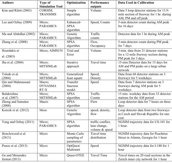
There are myriad of studies that deal with the calibration of traffic simulation models using various types of input and output data. Due to space constraint, we show a selected sample of them in Table 1.

(3)

Table 1 Summary of Literature on the Calibration of Traffic Simulation Models

Authors Type of

Simulation Tool

Optimization Performance outputs

Data Used in Calibration Kim and Rilett (2003) CORSIM,

TRANSIMS

Simple algorithm

Volume Data 5 loop detector stations for 13.9-mile section of freeway for 1 hr. during AM, PM and off peak

Lee and Ozbay (2009) Micro; PARAMICS

Enhanced- SPSA algorithm

Speed, Counts 5-min detector count during AM peak for 16 days

Ma and Abdulhai (2002) Micro;

PARAMICS Genetic Algorithm Traffic counts Detector data for 1 hr during AM peak Zhang et al. (2008) Micro;

PARAMICS

SPSA algorithm

Flow, Occupancy

5-min detector count during PM peak for 7 days

Hourdakis et al. (2003)

Micro; AIMSUN Trial and Error

Volume 5-min. data from 21 detector stations for a 12-mile freeway section during PM peak for 3 days

Jha et al. (2004) Micro; MITSIMLab

Iterative approach

Travel time 15-min Detector data for 15 days for AM and PM peaks on a large urban network Toledo et al. (2004) Micro; MITSIMLab Generalized least square Speed, Density

Data from 68 detector stations on 3 freeways for 5 weekdays

Qin and Mahmassani (2004) Macro; DYNASMA RT-X Transfer function model

Speed Data from 7 detector stations on 3 freeways during AM peak for 5 weekdays Balakrishna et al. (2007) Micro; MITSIMLab SPSA algorithm Traffic Counts

15 min. weekday data from 33 detector stations for the AM period

Zhong and Sumalee (2008)

Macro SPSA algorithm

Flow Loop detector data for 7 hours on three days

Korcek et al. (2012) Meso Genetic Algorithm

speed, density, flow

Loop detector data from two freeways in Czech and Slovak Republic for one year

Yang and Ozbay (2011) Micro; PARAMICS

SPSA algorithm

traffic conflict, lane change, volume & speed

NGSIM trajectory data for US-101 for 1 hour.

Henclewood et al. (2013)

Micro Monte Carlo

sampling of parameters

Travel time distribution

NGSIM trajectory data for Peachtree Street in Atlanta, Georgia for 1 hour

Punzo et al. (2013) Micro OptQuest Multistart

Speed NGSIM trajectory data for I-180 for 1 hour

Ge and Menendez format (2013)

Micro Quasi-OTEE Travel Time Travel times on 20 road sections in the Zurich inner city network for 1 hour

The effect of data and parameter uncertainty in traffic simulation models has received considerable attention recently (Henclewood et al. (2013), Punzo et al. (2013), Ge and Menendez (2013)). Studies from other fields indicate that bias and variance in simulation output results are due to the bias and variance in the input models used, after simulation error is eliminated; the input models consist of simulation model inputs and parameters.

(4)

if George E. Haver’s statistic, GEH < 4 ( 2 , , 1 , , 1 1 ( ) 1 ( ) 2 T sim i obs i i T sim i obs i i O O T GEH O O T

¦

) for link volumes for 85% of the links

and average travel times are within 15% of observed values, then it is considered as a satisfactorily calibrated model (Dowling et al. (2004)). In order to achieve this level of calibration for various conditions (peak, off-peak, weekends, normal and inclement weather, under accident, and other events), detailed level of data is required.

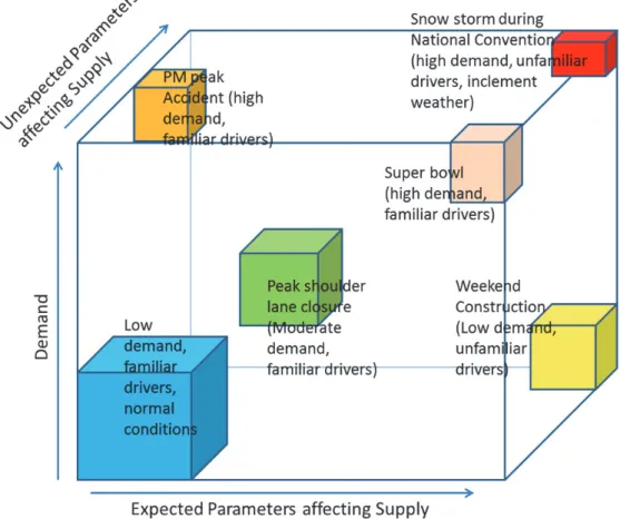
Table 1 also shows the data used in each study for the calibrating process. It can be seen that in most studies data used for calibration is a small set of traffic conditions and/or time periods no more than a few days. Thus, the data captures only a few specific conditions, or is a dilute sample of different conditions. As depicted in Figure 1, using only smaller samples of data will not accurately capture variation in traffic data. Hence, it is expected that the model predictions will only be accurate for those specific conditions. Using these models for conditions other than the ones for which calibration data was available for would not yield accurate results.

Thus the traditional approach of calibrating for a typical day is not sufficient, especially, if the calibrated models are used as predictive models. In addition, Ozbay et al. (2014) showed that the existence of a “typical” day in traffic demand is not always likely. Hence, to obtain accurate predictions from a traffic simulation model, it is important to consider not only the demand- and supply-side variation from various clusters, but also the demand- and supply-side variations within each cluster.

(5)

2.1.Computational Complexity

Calibration of traffic simulation model entails repeated execution of the simulation by varying the supply-side parameters and demand-side inputs until the error in outputs is minimized according to certain criteria. With so many variables, it is necessary to have a systematic approach to determine which parameters are important and how many replications of the simulation are necessary. Also, it is important to find the effect of each of these parameters and/or any interaction between them, before running the simulations for the combinations of parameters. This is the process generally called the experimental design.

Suppose there are k parameters. One approach is to vary the level of one parameter and keep all other k -1 parameters fixed. However, this is not an efficient approach and it may not be effective in determining the interaction between the parameters. A more efficient method is to have two levels for each parameter and execute the simulation at each of the 2k_{number of combinations. This approach is called the}₂k_{factorial design. (Law and} Kelton (2003))

When designing for an experiment with 2 distinct values in the discretized form for the n stochastic inputs (demands) would involve a full-factorial design i.e. with 2n_{replications. Additionally, the model has, say, 2} parameters with l and m distinct values (traffic conditions), the number of replications would be m*l*2n_.

Furthermore, due to the stochastic nature of the inputs, just two levels of inputs may not always be enough. For statistically significant results, the number of replications needed to be at a level of precision Ȗ, estimated standard

deviation S, and t-statistic for M-1 degrees of freedom, significance level Į is given by

2 1,1 /2

*

M

t

_D

S

J

§

· ¨

¸

©

¹

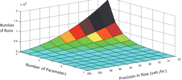
(Law and Kelton (2003)). Most studies capturing stochasticity in computational traffic models use a Monte Carlo (MC)-type independent sampling of M simulation runs for various traffic conditions. However, the convergence rate for MC-type method or Latin hypercube sampling is slow, O(1/¥M) (Loh (1996)).

To illustrate the computational burden for MC-type sampling, suppose we intend to simulate a freeway section with an on- and off-ramp. There are three independent demand inputs, namely, mainline, on- and off-ramp demands. Let’s suppose there are two stochastic parameters sampled at 10 points each and let’s also suppose that the standard deviation of demand is 140. To achieve a precision of 100 veh/hr in flow at 90% level of significance, the number of replications for variance reduction is 8. Thus the total number of runs required is 10*10*83_{= 51,200. If each run} takes 5 s (for instance), then the computational time taken = 71 hrs. If we want to increase our precision to further reduce the variance, the number of runs and computational time increases exponentially, as illustrated in Figure 2.

Figure 2 Illustration of number of runs required for statistically significant results using MC-type sampling with number of parameters and precision of estimation

(6)

In cases where large sources of data spanning different conditions are available, to capture the stochasticity in traffic conditions, there is also an increase in number of factors of stochasticity. This in turn increases the dimensionality of the calibration process. Thus depending on the size of the network and number of stochastic dimensions, MC-type sampling approaches can become prohibitive in terms of computational effort. It may not be possible at all to simulate the output for each and every possible realization of parameter and input. Also, all possible points in the stochastic space of simulation output may not have the corresponding observed data. Thus it is important to obtain an effective sampling and interpolation methodology for predicting output accurately but with lower computational effort.

3.Methodology

The proposed calibration methodology involves and initial exploration of output data to categorize into various distinguishable groups or clusters. Then for each output cluster, the input and parameter distributions are subsequently discretized using the stochastic collocation approach and calibration is performed. Each step is explained in detailed below.

3.1.Data Exploration

Based on the discussions above, making accurate predictions using traffic simulation models require calibration data in great detail. Various demand, speed, flow and event data can be obtained from different data sources.

In order to capture changing traffic conditions, we use traffic sensor data. As mentioned in the earlier section, traditionally, an arbitrarily chosen day or a collection of few days from the sample has been used for calibration. However, as depicted in Figure 1, this may not be representative of the speed and flow variations of the section. In order to capture the true variations in speed and flow of the section, we should use the output from a much larger sample of the population. The variation in the output of the freeway section could be due to reasons such as time of day, weather, construction, incidents, geometry, or even due to differences in acceleration or deceleration of drivers. One or more of these conditions could result in the variation of the section output. It is prudent to calibrate the simulation model separately for each of such condition resulting in the observed output. In other words, based on our analysis of the observed data, we claim that one set of global parameters that provide the best results for all conditions might not be a feasible approach for this problem dealing with very diverse conditions especially for very different conditions that have significant representation in the observed data.

In order to classify the section outputs, we use well-known clustering techniques. Clustering techniques are usually applied in initial investigation of data. However, it is an effective method to separate data into groups by minimizing variance within the group and maximizing variance between groups. The section output that falls into a group can be considered to be subjected to similar conditions. Hence, the simulation inputs and parameters that can be used to generate these conditions are considered as similar.

Simulation inputs form the demand-side of the freeway section and simulation parameters form the supply-side of the freeway section. The variation in the observed output of a freeway section could be a result of variation in the supply- or demand-side of the freeway section. In general, changes in free flow speed is a result of changing pavement condition, geometry or surrounding conditions, and thus is a property of the supply-side of the freeway section. In this paper, we use free flow speed to distinguish the variation in supply-side conditions. Furthermore, we use the speed output to further separate traffic conditions for the calibration of the freeway section for various conditions. Subsequently, we consider the variation in demand to capture the variation in output within each traffic condition.

The separation into different conditions using system output signifies the influence of distinguishable external conditions, such as weather, workzones, special events, etc. Thus each of the clusters corresponds to a different type of condition.

Speed output from the traffic sensors is used to categorize various traffic conditions. The demand data is obtained for various clusters of traffic conditions so as to use a distribution of demand for each condition. The simulation is performed using the clustered demand data distribution and simulation output of flow and density is compared to the observed distribution from sensor data.

(7)

3.2.Stochastic Collocation

As mentioned earlier, there is a need to combat the issue of high number of replications and dimensionality when using MC-type methods in capturing stochasticity using traffic simulation models. Stochastic spectral methods provide an efficient alternative to MC-type methods. In these methods, stochasticity is treated as another dimension and the infinite dimensional stochastic solution space ȍ is discretized and approximated by N-dimensional stochastic space ī. One such stochastic spectral method is the stochastic collocation (SC), where the approximation is performed by using deterministic solutions at a set of prescribed nodes (collocation points) and an interpolation function.

The notation to be used in this subsection and the rest of the paper is as follows:

1

( , ) : roadway density

D: deterministic space-time ( - ) domain : stochastic space

: finite dimensional approximation of

( ) : joint probability density function of random vector { , N i i x t D x t p [ [ u : : * : {

* ȡ ȟ ȟ ȟ

^ `

2 1 ,..., }, with support on ˆ interpolant using Lagrangian interpolation

: approximated with points ( ) = interpolating basis polynomials ( , ) = the deterministic solution for de

n i Q j _j k j j I Q x t [ [ U : * * ) ȡ ȥ ȥ ȥ nsity at ˆ

( ) expected value of density

j (

ȥ ȡ

For a set of Q points in the stochastic space where the simulation output is generated,

^ `

1

Q

j j

*

ȥ

, the

polynomial interpolation and estimation of expected value of density can be shown using equation (2), (Xiu and Hesthaven (2005)) 1 1 ( , ) ( , , ) ( ) ˆ( , , ) ( , , ) ( ), ˆ ( ( , , )) ( , , ) ( ) ( ) Q j j k j j Q j j k j x t x t p d I x t x t x D x t x t p d

U

\

\ \

* * | ) ( )

³

¦

³

ȡ ȡ ȟ ȟ ȟ ȡ ȥ ȥ ȥ ȡ ȥ ȥ (2)

The choice of weights, i.e., the basis functions

)

k , in SC depends on the interpolation technique. The approximation of expected value of density using MC-type sampling can be expressed as,

1 ˆ ( ( , , )) ( , , ) ( ) Q MC j j j j x t

U

x t p ( ȡ ȥ

_¦

ȥ ȥ ₍₃₎

From equations (2) and (3) we can see that the representation using SC interpolation and an MC-type sampling are similar. However, it is important to note that, unlike MC-type sampling methods, the weights assigned to each deterministic output is different in stochastic collocation methods. Thus SC interpolation can be applied in most cases where MC-type sampling is, potentially, applied such as mesoscopic or microscopic traffic simulation models. We do recognize that the applicability of the proposed methodology to other, more complex models is to be further studies. However, we suppose that the generic nature of the framework would provide that flexibility.

(8)

points (Ganapathysubramaniam and Zabaras (2007), Klimke (2006)) at higher dimensions of stochasticity. Smolyak algorithm, developed originally for multi-dimensional integration, entails evaluating deterministic solutions at the nodes of sparse sampling grids and building the interpolation function. One dimensional interpolant, with the Smolyak algorithm, is similar to equation (2) and given by equation (4),

1

( ) ( ) ,

( ) deterministic soluation at , interpolation basis polynomial, no. of nodes at level of interpolation .

one-dimensional interpolant at level

i m i j j j j j j i i U f f L f L m i U i

¦

ȥ ȥ ȥ (4)

However, when extending to multiple dimensions, since each stochastic dimension is independent, the interpolant in N-dimensions involves tensor products of one dimensional interpolants

U

i1

,...,

U

iN _{. Sparse} interpolant in N-dimensions and q-N interpolation order is given by equation (5),

1 1 , 1 , 1, 1 ( 1) ( ... ), where,

: Sparse interpolant in N-dimensions and q-N interpolation order q-N: interpolation order

0,

,..., : one dimensional interpolants

N N q i i q N q N q q N N N i i N A U U q A A U U d d § · _¨ _¸ © ¹

¦

i i i i 1 1,..., with 1 ...

... N : Tensor product of the one-dimensional interpolants

N N i i i i i i U U i (5)

The sparse grid at the points of which the deterministic solution is evaluated is defined as,

1 ( ) ( ) , , ( ) 1 1 ( ... )

: Sparse grid in N-dimensions and q-N interpolation order : grid points in dimension ,

,..., with ... , N j i i q N q q N i N N H H j i i i i \ \ \ u u i i i

*

(6)

Determining the grid

H

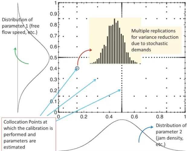
_{q N}_, is an important part of the Smolyak algorithm for interpolation. The distribution of points on the grid is usually performed using piecewise linear basis functions (Clemshaw-Curtis grid) or polynomial basis functions (Chebyshev-Gauss-Lobatto grid) (Klimke (2006)). An illustration of the discretization of the stochastic space using a Clemshaw-Curtis grid in two dimensions is shown in Figure 3. The stochastic probability space is projected onto the [0,1] X [0,1] probability space for the two stochastic parameters that follow Gaussian distribution. We perform the sampling, where the simulation runs are performed, at each of the sparse grid points. At each collocation point we use the probability value to obtain the value of the parameter using the inverse distribution. Thus at each point a deterministic form of the simulation is performed. The stochastic output distribution is constructed using the sparse grid interpolation of deterministic outputs and probability values obtained at each collocation point. For the sake of brevity we only show the sampling sparse grid for two stochastic parameters. This grid can be extended to multiple dimensions for other stochastic parameters and demand.

(9)

Figure 3 Example of approximation of stochastic space by collocation points

The advantage of this recursive/nested structure is that to increase the order of interpolation (accuracy) we can use all the deterministic solutions from the previous steps: Aq-1,N, by adding a few more deterministic solutions. When new data is available, additional deterministic solutions can be evaluated and accuracy of interpolant will be improved.

Convergence rate of the interpolant is of the order, O(Q-2_|logQ|3(N-1)_{) (for piecewise linear basis), O(Q} -k_|logQ|(k+2)(N-1)_{) (for}_k_{-polynomial basis). This rate can be controlled by the polynomial order k} (Ganapathysubramaniam and Zabaras (2007), Klimke (2006)). Thus, we show using numerical examples that convergence of this interpolant is better than the more commonly used Monte Carlo method.

3.3.Parameter Optimization

The stochastic collocation points in the grid (illustrated in the previous subsection) are used to discretize the stochastic dimension of stochastic inputs as well as stochastic parameters. The process involved in the estimation of calibrated parameters is described below.

From each realization of the parameter set, using the demand distribution as an input, the simulation output distribution (e.g., flow or density distribution) is generated. This distribution is compared with the observed output distribution and using a test statistic (such as the test statistic from the Kolmogorov-Smirnov (KS) test), the error is estimated. This error is used as an objective function and is minimized as part of the multi-objective parameter optimization as shown in equation (7), using the simultaneous perturbation stochastic approximation (SPSA) algorithm (Spall (1992)). In our study the weights (w) used are the coefficients of variation of each output measure

(10)

from the observed data.

^

1 1 2 2

`

1

min ( , ( )) ( , ( )) where,

, - observed and simulated flows at location , - observed and simulated densities for location - parameter set for time period

t N Ob S k Ob S k i i t i i t i Ob S i i Ob S i i k t w U q q w U q q i i U U U U 4 4 4 4

¦

1 2 1 2 and iteration , - weights for the error measures

, - functions representing the error in flow and density

t k

w w U U

(7)

For the specification of error in the objective function in equation (7), in general, there are many possible measures. However, since in the calibration problem at hand involves comparing output distributions, non-parametric statistical measures are useful. There are many non-non-parametric statistical measures such as test statistics for Kolmogorov-Smirnov test, Anderson-Darling (AD) test, Cramer von Mises (CvM) test, etc. The K-S test is distribution free in the sense that the critical values do not depend on the specific distribution being tested. The A-D and CvM tests make use of the specific distribution in calculating critical values. (Stephens (1974)) Otherwise simulation has to be used to estimate the critical values for AD and CvM tests. This would add an additional layer of complication and computational time in the calibration process. We implement the proposed calibration framework in readily available high-level programming languages such as MATLAB, R, etc. Hence the ease of applicability of statistical tests should also be considered. In most packages, the AD and CvM tests require the distribution to be specified. Since, we do not know whether the observed speed or flow data to follow any particular distribution, pre-specification of distribution is difficult. For these reasons, we decided to use the K-S test statistic as the error estimate in the objective function in the optimization problem set in equation (7).

To summarize the proposed approach, first the output data exploration is performed to categorize output into statistically significant clusters. For each output cluster, a corresponding input/demand-side distribution and parameter/supply-side distribution are generated. These distributions are discretized using the stochastic collocation method. For each realization of the parameter set, the simulation is performed and the output distribution is generated using the demand-side distribution. This is compared to the observed distribution and error statistic is generated. If the error statistic is not satisfactory, the parameter set is updated using the SPSA algorithm (Spall (1992)) and the output distribution is re-generated. A flowchart of the sequence of steps in our proposed methodology is shown in Figure 4. The main advantages of using this proposed calibration methodology are the following:

1. Computationally more efficient than MC-type exhaustive sampling methods with effective interpolant to generate full distribution of simulation output.

2. Time consumed by the collocation approach can be further reduced by parallelizing the simulation under each condition,

(11)

Figure 4 The logic of the proposed calibration methodology

The proposed sparse grid SC methodology can be applied in most cases where MC-type sampling is, potentially, applied such as mesoscopic or microscopic traffic simulation models. We do recognize that the applicability of the proposed methodology to other, more complex models is to be further studied. However, we suppose that the generic nature of our framework would provide that flexibility.

4.Results

In order to illustrate the stochastic variation in traffic conditions, a three-lane section of the NJTPK turnpike at interchange 7 is chosen. Although, microscopic traffic simulation tools, such as PARAMICS or VISSIM, provide a detailed and relatively accurate platform for modelling, model building, calibration and execution can be very time consuming. When studying the effects of various stochasticities, we are going to focus on a first order macroscopic traffic simulation to model the traffic flow in the study section. The stochastic version of the first order macroscopic traffic flow model can be represented as shown in equation (8).

(12)

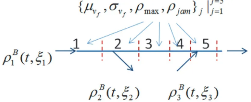
Figure 5 Schematic representation of the study section

max max ( , , ) ( , , ) 0 ( , , ) D: deterministic - domain : stochastic space

( , ( ), ( ), ( )) : fundamental relationship for cell for -th output cluster ( ) , ( ) , ( ) : sto t x j f jam i f j j jam j x t x t x t D x t f v j i v [ [ [ U [ U [ U [ [ U [ U [ w w u : : ȡ ȡv ȡ

chastic parameters for cell

( , ) B( , ) : stochastic input/demand in cell for -th output cluster

i j j i

j

x t t j i

U U [

(8)

We discretize the time and space for the model using the cell transmission model. In this study we adopt a Gaussian distribution for the free flow speed to characterize the stochastic fundamental diagram (Zhong and Sumalee (2008), Mihaylova and Boel (2006)). Thus the mean (ȝvf) and standard deviation (ıvf) of free flow speed form a part of the parameter set to be estimated along with critical density (ȡmax) and jam density (ȡjam). A schematic representation of the discretized simulated section, the stochastic input and model parameters is shown in Figure 5.

In this study, we use a hybrid of electronic toll collection (ETC) data for demand and traffic sensor data for speed and flow. The ETC data is collected at toll plazas on these freeways. (NJTA (2013)) The ETC dataset consists of the individual vehicle-by-vehicle entry and exit time data. It also consists of the information regarding the lane through which each vehicle was processed (both E-ZPass and Cash users), vehicle types, number of axles, etc.

In order to capture various traffic conditions, we use the traffic sensor data between for every 5 minutes between January 1, 2011 and August 31, 2011.This is, however, a very large dataset and can be considered as the population. We use a smaller sample of peak period during the months of April and May 2011 for calibration and use other parts of the larger dataset for validation. Even this sample of peak period during the months of April and May 2011 has a wide range of variation in speed and flow, as can be seen in Figure 6. Traditionally, an arbitrarily chosen day or days from this sample is used for calibration. However, as can be seen in Figure 6, this may not be representative of all the realizations of the speed and flow variations of the section. In order to capture the true variation in speed and flow, we would require using the output from the whole sample.

As mentioned in the methodology section, in order to classify the section outputs, we use k-means clustering. We follow the steps mentioned below in the clustering process:

1. Set up a desired number of clusters.

2. Group speed data from various days into clusters so as to minimize the sum of the differences between the day values and the mean for each cluster. (the procedure involved in k-means clustering)

3. As mentioned in the methodology section, the objective is to minimize the differences between data within clusters and maximize the difference between clusters. Hence, if the coefficient of variation (CoV) is more than 0.25 for any cluster, increase the number of clusters.

4.1.AM Peak Calibration Results

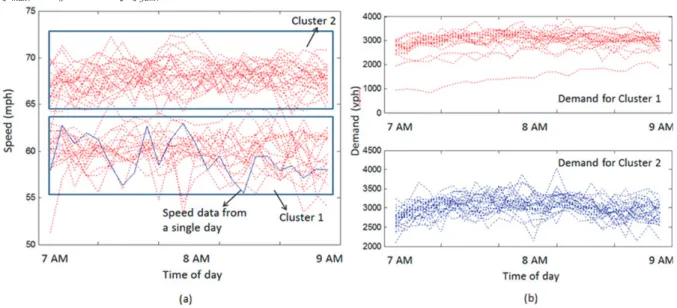
From Figure 6 (a), it can be seen that the speed output fell into two distinct groups with CoV less than 0.25 within each group. Hence, we consider two distinct traffic conditions in calibrating the macroscopic model for the

(13)

AM weekday peak. There are 24 and 19 days, respectively, falling under clusters 1 and 2. This shows that the possible reason for significant number of days with lower speed in cluster 1 is some activity that consistently takes place, such as long-term workzone or other maintenance activity. Such activity has been observed on the freeway section and thus characterizes the difference among the two conditions. We did not observe significant variation in speeds due to weather. It is likely that the demand-side could also have been impacted due to weather by neutralizing weather effects on the supply-side. Thus considering the distribution of demand during all the days encompasses the variation in demand due to weather conditions as well.

We calibrate the first order simulation model for each of these conditions separately and estimate the corresponding optimal parameters. Due to the variation in speed (shown in Figure 6 (a)), in this case study we propose to have a stochastic fundamental diagram that has a Gaussian stochastic free flow speed as mentioned earlier. Thus the parameter set involves mean (ȝvf) and standard deviation (ıvf) of free flow speed and critical density (ȡmax) and jam density (ȡjam).

Figure 6 (a) Illustration of speed data variation for AM weekday peak period during April and May 2011 (b) Distribution of demand for each condition (cluster) for the mainline section at interchange 7 of NJTPK during AM weekday peak

To capture the demand-side variation, we obtain the demand distribution from days falling into each cluster. The variation in demand at this section is captured using the ETC data for every 5 minutes between January 1, 2011 and August 31, 2011. The demand variation corresponding to each condition/cluster during the AM weekday peak period is shown in Figure 6 (b). Additionally, the on- and off-ramp demand distributions are also generated using the ETC data.

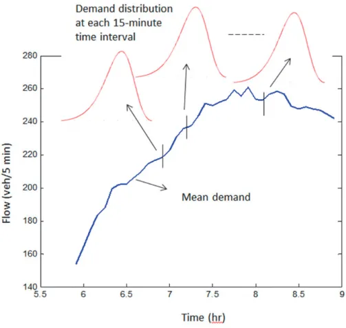
Thus for each cluster, the distribution of demand during each 15-minute time period is generated as illustrated in Figure 7. The calibration of the macroscopic simulation model is performed for AM peak (7-9AM). As mentioned in the methodology, with the demand distribution as an input, for each realization of the parameter set, the simulation output flow distribution is generated for cells 2 and 5 in Figure 5. This distribution is compared with the observed flow distribution at locations corresponding to cells 2 and 5, and using a test statistic the error is estimated. This error is used as the objective function for calibration and is minimized using the SPSA algorithm (Spall (1992)). The result of calibration is demonstrated using the comparison of simulated and observed flow.

(14)

Figure 7 Illustration of demand distribution at various sampled times

For this study, the Clemshaw-Curtis grid (two-dimensional version of which can be seen in Figure 3) is selected as the appropriate sparse grid to discretize the stochastic demand. The simulation is calibrated using the demand values at each of these grid points. The objective function for calibration is the test statistic used in K-S test at 90% significance, maximum separation between two distributions. As mentioned in equation (5), a sparse grid interpolation is performed for the output of the simulation and a Smolyak interpolant is constructed. Distribution of simulated flows is obtained by repeated evaluation of the Smolyak interpolation function. The simulated flow distribution is compared to the observed distribution from the sensor data.

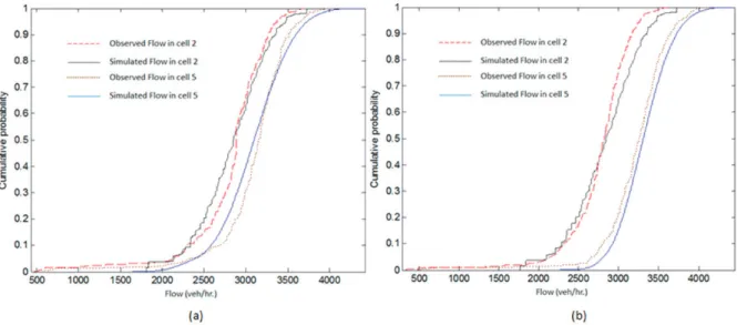
The comparison of observed and simulated flow distributions in cells 2 and 5 (Figure 5) from the calibrated model for AM weekday peak period for condition 1 is shown in Figure 8 (a). We noticed during the process of calibration that some cells have calibrated parameter sets different from the others. In other words, the stochasticity in simulation parameter set is not only temporal but also spatial. The calibrated parameters ([ȝvf, ıvfȡmax, ȡjam]) for AM weekday peak period for condition 1 are [53 2.11 85 150, 62 1.93 82 150] in appropriate units. The objective function (KS test statistic) after calibration is calculated as 0.09.

In order to compare the efficiency of the stochastic collocation approach, the distribution of simulated flow after model calibration is also generated using Monte Carlo sampling method. In order to achieve the flow distribution, the SC approach required 4034 evaluations for various stochastic demand combinations. However, using a MC-type sampling required 180,000 runs of the simulation model. The reason, as mentioned earlier, is due to the ability to construct efficient Smolyak interpolant that uses the simulation output from much fewer runs.

(15)

Figure 8 (a) Comparison of observed and simulated link flow distributions during AM peak period for condition 1 (b) Comparison of observed and simulated link flow distributions during AM weekday peak period for condition 2

Figure 9 Comparison of observed and simulated link flow distributions using limited data in calibrating AM peak period

The comparison of observed and simulated flow distributions in cells 2 and 5 (Figure 5) from the calibrated model for AM weekday peak period for condition 2 is shown in Figure 8 (b). Similar to condition 1, we noticed during the process of calibration that some cells have different calibrated parameter set from the others. The calibrated parameters ([ȝvf, ıvfȡmax, ȡjam]) for AM peak period for condition 2 are [50 1.64 83 150, 70 1.58 100 150] in appropriate units. The objective function after calibration is 0.08.

(16)

Carlo sampling method. In order to achieve the flow distribution, the SC approach required 3330 evaluations for various stochastic demand combinations. However, when using a MC-type simulation 180,000 samples were required to achieve the same level of significance.

Our main motivation behind using data from a variety of conditions is to capture the stochasticity in traffic conditions. To illustrate the drawback of using limited data, we compare the distribution of flow for AM period by using only one day’s speed and flow to calibrate the AM peak model. The simulated flow distributions (shown in Figure 9) from limited data model do not match, not only the AM peak flow data under cluster one but also the AM peak flow data under cluster two. In addition, the objective function after calibration is calculated to be 0.25. The objective function (test statistic of KS test) for calibration using the data from 43 days for conditions 1 and 2, respectively, are 0.09 and 0.08. This illustrates the drawback in using limited data for model calibration and the importance of considering stochasticity in traffic conditions when calibrating traffic simulation models.

4.2.PM Peak Calibration Results

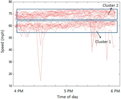
Similar to the AM weekday peak, clustering of speed data for PM (4-6PM) peak periods weekday is performed. Unlike the AM peak, the PM peak period speed data fell into six clusters. However, speed data from 33 out of 43 days (78% of data) fell into two clusters with CoV less than 0.25 for within each cluster. The CoV for the other clusters was in the range of 0.3-0.7. Also, the frequency of number of days within each cluster is not more than 4, indicating the speed data corresponding to these days as outliers possibly due to work zone conditions or incidents. Hence, we use the two major clusters as representative clusters. Figure 10 shows the speed variation among the two major clusters during PM weekday peak period. Hence, we consider two distinct conditions in calibrating the macroscopic model for the PM peak.

The comparison of observed and simulated flow distributions in cells 2 and 5 (Figure 5) from the calibrated model for PM weekday peak period for condition 1 is shown in Figure 11(a). Similar to AM peak, we noticed during the process of calibration that some cells have different calibrated parameter set from the others. In other words, the stochasticity in simulation parameter set is not only temporal but also spatial. The calibrated parameters ([ȝvf, ıvfȡmax, ȡjam]) for PM weekday peak period for condition 1 are [52 4.16 83 150, 62 2.85 90 150] in appropriate units. The objective function after calibration is found to be 0.08. In order to achieve the flow distribution, the SC approach required 1506 evaluations for various stochastic demand combinations. However, a MC-type sampling method to achieve the same accuracy required 9,000 runs of the simulation model.

(17)

Figure 11 (a) Comparison of observed and simulated link flow distributions during PM weekday peak period for condition 1 (b) Comparison of observed and simulated link flow distributions during PM weekday peak period for condition 2

The comparison of observed and simulated flow distributions in cells 2 and 5 (Figure 5) from the calibrated model for PM weekday peak period for condition 2 is shown in Figure 11(b). Similar to AM peak, we noticed during the process of calibration that some cells have different calibrated parameter set from the others. In other words, the stochasticity in simulation parameter set is not only temporal but also spatial. The calibrated parameters ([ȝvf, ıvfȡmax, ȡjam]) for PM weekday peak period for condition 2 are [48 2.26 80 150, 60 3.32 87 150] in appropriate units. The objective function after calibration is 0.05. In order to achieve the flow distribution, the SC approach required 1105 evaluations for various stochastic demand combinations. However, using a MC-type sampling required 9,000 runs of the simulation model.

In order to validate the estimated parameters using the proposed calibration methodology, we chose the month of July. Using the clusters generated for the speed observations for the weekday PM peak speed data April and May, we classify the speed data in July at interchange 7. This process resulted in 80% of the data falling into cluster two among the clusters generated for April and May. We generate the demand distributions for the mainline, on- and off-ramps using the ETC data for the days falling into the aforementioned cluster. Then we run the simulation separately for each clusters using the corresponding parameter set and demand distributions. The comparison of flow distributions is shown in Figure 12. The value of the objective function (KS test statistic) is found to be 0.084.

We test the effectiveness of calibrating a model with only one set of global parameters that best suits all conditions (called fixed parameter model). For this purpose we combine all the PM clusters and calibrate the model using the proposed approach. For the purpose of comparison and brevity, we call the model calibrated separately for different clusters as varying parameter model. We use the fixed parameter model to predict the flows for the PM peak period in July, performed similarly above using the varying parameter model. The comparison of flow distributions is shown in Figure 12. The value of the KS test statistic is found to be 0.29. This shows a statistically significant difference that the varying parameter model performs better than the fixed parameter model for the PM peak period in the month of July for the given freeway section. Though the data used to illustrate this idea spans a large time period and compares the distribution of output instead of single value of output, it is infeasible to test the statistical significance stated above for all possible times and freeway sections. Also as a generic marker for using a varying parameter model may be better to base the decision on the very diverse and different conditions that have significant representation in the observed data.

(18)

Figure 12 Validation of estimated parameters and comparison with fixed parameter model by comparison of flow distributions for major weekday PM peak days in July

5.Conclusions

The predictions of a well-calibrated traffic simulation model will be robust and reliable if variations in traffic are adequately taken into account when performing the calibration process. Variations in traffic conditions can arise due to many factors such as time of day, weather, existence of work zones, etc. Calibration of simulation models for a realistic range of traffic conditions requires larger than traditionally used datasets capturing the stochasticity in traffic conditions. Although larger datasets enables the modeller to more accurately capture the variation in data, this approach poses a challenge in terms of computational effort. With the increase in the number of stochastic factors, numerical methods employed for calibration of simulation models suffer from the curse of dimensionality. If, for example, traditional MC-type sampling is used, the computational effort required to calibrate traffic simulation models for various conditions could become intractable (as shown in Figure 2).

In this paper, we use electronic toll collection data and sensor data for a period between January 2011 and August, 2011. Also, we propose a novel calibration methodology to encapsulate stochasticity into macroscopic traffic simulation models and perform calibration with significantly reduced computational effort. We use stochastic collocation, a type of stochastic spectral method, to capture stochasticity in traffic. This method treats each stochastic factor as a separate dimension. Each dimension is discretized using a set of collocation points and an interpolant for the output is constructed using the simulation output at these points. In particular, we use the Smolyak sparse grid interpolation method due to the high number of stochastic dimensions.

The main advantages of using this methodology are the following:

1. Computationally more efficient than MC-type exhaustive sampling methods with effective interpolant, 2. Time consumed by the collocation approach can be further reduced by parallelizing the simulation under

each condition,

3. Nested form of the algorithm is useful in refining the interpolant as and when there is new data available. To demonstrate the usefulness of our methodology, we test it for an on-ramp-off-ramp section of NJTPK in the vicinity of interchange 7. The variation in supply- and demand-side parameters and inputs at this section is captured using the ETC and sensor data for every 5 minutes between January 1, 2011 and August 31, 2011. In order to

(19)

calibrate the model we use the AM peak period during April and May 2011. The system output is observed to be clustered into groups. The speed data is divided into clusters using k-means algorithm into two conditions during the AM and PM peak. Due to a significant number of days falling into each cluster, (24 and 19 for AM and 20 and 13 for PM), it is likely that the variation we observed is due to long-term workzone or maintenance activity. We did not observe significant variation in speeds due to weather. It is likely that the demand-side could have been impacted due to weather. Thus considering the distribution of demand during all the days encompasses the variation due to weather conditions as well.

The proposed methodology is applied to calibrate a macroscopic first order traffic simulation model for AM peak (7-9AM) and PM peak (4-6PM) for each condition/cluster. For calibrating the simulation model, we use the test statistic from the KS test for flow distributions on the link as the objective function. This objective function is minimized using the SPSA optimization algorithm (Spall (1992)). Due to the variation in speed (shown in Figure 6), in this case study we propose to have a stochastic fundamental diagram that has a Gaussian free flow speed distribution. Thus the mean (ȝvf) and standard deviation (ıvf) of free flow speed form a part of the parameter set to be estimated along with critical density (ȡmax) and jam density (ȡjam). We show that the comparison of simulated and observed flow distributions for the weekday AM and PM peak period for both conditions match well. We obtain completely different parameter sets for not only for each condition but also two different parameters for different sections of the freeway section. For AM, PM peak and conditions 1 and 2 the parameter sets are, respectively, as [53 2.11 85 150, 62 1.93 82 150], [50 1.64 83 150, 70 1.58 100 150], [52 4.16 83 150, 62 2.85 90 150], and [48 2.26 80 150, 60 3.32 87 150]. Additionally, we notice that the stochasticity in parameters is not only limited to time but also space. We show that the proposed methodology requires much fewer replications – about 88%-98% less – than MC-type sampling approach. Also we illustrate the advantage the proposed calibration approach by comparing simulated flow distributions generated from a model calibrated with a large set of demand and flow data and a model calibrated using limited days data. We validate the parameters estimated using the proposed methodology by running the model for the weekday PM peak days in July. The KS test statistic obtained for the flow distributions in July is found to be 0.084.

We test the effectiveness of calibrating a model with only one set of global parameters that best suits all conditions (called fixed parameter model) by comparing the flow distribution predicted by the two models with the observed flow distribution for PM peak period in the month of July. The value of the KS test statistic comparing predicted flow using fixed parameter model and observed flow is found to be 0.29, while the same for varying parameter model is 0.084 – almost a magnitude of order difference – for a larger and more complex network this difference is expected to be much larger. To make a statistically significant conclusion that the varying parameter model will always perform better on a global level, it has to be tested for all possible time periods and freeway sections. This is impractical to perform. However, as a generic marker for using a varying parameter model may be better to base the decision on the very diverse and different conditions that have significant representation in the observed data.

The proposed methodology could have a larger impact when calibrating microscopic simulation models. For example, PARAMICS microscopic simulation models described in Ozbay et al. (2013) such as the NJTPK and Jersey City models have about 2000 links with 100,000 vehicles traveling at any given time. Running one hour of such complex models takes about 30 minutes. Calibrating these models using an MC-type sampling method is infeasible for obvious computational reasons. Thus, the proposed methodology can be a very useful approach for calibrating microscopic traffic simulation models with varying complexity. This will be one of our major future directions.

Acknowledgements

The contents of this paper only reflect views of the authors who are responsible for the facts and accuracy of the models and results presented herein. The contents of the paper do not necessarily reflect the official views or policies of the any agencies.

References

Balakrishna, R., Antoniou, C., Ben-Akiva, M., Koutsopoulos, H. N., and Wen, Y., 2007. Calibration of microscopic traffic simulation models: methods and application. Transportation Research Record: Journal of Transportation Research Board, No. 1999: 198-207.

(20)

Boel, R., Mihaylova, L., 2006. A compositional stochastic model for real-time freeway traffic simulation. Transportation Research Part B 40 (4): 319–334.

Dion, F., Oh J. and Robinson, R. 2009. VII Testbed simulation framework for assessing probe vehicle snapshot data generation, Presented at the 88th Transportation Research Board Annual Meeting, Washington, D.C. (Pre-print CD-ROM).

Dowling, R, Skabardonis, A., and Alexiadis, V. 2008. Traffic analysis toolbox. Volume III: Guidelines for applying traffic microsimulation software. Publication FHWA-HOP-04-040. FHWA, U.S. Department of Transportation.

Ganapathysubramaniam, B., Zabaras, N., 2007. Sparse grid collocation schemes for stochastic natural convection problems. Journal of Computational Physics, 225: 652–685.

Ge, Q and Menendez, M., 2013. Sensitivity analysis for calibrating microscopic traffic model: A case study of the Zurich network in VISSIM, Presented at the 92nd Annual Transportation Research Board Annual Meeting, Washington, D.C. (Pre-print CD-ROM).

Henclewood, D., Suh, W., Rodgers, M.O., Hunter, M., 2013. Statistical calibration for data-driven microscopic simulation model, Presented at the 92nd Annual Transportation Research Board Annual Meeting, Washington, D.C. (Pre-print CD-ROM).

Hourdakis, J., Michalopoulos, P. G., and Kottommannil, J., 2003. A practical procedure for calibrating microscopic traffic simulation models. Transportation Research Record: Journal of Transportation Research Board, No. 1852:130-139.

Jabbari, S.E. and Liu, H.X., 2012. A stochastic model of traffic flow: Theoretical foundations. Transportation Research Part B 46, 156–174. Jha, M., Gopalan, G., Garms, A., Mahanti, B.P., Toledo, T., and Ben-Akiva, M.E., 2004. Development and calibration of a large-scale

microscopic traffic simulation model. Transportation Research Record: Journal of Transportation Research Board, No. 1876, 121-131. Kim, K. O. and Rilett, L. R., 2003. Simplex-based calibration of traffic micro-simulation models with intelligent transportation systems data.

Transportation Research Record: Journal of Transportation Research Board, No. 1855, 80-89.

Klimke, A., 2006, Uncertainty modeling using fuzzy arithmetic and sparse grids. Ph.D. thesis, Universitat Stuttgart, Shaker Verlag, Aachen. Korcek, P., Sekanina, L., Fucik, O., 2012. Evolutionary approach to calibration of cellular automaton based traffic simulation models, 15th

International IEEE Conference on Intelligent Transportation Systems Anchorage, Alaska, USA. Law, A.M. and Kelton, W.D. Simulation modeling and analysis (3rd ed.). McGraw-Hill, Boston, 2000

Lee J-B. and Ozbay, K., 2009. New calibration methodology for microscopic traffic simulation using enhanced simultaneous perturbation stochastic approximation approach. Transportation Research Record: Journal of the Transportation Research Board, No. 2124, Washington, D.C., 233–240.

Li, J., Chen, Q., Wang, H., Ni, D., 2009. Analysis of LWR model with fundamental diagram subject to uncertainties, Presented at the 88th Transportation Research Board Annual Meeting, Washington, DC (Pre-print CD-ROM).

Loh, W-L. 1996. On Latin hypercube sampling, The Annals of Statistics, 24(5), 2058-2080.

Ma, T., Abdulhai, B., 2002. Genetic algorithm-based optimization approach and generic tool for calibrating traffic microscopic simulation parameters. Transportation Research Record: Journal of Transportation Research Board, No. 1800: 6-15.

Menneni, S., Sun, C., Vortisch, P., 2008. Microsimulation calibration using speed-flow relationships: Making NGSIM data usable for studies on traffic flow theory. Transportation Research Records: Journal of Transportation Research Board, 2088. 1-9.

Ngoduy, D., 2011. Multiclass first order model using stochastic fundamental diagrams. Transportmetrica. 7(2). 111-125 NJTA. http://www.state.nj.us/turnpike/. Accessed December 25, 2013.

Olyai, K. 2011. Dallas area rapid transit. Integrated corridor management (ICM) initiative -Dallas demonstration Site. APTA 2011 Trans/Tech Conference, Miami, FL.

Ozbay, K., Mudigonda, S., Morgul, E., Yang, H., Bartin, B., 2014. Big Data and the calibration and validation of traffic simulation models, Presented at the 93rd Transportation Research Board Annual Meeting, Washington D.C. (Pre-print CD-ROM).

Punzo, V., Montanino, M., Ciuffo, B., 2013. Goodness of fit function in the frequency domain for robust calibration of microscopic traffic flow models, 92nd Transportation Research Board Annual Meeting, Washington, D.C. (Pre-print CD-ROM).

Qin, X., and Mahmassani, H. S., 2004. Adaptive calibration of dynamic speed-density relations for online network traffic estimation and prediction applications. Transportation Research Record: Journal of Transportation Research Board, No.1876, 82-89.

Spall, J. C., 1992. Multivariate stochastic approximation using a simultaneous perturbation gradient approximation. IEEE Transactions on Automatic Control. 37, 332-341.

Stephens, M. A., 1974. EDF statistics for goodness of fit and some comparisons. Journal of the American Statistical Association, 69, 730-737. Sumalee, A., Zhong, R.X., Pan, T.L., Szeto, W.Y. 2010. Stochastic cell transmission model (SCTM): A stochastic dynamic traffic model for

traffic state surveillance and assignment. Transportation Research Part B, 45. 507-533.

Toledo, T., Ben-Akiva, M. E., Darda, D., Jha, M., and Koutsopoulos, H. N., 2004. Calibration of microscopic traffic simulation models with aggregate data. Transportation Research Record: Journal of Transportation Research Board, No.1876: 10-19.

US DOT ICM Initiative. ICM Pioneer Sites – San Diego, California. http://www.its.dot.gov/icms/pioneer_sdiego.htm, <accessed August 28, 2014>

Vasudevan, M, and Wunderlich, K.. 2013. Analysis, modeling, and simulation (AMS) testbed preliminary evaluation plan for dynamic mobility applications (DMA) Program. Prepared by Noblis for USDOT, FHWA-JPO-13-097.

Wunderlich, K. 2002. Seattle 2020 case study, PRUEVIN methodology, Mitretek Systems.Report No. FHWA-OP-02-031.

Xiu, D., Hesthaven, J.S., 2005. High order collocation methods for the differential equation with random inputs. SIAM J. of Scientific Computing, 27. 1118–1139

Yang, H., and Ozbay, K., 2011. Calibration of micro-simulation models to account for safety and operation factors for traffic conflict risk analysis, 3rd International Conference on Road Safety and Simulation, Indianapolis, USA.

Yelchuru, B., Singuluri, S., and Rajiwade, S. 2013. ATDM Analysis, Modeling, and Simulation (AMS) Analysis Plan: Final Report (Draft). Prepared by Booz Allen Hamilton for the Federal Highway Administration, FHWA-JPO-13-022.

Zhang, M., Ma, J., Singh, S.P., Chu, L. 2008. Developing calibration tools for microscopic traffic simulation, Final report part III: Global calibration - O-D estimation, traffic signal enhancements and a case study. California PATH Research Report, UCB-ITS-PRR-2008-8. Zhong, R., Sumalee, A., 2008. Stochastic cell transmission model for traffic network with demand and supply uncertainties. Proceedings of the