CHARACTERISTICS OF A MARINE STRATOCUMULUS TO
CUMULUS CLOUD TRANSITION
A Thesis by
ALLISON LAUREN ZAPALAC
Submitted to the Office of Graduate and Professional Studies of Texas A&M University
in partial fulfillment of the requirements for the degree of MASTER OF SCIENCE
Chair of Committee, Anita D. Rapp
Committee Members, Courtney Schumacher Deborah J. Thomas Head of Department, Ping Yang
December 2014
Major Subject: Atmospheric Sciences
ABSTRACT
The studies in this thesis aim to improve the overall understanding of the characteristics of the marine stratocumulus to shallow cumulus transition over the southeast Pacific Ocean. This study uses observations from CloudSat and CALIPSO satellite instruments in NASA’s A-Train constellation to analyze environmental, microphysical and macrophysical cloud properties, precipitation, and cloud radiative effects along the climatological wind trajectories between January 2007 and December 2010. The interannual, intraseasonal, and diurnal variability of clouds across the transition over the study region is also examined.
Results show that as trade winds advect equatorward from the Peruvian coastline to warmer waters, thick, persistent, low-level stratocumulus clouds with high cloud fractions and strong shortwave cloud radiative effects in the southern portion of the study region gradually transition to shallow cumulus clouds with decreased cloud fractions and cloud radiative effects. The speed of this transition exhibits interannual, seasonal, and diurnal differences associated with changes in the large-scale environment. More frequent and intense precipitation along the trajectory corresponds to a more rapid reduction in cloud cover, implying that it may play a role in the transition through its reduction in cloud water and stabilizing effect on the boundary layer. Results also suggest that capturing the variability in the transition from stratocumulus to shallow cumulus clouds is important for improving representation of cloud feedback effects in current climate models.
ACKNOWLEDGEMENTS
I would like to express my sincere gratitude to my advisor, Dr. Anita Rapp, for her continued support, ideas, guidance, and patience throughout my work on this project. Words cannot express how much I appreciate the time and effort she has given me throughout my graduate studies, and for giving me the opportunity to continue my education. I would also like to thank my committee members Dr. Courtney Schumacher and Dr. Deborah Thomas for their guidance, support, and constructive feedback of my work throughout the course of this research.
Thanks also go to my friends and colleagues and the department faculty and staff for making my time at Texas A&M University a great experience. I also want to extend my gratitude to the National Science Foundation as this research would not have been possible without their support through the grant AGS-1128024.
Finally, I could not have done this without the patience, love and support of my husband Joshua, and to my amazing family for their encouragement, support, and unconditional love. I would not be where I am today without their unfailing love and support.
TABLE OF CONTENTS
Page ABSTRACT ... ii ACKNOWLEDGEMENTS ... iii TABLE OF CONTENTS ... iv LIST OF FIGURES ... vi LIST OF TABLES ... x 1. INTRODUCTION ... 11.1 Overview of clouds in the subtropical ocean ... 1
1.2 Overview of stratocumulus to cumulus transition ... 4
1.3 The southeast Pacific stratocumulus region ... 12
1.4 Main goals of thesis ... 16
2. METHODOLOGY ... 17 2.1 Data ... 17 2.2 Methods ... 24 3. RESULTS ... 34 3.1 Climatological representation ... 34 3.2 Interannual variability ... 45 3.3 Seasonal variability ... 55 3.4 Diurnal variability ... 65
4. SUMMARY AND DISCUSSION ... 72
4.1 Summary ... 72
4.2 Discussion ... 75
4.3 Limitations ... 79
4.4 Future work ... 80
LIST OF FIGURES
FIGURE Page
1 Illustration of processes important for stratocumulus formation and
development within the boundary layer.(Figure from Wood 2012) ... 3 2 Schematic showing structure of marine stratocumulus in (a) the shallow,
well-mixed boundary layer and (b) deeper, cumulus-coupled boundary layers. The gray arrows indicate the primary motions on the boundary layer scale, while smaller red arrows indicate the small scale entrainment mixing taking place at the inversion atop the layer. (Figure from Wood 2012) ... 6 3 GOES visible satellite images. (a) Open-cell mesoscale cellular convection
1445 UTC on October 18th and (b) closed cellular convection at 1445 UTC October 16th. The open-cellular structures are roughly 30 km across
(Comstock et al. 2005), whereas the cloudy portions of open cells are about 10 km (Wood and Hartmann 2004). (Figure from Comstock et al. 2005) ... 9 4 Illustration of key mechanisms that allow stratocumulus to form in the
southeast Pacific Ocean for the VOCALS field campaign. (Figure from
Wood et al. 2011) ... 13 5 Cloud fraction on the third day of the selected trajectories, and medians of
the forward (white line) and the backward (black line) climatological trajectories in the southeast Pacific and Atlantic Oceans. (Sandu et al.
2010) ... 31 6 Trajectory coordinate points (*) with the 2x 2 boxes around each of the
trajectory data points (*).The other points (+) are trajectory points calculated from the Appendix of Sandu et al. (2010) ... 31 7 Four-year mean representation of the environmental variables (a) SST in
°C(b) temperature profile (K), (c) the LTS (K), and (d) specific humidity (g kg-1), along the climatological wind trajectory in the southeast Pacific ... 35 8 Four-year mean representation of each cloud variable observed along the
climatological wind trajectory in the southeast Pacific. The panels are (a) cloud fraction (%), (b) cloud layer top and base heights (m), (c) optical depthduring the day (unitless), (d) effective radius during the day (microns), (e) non-precipitating cloud liquid water path (g m-2), and (f) total low cloud fraction (in %) ... 38
FIGURE Page 9 Four-year mean for (a) the rain frequency (% likelihood) and (b) the rain rate
(mm d-1) for all cloud observations .The red and blue lines in figure 8(a) represent the likelihood that rain is present at the surface over all
observations (blue) and the likelihood that rain is certain at the surface over all observations (red). The rain rate in Figure 8(b) is separated by the
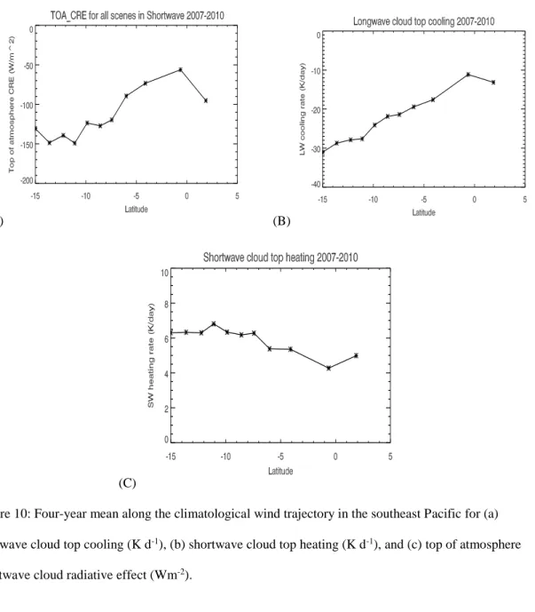
conditional (blue) rain rate and the unconditional (red) rain rate (mm d-1) ... 41 10 Four-year mean along the climatological wind trajectory in the southeast
Pacific for (a) longwave cloud top cooling (K d-1), (b) shortwave cloud top heating (K d-1), and (c) top of atmosphere shortwave cloud radiative effect (Wm-2)... 44 11 The sea surface temperature (°C) along the climatological wind trajectoryin
the southeast Pacific for each year relative to the 4-year mean(black dashed) .. 46 12 The temperature profile (K) along the climatological wind trajectory in the
southeast Pacific for 2007-2010. ... 47 13 The LTS (K) for each year relative to the 4-year mean climatology(black
dashed) ... 48 14 The specific humidity (g kg-1) along the climatological wind trajectory in the
southeast Pacific for 2007-2010 ... 49 15 The cloud fraction (%) along the climatological wind trajectory in the
southeast Pacific for (a) 2007, (b) 2008, (c) 2009, and (d) 2010 ... 51 16 Cloud layer top and base heights (m) along the climatological wind trajectory
in the southeast Pacific for 2007 ... 52 17 The LWP (g m-2) for each year relative to the 4-year mean (black dashed)
along the climatological wind trajectory in the southeast Pacific ... 53 18 The rain possible frequency (% likelihood) and conditional rain rate (mm
day-1) for cloud observations for each year relative to the 4-year
meanclimatology (black dashed) ... 54 19 The longwave cooling rate (K d -1) at the cloud top for each year relative to
FIGURE Page 20 The SST (°C) along the climatological wind trajectory in the southeast
Pacific for each season relative to the 4-year mean (black dashed) ... 57 21 The temperature profile (K) along the climatological wind trajectory in the
southeast Pacific for both (a) MAM and (b) SON ... 57 22 The LTS (K) along the climatological wind trajectory in the southeast Pacific
for each season relative to the 4-year mean (black dashed ... 58 23 The specific humidity profile (g kg-1) along the climatological wind
trajectory in the southeast Pacific for both (a) MAM and (b) SON ... 58 24 Cloud fraction (%) along the climatological wind trajectory in the southeast
Pacific for (a) DJF, (b) MAM, (c) JJA, and (d) SON ... 60 25 Cloud layer top and base height (m) along the climatological wind trajectory
in the southeast Pacific for (A) MAM and (B) SON ... 60 26 The LWP (g m-2) for each season relative to the 4-year mean climatology
(black dashed) ... 61 27 (a) The rain possible frequency (% likelihood) and (b) the conditional rain
rate (mm day-1) of cloud observations for each season relative to the 4-year mean climatology (black dashed) ... 62 28 The TOA shortwave cloud radiative effect (W m-2) for each season relative
to the 4-year mean climatology (black dashed) ... 63 29 The longwave cloud top cooling rate (K d-1) for each season compared to the
4-year mean climatology (black dashed) ... 64 30 The temperature profiles (K) for (A) day and (B) night ... 66 31 The cloud fraction (%) along the climatological wind trajectory in the
southeast Pacific for (A) daytime overpasses and (B) nighttime overpasses ... 67 32 The cloud layer top and base heights (m) for day (pink) and night (blue) ... 67 33 The LWP (g m-2) for day (pink) and night (blue). ... 68
FIGURE Page
34 The rain possible frequency (blue) and the rain certain frequency (red)for (A) day and (B) night ... 69 35 The conditional rain rates (mm d-1) for (A) day and (B) night ... 69 36 The longwave cloud top cooling (K d-1) for day (pink) and night (blue) ... 70
LIST OF TABLES
TABLE Page
1 Data products and variables used in research from 2007-2010 ... 20 2 List of coordinate points used in study and the total number of observations
1. INTRODUCTION
1.1 Overview of clouds in the subtropical ocean
Clouds cover nearly two thirds of Earth’s surface and have a significant impact on Earth’s climate through their influence on the radiation budget (Stephens et al. 1981; Ramanathan et al. 1989; Stubenrauch et al. 2010). High clouds both reflect incoming solar radiation and absorb outgoing thermal radiation emitted by the surface, generally leading to a warming effect of the atmosphere (Hartmann et al. 1992; Klein and Hartmann 1993; Kollias et al. 2004). Conversely, low clouds reduce the amount of incoming solar energy reaching the surface by reflecting sunlight back to space and absorb and emit nearly the same amount of longwave radiation as the surface (Hartmann et al. 1992), resulting in a cooling effect of the surface (Schneider 1972; Kollias et al. 2004). Over the subtropical oceans, low, optically thick stratocumulus clouds with their
limited vertical extent (cloud top heights rarely exceed 2 km), long-lasting, widespread coverage and their high albedo that reflects large amounts of incoming solar radiation, produce a strong cooling effect on earth’s climate.
Some of the largest uncertainties in the projections of future climate arise from the representation of clouds in climate models (Stephens 2005; Soden and Held 2006; Dufresne and Bony 2008), particularly in the representation of the physics of shallow clouds (Bony and Dufresne 2005; Webb et al. 2006). Because they cover vast areas of earth’s surface and are highly reflective to shortwave radiation, marine stratocumulus clouds have a significant impact on the climate system making them an important
component of radiation balance (Muhlbauer et al. 2014). They also contribute to the water cycle by transporting moisture from the surface to the free troposphere.
Understanding the physics of marine stratocumulus clouds is important for improving estimates of future climate prediction (Klein and Hartmann 1993; Stephens 2005; Teixeira et al. 2011). In particular, the parameterization of stratocumulus clouds in the marine boundary layer is a significant source of uncertainty in climate predictions (Bony and Dufresne 2005; Chung and Teixeira 2012). The complicated physical processes associated with the transition from marine stratocumulus to shallow cumulus clouds are particularly challenging to understand and predict, which is one of the reasons why the uncertainty is so large in global weather and climate models (Teixeira et al. 2011; Cheng and Xu 2013).
Marine stratocumulus clouds typically form on the eastern basins of the subtropical Atlantic and Pacific Oceans beneath a strong capping inversion that is associated with the descending branch of the Hadley cell where sinking motion occurs (Klein and Hartmann 1993, 1994). Extensive areas of stratocumulus clouds are
commonly observed as either solid or broken cloud decks in regions where warm, subsiding air is present over cooler sea surface temperatures (SSTs) (Klein and Hartmann 1993; Wood 2012). The strong subsidence helps to maintain the necessary temperature inversion, which keeps the boundary layer shallow and well mixed (Xu et al. 2004; Richter and Mechoso 2004, 2006; Wood 2012).
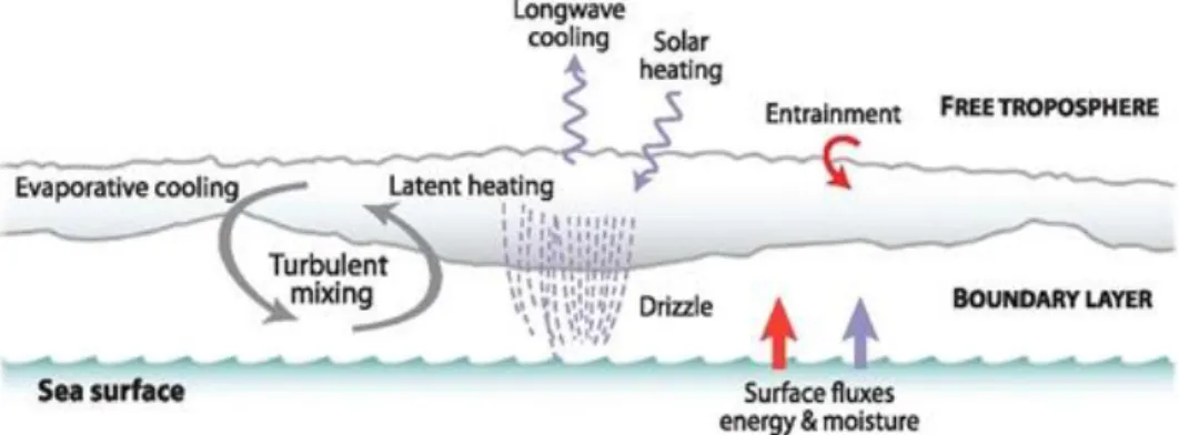
Figure 1 from Wood (2012) illustrates the general structure of stratocumulus clouds in the boundary layer and indicates the role of key processes such as radiative
heating and cooling, latent heating, surface fluxes, and entrainment within the cloud layer that impact the development and maintenance of stratocumulus clouds. Strong longwave radiative cooling at the cloud top drives the instability within the
stratocumulus cloud layer (Lilly 1968; Wood 2012). During the day, the absorption of solar radiation heats up the cloud layer and reduces the longwave radiative cooling and instability within the cloud layer, which leads to the gradual thinning and breakup of the stratocumulus cloud layer. During the overnight hours, the longwave radiative cooling increases, resulting in increased instability, stronger turbulence within the cloud, and more efficient cloud coupling with the surface moisture supply (Turton and Nicholls 1987; Rogers and Koracin 1992; Wood 2012). Therefore, the maximum stratocumulus cloud coverage occurs in the early morning hours before sunrise (Duynkerke et al. 2004; Wood 2012).
Figure 1: Illustration of processes important for stratocumulus formation and development within the boundary layer. (Figure from Wood 2012)
Latent heating released in the upward branches of the convective elements and evaporative cooling found in the downdrafts adds an additional source of turbulence to strengthen the convection (Moeng et al. 1992; Wood 2012). The turbulent mixing within the cloud layer controls the development of mesoscale organization and also frequently couples the cloud layer to the moisture source found at the surface (Nicholls 1984; Shao and Randall 1996). Both turbulent eddies and evaporative cooling drive entrainment at the top of the stratocumulus-topped boundary layer, which allows the marine boundary layer to deepen over time (Wood 2012). The surface latent heat flux, which is controlled by the relative humidity, temperature, and wind speed at the surface, provides the main source of moisture for the stratocumulus-topped boundary layer (Wood 2012).
1.2 Overview of stratocumulus to cumulus transition
As the trade winds advect air toward the equator over the warmer sea surface, the boundary layer warms and deepens (Krueger et al. 1995; Wyant et al. 1997; Wood 2012). Several studies have documented the changes in cloud structure of stratocumulus clouds as they advect equatorward (Albrecht et al. 1995, Bretherton and Wyant 1997). The Atlantic Stratocumulus Transition Experiment (ASTEX), conducted during June of 1992 in the northeast Atlantic, investigated the mechanisms and processes responsible for the uniform shallow stratocumulus to trade wind cumulus transition and showed that the processes involved in the decoupling of the surface and cloud layer were important for the stratocumulus to cumulus transition offshore (Albrecht et al. 1995). An increase
in convective activity over the warmer waters strengthened the turbulence within the boundary layer, leading to an enhancement of entrainment near the cloud tops
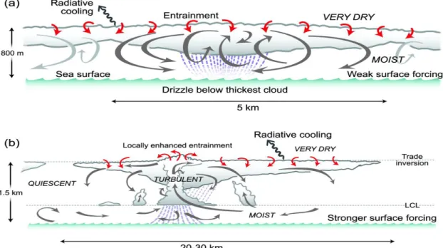
(Bretherton and Wyant 1997; Sandu et al. 2010). This enhanced entrainment helps to stabilize the stratocumulus cloud layer, therefore decoupling the cloud layer from the surface and inhibiting surface moisture from reaching the cloud layer. As this occurs, the environment near the surface is conditionally unstable and moisture is readily available, allowing shallow cumulus clouds to form underneath the stable cloud deck (Albrecht et al. 1995; Wang and Lenschow 1995; Sandu et al. 2010). As the developing cumulus clouds deepen, they recouple the stratocumulus cloud layer with the surface (Sandu et al. 2010). As the updrafts from the developing shallow cumulus clouds become vigorous enough to penetrate the inversion, they entrain warm dry air from above the boundary layer (Wang and Lenschow 1995; Bretherton and Wyant 1997). This weakens the temperature inversion and begins to thin and evaporate the stratocumulus deck until it breaks up into thin broken patches, leaving only shallow cumulus clouds (de Szoeke et al. 2006). By deepening the boundary layer and evaporating the stratocumulus cloud layer, shallow cumulus clouds help bring about the transition from stratocumulus to shallow cumulus clouds (Albrecht et al. 1995), causing cloudiness to decrease (de Szoeke et al. 2006). According to Sandu et al. (2010), this transition from stratocumulus to shallow cumulus clouds takes about 3 days. An overview of this transition is
illustrated in Figure 2 with the top panel representing a shallow, well mixed layer and the bottom panel representing a decoupled boundary layer.
Figure 2: Schematic showing structure of marine stratocumulus in (a) the shallow, well-mixed boundary layer and (b) deeper, cumulus-coupled boundary layers. The gray arrows indicate the primary motions on the boundary layer scale, while smaller red arrows indicate the small scale entrainment mixing taking place at the inversion atop the layer. Figure from Wood (2012).
In October - November 2008, the VAMOS Ocean-Cloud-Atmosphere-Land Study Regional Experiment (VOCALS-REx) studied boundary layer clouds on a transect along 20° S in the southeast Pacific Ocean (Bretherton et al. 2010). Bretherton et al. (2010) found that further offshore, the free tropospheric air was cooler and drier than along the coast, which weakened the inversion and further enhanced longwave cooling at the top of the cloud layer, thus allowing turbulence to strengthen within the cloud layer. This led to stronger entrainment and a deeper boundary layer further offshore (Bretherton et al. 2010). As the boundary layer deepened along the 20°S
transect, it created more variability in the liquid water path (LWP) and decoupled the vertical structure in the marine boundary layer, which allowed stratocumulus clouds further offshore to exhibit stronger organization, higher liquid water paths, and extensive drizzle (Bretherton et al. 2010).
Marine stratocumulus clouds frequently produce light precipitation, with drizzle as the most common form observed (Nicholls and Leighton 1986; Petty 1995; Austin et al. 1995; Wood 2005), as illustrated in Figure 1 (Wood 2012). A number of field
experiments have studied the formation and frequency of drizzle in stratocumulus clouds and its impact on the marine boundary layer (Austin et al. 1995; Stevens et al. 2003; Comstock et al. 2005). As previously mentioned, the longwave cooling at night helps to thicken the stratocumulus clouds, increasing the likelihood for precipitation to occur in the early morning hours. The formation of precipitation allows latent heat to be released and also removes water from the cloud layer, thus heating, stabilizing, and drying the cloud layer. Therefore, studies (Austin et al. 1995; Stevens et al. 2003; Comstock et al. 2005) have found that precipitation depletes both the cloud amount and cloud liquid water path and that the drizzling regime corresponds to increased variability of the properties that make up the cloud and boundary layer (Comstock et al. 2005). The evaporation of drizzle helps to cool and moisten the subcloud region, which contributes to stabilizing the boundary layer (Comstock et al. 2005). Simulations from Comstock et al. (2005) indicate that the evaporation of drizzle inhibits the heat and moisture flux beneath the nocturnal stratocumulus cloud layer. These conditions, like the strong drizzle events observed during the ASTEX campaign in the northeast Atlantic, are frequently
observed with patchy cloud conditions (Stevens et al. 1998) and suggest that open-celled cloud patterns correspond to heavy drizzle (Stevens et al. 2005).
Recent studies have focused on better understanding the role of precipitation in the transition from stratocumulus to shallow cumulus (Bretherton et al. 2004, 2010; vanZanten and Stevens 2005). There is evidence that precipitation may actually speed up the stratocumulus to shallow cumulus transition process (vanZanten and Stephens 2005). During Dynamics and Chemistry of Marine Stratocumulus II (DYCOMS-II), vanZanten and Stevens (2005) showed that localized patches of enhanced precipitation
corresponded with regions of open cellular convection (pockets of open cells) off the California coast. Pockets of open cells (POCs) are regions of open-cellular cloud
structures surrounded by or adjacent to regions of closed-cellular cloud fields (Stevens et al. 2005). Figure 3 from Comstock et al. (2005) illustrates the differences in the
boundary layer between an (a) open-cell and (b) closed cell mesoscale cellular convection in GOES visible satellite images. The closed cell structures often have surface convergence and updrafts where higher levels of moisture are present, which contribute to the replenishment of moisture into the cloud (Comstock et al. 2005). A POC sampled by airborne radar during the DYCOMS-II campaign (Stevens et al. 2003) showed that the POC region was comprised of mesoscale cells with enhanced
convection near the edges of the domain where locally higher cloud top heights and enhanced reflectivity that reached the surface (drizzle) were observed (Stevens et al. 2005). Stevens et al. (2005) also found that the interiors of these mesoscale cellular walls showed lower cloud top heights and even had regions of clearing, or low cloud fraction.
The study concluded that the observed high drizzle rates could likely stabilize the boundary layer, allowing shallow cumuli to develop and instigate a transition within the cloud structure (vanZanten and Stevens 2005; Stevens et al. 1998, 2005).
Figure 3: GOES visible satellite images. (a) Open-cell mesoscale cellular convection 1445 UTC on October 18th and (b) closed cellular convection at 1445 UTC October 16th. The open-cellular structures
are roughly 30 km across (Comstock et al. 2005), whereas the cloudy portions of open cells are about 10 km (Wood and Hartmann 2004). (Figure from Comstock et al. 2005)
Bretherton et al. (2004) observed drizzle when thick clouds were present in the overnight and early morning hours during a 2 week cruise in September of 2001 as part of East Pacific Investigation of Climate (EPIC). They concluded that the entrainment of dry air played a major role in influencing the thickness of stratocumulus clouds, but light drizzle could also reduce the amount of turbulence within the cloud. A POC was
observed during this field experiment as a boundary between open and closed cellular convection passed over one of the research vessels. The shipborne radar measured
frequent periods of higher reflectivity (a proxy for drizzle, e.g., Vali et al. 1998) that extended down to the surface (Stevens et al. 2005) when the region of open cells passed over.
The stratocumulus to shallow cumulus transition has been researched using several approaches, such as large-scale statistical studies (Klein and Hartmann 1993; Wood and Hartmann 2006), observational studies in a specific region (Bretherton et al. 2004, 2010; vanZanten and Stevens 2005), mixed layer modeling studies (Bretherton and Wyant 1997), and high resolution simulations (Krueger et al. 1995; Wyant et al. 1997), with each approach providing crucial information about the transition processes (Chung et al. 2012).
In a recent study, Sandu et al. (2010) performed an analysis of satellite observations and meteorological reanalysis along Lagrangian wind trajectories in stratocumulus to cumulus transitions. They composited thousands of individual Lagrangian trajectories over four subtropical regions within the Atlantic and Pacific Oceans where stratocumulus clouds are commonly observed and compared these trajectories to the climatological trajectories computed from the mean five-year wind field. After comparing the observations along the climatological and the individual trajectories, they concluded that the climatological trajectories are highly representative of the mean of the individual trajectories, partially due to the steady features found in the trade winds (Riehl et al. 1951, Sandu et al. 2010). Therefore, the climatological
trajectories can be used to represent the mean 3-day transition in clouds along the trajectory in the Southeast Pacific. Sandu et al. (2010) concluded that the transition,
which is characterized primarily by a decrease in cloud fraction, is mainly correlated with an increase in SSTs. Their study primarily focused on the changes in cloud fraction along the trajectories across the stratocumulus to shallow cumulus transition, rather than on the properties of the clouds or other factors, such as precipitation, that may be
important in this transition. Since the climatological trajectories were highly
representative of the 3-day transition from stratocumulus to cumulus, this analysis will use the climatological trajectories from Sandu et al. (2010) to study the cloud structure and radiative impacts across the transition in further detail.
This type of analysis has been previously applied by Teixeira et al. (2011) to evaluate weather and climate models along a cross section in the northeastern Pacific Ocean, from stratocumulus clouds situated off the coast of California across the trade winds where shallow convection dominates, to the ITCZ region where deep convection is prominent. Teixeira et al. (2011) showed that many of the weather and climate prediction models underestimated the amount of clouds in the stratocumulus regime, both in cloud cover and in liquid water path. They suggested that these underestimates occurred due to the timing of the transitions, as the transitions occurred too early in models compared to the observations (Teixeira et al. 2011; van der Dussen et al. 2013). They also found a large spread between models estimates of transitions in cloud cover, liquid water path, and shortwave radiation. While Teixeira et al. (2011) analyzed the cross-section of precipitation across the transition in the northeastern Pacific, the measurements they used are not sensitive enough to the light precipitation that is most prevalent across the transition from stratocumulus to shallow cumulus. This study will
apply a similar analysis technique along the Sandu et al. (2010) trajectories with satellite data over the southeast Pacific for a much longer period.
1.3 The southeast Pacific stratocumulus region
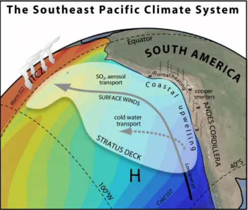
The interactions between the western portion of the South American continent and the Southeast Pacific (SEP) Ocean are important for both the regional and global climate system (Wood et al. 2011). Figure 4 from Wood et al. (2011) provides an
illustration of the mechanisms important for the stratocumulus cloud layer to form in this region. The Andes Cordillera (the longest mountain chain in the world), form a sharp barrier to zonal flow, resulting in strong winds (coastal jet) that flow parallel to the coasts of Chile and Peru (Garreaud and Muñoz 2004). There is also large-scale subsidence that occurs year-round over the southeastern Pacific Ocean, resulting in a quasi-permanent surface anticyclone that is centered roughly at 27°S, 90°W (Garreaud and Muñoz 2004). This subtropical high brings southern low-level winds along the coastline of Chile and Peru, which drives the strong oceanic upwelling along the coasts of Chile and Peru, bringing cold, deep, nutrient-rich waters up to the surface (Garreaud and Muñoz 2004, Wood et al. 2011). As a result, a tongue of cold surface water is found along the west coast of South America where the coastal sea-surface temperatures are colder along the Chilean and Peruvian coasts than at any comparable latitude elsewhere (Wood et al. 2011). Both the cold ocean surface and the warm, dry air aloft due to subsidence are ideal for the formation of marine stratocumulus clouds, and help to support the largest and most persistent subtropical stratocumulus deck in the world in
this region (Klein and Hartmann 1993, Bretherton et al. 2004, 2010). The subsidence that drives the development of stratocumulus is seasonally influenced by the downward branch of the Hadley cell, where a region of subsidence is located at 30°S (Liang and Evans 2011) and also influenced by location of the Walker circulation in the Pacific Ocean, which is an east-west circulation with rising air in the west Pacific and sinking air over the east Pacific Ocean (rather than the north-south circulation associated with the Hadley cell) (Liang and Evans 2011).
Figure 4: Illustration of key mechanisms that allow stratocumulus to form in the southeast Pacific Ocean for the VOCALS field campaign. (Figure from Wood et al. 2011)
The presence of this expansive and persistent cloud deck has a major impact on earth’s radiation budget, mainly due to high amount of reflected solar radiation, which acts to cool to surface below, resulting in a stronger inversion and tighter couplings between the upper ocean and the lower atmosphere. It is also likely that the transition from stratocumulus to shallow cumulus clouds in this region plays a significant role in cloud-climate feedbacks, which is one of the reasons why it is important to better understand the factors that control this transition (Teixeira et al. 2011; Chung et al. 2012).
Although a number of field experiments have improved the understanding of stratocumulus clouds in the southeast Pacific (Bretherton et al. 1992, 2004; Austin et al. 1995; Wyant and Bretherton 1997), there remains a lack of spatial and temporal
coverage of marine stratocumulus cloud studies over the southeast Pacific Ocean
because field experiments typically last for only a few months and are limited to a small region due to instrumentation and costs. This study will therefore address some of the spatial and temporal coverage issues with the use of new satellite measurements.
While past studies have used satellite data to investigate clouds in this region, they had inherent limitations. Past studies have used Moderate Resolution Imaging Spectroadiometer (MODIS) data to study the properties of these clouds, but it only performs retrievals during the daytime, which is a limitation when analyzing
stratocumulus clouds since there is a large diurnal cycle in their characteristics. Another issue is the lack of sensitivity to detect drizzle in the low level clouds with traditional spaceborne sensors. Past studies have used satellite passive microwave instrumentation
to look at precipitation estimates (Wilheit 1986; Kummerow et al. 2001); however, the lack of sensitivity to light precipitation limits the ability to observe drizzle in low-lying clouds like shallow cumulus and stratocumulus (Rapp et al. 2013). Jensen et al. (2008) attempted to indirectly detect drizzling scenes by using a 15 μm threshold in cloud effective radius data from the Moderate Resolution Imaging Spectroadiometer
(MODIS); however, a recent study by Lebsock et al. (2008) showed that the effective radius threshold for precipitation is dependent on aerosol concentrations. In addition, precipitation in stratocumulus clouds peaks at night (Miller et al. 1998; Rapp et al. 2013) when cloud properties for visible/near-infrared sensors like MODIS are not available.
The recent launch of CloudSat’s cloud profiling radar in 2006 allows us to overcome some of these issues. The 94 GHz radar onboard CloudSat provides a greater sensitivity than other spacebourne sensors to smaller cloud and precipitation droplets that are associated with drizzle (Rapp et al. 2013). In addition to CloudSat, the Cloud-Aerosol Lidar with Orthogonal Polarization (CALIOP) on CALIPSO was also launched in 2006 as part of NASA’s A-Train constellation and was designed to provide better sampling of the vertical profiles of both aerosols and clouds (Winker et al. 2003). Data from four years of CloudSat and CALIPSO measurements will be used to not only improve the temporal and spatial sampling over the southeast Pacific Ocean, but also further our understanding of cloud and precipitation properties across the stratocumulus to shallow cumulus cloud transition in this region.
1.4 Main goals of thesis
This thesis focuses on analyzing the characteristics of marine stratocumulus clouds in the southeast Pacific Ocean as they transition to shallow cumulus clouds. A combination of retrieved cloud and environmental variables from NASA’s A-Train constellation and reanalysis data are analyzed to examine the structure and properties of these clouds.
A better understanding of the cloud behavior in this transition region may help modelers improve the representation of low clouds and their radiative effects in global climate models. The primary focus of this study will be centered on three questions:
(1) What are the main cloud microphysical and macrophysical characteristics of marine stratocumulus clouds and shallow cumulus clouds across the transition region?
(2) How does precipitation vary across the transition from stratocumulus to shallow cumulus?
(3) How do the cloud radiative characteristics evolve with the cloud properties throughout the transition?
2. METHODOLOGY
2.1 Data
To better understand the transition from stratocumulus to cumulus clouds in the southeast Pacific Ocean, it is ideal to collect a plethora of measurements over an expansive region for an extended period of time. Past field campaigns have sampled stratocumulus in this region (Bretherton et al. 2004, 2010; Kollias et al. 2004); however, these campaigns have limited spatial and temporal coverage and only sample small areas with ships or aircraft over a couple of months. Other past studies that relied on passive satellite instruments like MODIS also faced limitations because of the difficulty of distinguishing between overlapping cloud structures (Morcrette and Fouquart 1985; Barker et al. 2008) and detecting drizzle in low-level clouds (Wilheit 1986; Kummerow et al. 2001). Even the Ku-band precipitation radar (PR) onboard the Tropical Rainfall Measuring Mission (TRMM) has limitations in measuring drizzle because of the PR’s lack of sensitivity to small droplets (Schumacher and Houze 2000; Rapp et al. 2013).
To overcome some of these aforementioned issues, new observations will be used from several different instruments onboard satellites in NASA’s Earth Observing System Afternoon satellite constellation, or A-Train, which include: the Cloud Profiling Radar (CPR) on CloudSat, and the Cloud-Aerosol Lidar with Orthogonal Polarization (CALIOP) on CALIPSO. The close alignment of the satellites that make up NASA’s A-Train allows several different measurement methods to collect nearly simultaneous measurements of Earth’s atmosphere (Stephens et al. 2008).
Launched in 2006, NASA’s CloudSat carries a 94-GHz, near nadir-pointing, cloud profiling radar (CPR) that is sensitive to both cloud-size and precipitation-size particles (Stephens et al. 2002). The CPR is capable of penetrating through thin ice clouds at higher altitudes, allowing the radar to detect underlying, thicker clouds near the surface. The CPR has a footprint that is approximately 1.7 km along-track and 1.4 km across-track (Stephens et al. 2002). The vertical resolution of the CPR is 480 m and has a minimal detectable signal of -30 to -31 dBz (Haynes and Stephens 2007; Tanelli et al. 2008). Oversampling reduces the sample distance (Kim et al. 2007), allowing the CPR to measure about 125 vertical samples per profile, or one sample for every 240m, making it much more effective and useful to observe boundary layer clouds (Stephens et al. 2008). CloudSat orbits the Earth an average of fourteen times per day, with an equator crossing time of 0130 and 1330 UTC (Stephens et al. 2008). Unfortunately, low clouds with cloud top heights below ~1km may be underrepresented in CloudSat data because the two to three lowest samples, or bins, above the surface suffer from ground clutter contamination (Tanelli et al. 2008). However, CloudSat can detect the signals of heavy drizzle as low as 480 m and moderate drizzle at 720 m (2B-GEOPROF R04 quality statement http://www.cloudsat.cira.colostate.edu/dataICDlist.php?go=list&path =/2B-GEOPROF), which still renders it useful in the southeast Pacific since most precipitating clouds have tops greater than 720 m.
The horizontal and vertical resolution of data collected by CALIPSO’s CALIOP is higher than that of CloudSat and has limited ground clutter near the surface, which is one of the reasons a combined CloudSat-CALIPSO data product is used in this study to
identify clouds. The active, dual-wavelength CALIOP instrument onboard CALIPSO is a laser operating at both 1084 nm and 532 nm with a spatial resolution of 30 meters vertically and 333m in the horizontal (Winker et al. 2003, 2007). The lidar is designed to provide information on the vertical profiles of both aerosols and clouds and distinguish the two (Winker et al. 2003, 2007). One limitation of the lidar is that thick clouds will fully attenuate the lidar; however, in these cases the CPR may be used for cloud detection. On the other hand, McGill et al. (2007) estimates that CALIPSO’s lidar can detect very thin clouds with optical depths of 0.01 or smaller, which is far less than the detection limit of the CPR. Therefore, with the combination of observations from CloudSat’s CPR and CALIPSO’s lidar, this study uses a dataset that can penetrate optically thick cloud layers, detect optically thin layers, and therefore, presents a more complete representation of the vertical structure of clouds (Luo et al. 2009).
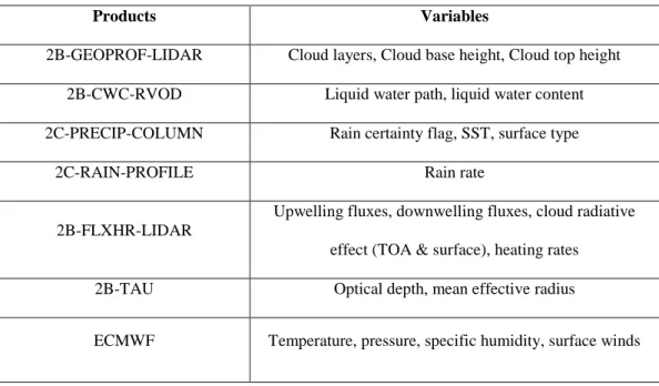
As stated previously, measurements from several CloudSat and CALIPSO data products are used to characterize the clouds in the southeast Pacific region. A number of different cloud properties are analyzed here including the vertical profile of cloud fraction, cloud top and base heights, particle effective radius, liquid water path, and optical depth. The precipitation frequency and rate is also examined to study the impacts of drizzle. Other derived products like upwelling and downwelling fluxes, radiative heating rates, and the cloud radiative effect at the top of the atmosphere are analyzed. Properties, such as temperature and moisture profiles, sea surface temperature, and lower tropospheric stability are used to characterize the environment. The CloudSat data products used in this analysis are listed in Table 1.
Table 1: Data products and variables used in research from 2007-2010
To identify low clouds, the 2B-GEOPROF-LIDAR product (Mace et al. 2009) is used. This product combines the significant echo mask from the radar-only
2B-GEOPROF retrieval product (Marchand et al. 2008) and the LIDAR vertical feature mask (Vaughan et al. 2009) to create a merged cloud mask that detects up to five cloud layers per CPR vertical profile (Mace et al. 2009). The cloud mask indicates whether each pixel detected by the CPR is either clear or cloudy by assigning a cloud probability to each of the pixels, with threshold values greater than 20 indicating a cloud (Mace et al. 2009).
To describe the characteristics of the clouds across the transition, the CloudSat 2B-TAU products are used to determine the mean cloud optical depth and effective
Products Variables
2B-GEOPROF-LIDAR Cloud layers, Cloud base height, Cloud top height 2B-CWC-RVOD Liquid water path, liquid water content 2C-PRECIP-COLUMN Rain certainty flag, SST, surface type
2C-RAIN-PROFILE Rain rate
2B-FLXHR-LIDAR
Upwelling fluxes, downwelling fluxes, cloud radiative effect (TOA & surface), heating rates 2B-TAU Optical depth, mean effective radius
radius. The optical depth of the cloud is a measure of how much radiation is able to pass through a cloud layer without getting reflected or absorbed, or how transparent a cloud is to radiation (Bodhaine et al. 1999). The geometric thickness of a cloud is related to the optical depth, where a thicker cloud will have a higher optical depth. The particle size and concentration is also a factor in determining the optical depth, as clouds with higher concentrations of large particles will result in a higher optical depth (Szczodrak et al. 2001). Also, the likelihood of precipitation may also affect the optical depth of a cloud, where heavily precipitating clouds will have a higher optical depth than
non-precipitating clouds. The 2B-TAU algorithm uses a Bayesian estimation approach (Marks and Rodgers 1993) with forward calculations to calculate the optical depth and effective radius estimates from CloudSat radar measurements, with the addition of measurements from MODIS and reanalysis data from ECMWF during the day (Polonsky 2008; Hamanda and Nishi 2010; Nakajima et al. 2010).
The CloudSat Radar-Visible Optical Depth Cloud Water Content Product (2B-CWC-RVOD) uses a forward model to retrieve estimates of the vertical profile of cloud water content for each radar profile measured by CPR (Austin et al. 2001; Marra et al. 2013). The cloud liquid water path (LWP) is calculated from 2B-CWC-RVOD as the integrated liquid water content (LWC) estimated throughout a cloud column (Wood and Taylor 2001). This product produces more accurate results than the radar only (CWC-RO) product as it uses a combination of the radar reflectivity factor from the 2B-GEOPROF product and visible optical depth estimates from the 2B-TAU product to constrain cloud retrievals more tightly (Deng 2005; Devasthale and Thomas 2012;
Rajeevan et al. 2012). One caveat is that 2B-CWC-RVOD has been shown to have significant errors in the presence of precipitation (Christensen et al. 2013). For this reason, only non-precipitating cloud LWP is analyzed in this study.
Two products from CloudSat will be used to estimate precipitation in
stratocumulus clouds in the study domain. Because the CPR is sensitive to small water droplets, even developing precipitation can be detected, which cannot be said for other spaceborne precipitation radars like the TRMM PR (Stephens and Haynes 2007). The 2C-PRECIP-COLUMN and 2C-RAIN-PROFILE are used to detect precipitation and quantify surface precipitation, respectively. The 2C-PRECIP-COLUMN product contains a precipitation flag that uses radar reflectivity thresholds to distinguish non-precipitating scenes from scenes where precipitation is possible and defines four categories: non-precipitating, rain possible, rain likely, and rain certain (Haynes et al. 2009; Lebsock et al. 2011). However, since ground clutter contaminates the bins below 720m, the 2C-PRECIP-COLUMN product has difficulty detecting rain in low-level clouds below 720 m (Rapp et al. 2013).
Whereas the 2C-PRECIP-COLUMN product identifies the likelihood of precipitation, the 2C-RAIN-PROFILE product focuses on quantitative precipitation estimation in low clouds. This product uses the CPR reflectivity profile and the path integrated attenuation (PIA), which accounts for the energy loss between the CPR and the range gate from extinction processes, to retrieve the vertical distribution of rainwater (Mitrescu et al. 2010; Lebsock and L’Ecuyer 2011) and contains several improvements over the early quantitative estimates of precipitation by CloudSat. This retrieval product
includes a visible optical depth constraint from MODIS, a model for the evaporation of rain that occurs directly beneath the cloud layer (similar to a model from Comstock et al. 2004), and raindrop size distributions that are more representative of warm rain
processes (Lebsock and L’Ecuyer 2011). These improvements are especially important for boundary layer clouds in this region and validation against in situ radar estimates shows generally good agreement (Rapp et al. 2013).
Because the radiative feedbacks are so important to the development and maintenance of stratocumulus and shallow cumulus clouds and top of atmosphere shortwave cloud forcing is so important for capturing climate sensitivity, this study uses the new 2B-FLXHR-LIDAR product which incorporates measurements from the CPR, CALIPSO, and MODIS to estimate the broadband fluxes and heating rates for each CloudSat radar profile along the trajectory. The 2B-FLXHR-LIDAR product builds off the 2B-FLXHR approach, but the revised product also makes use of the CALIPSO vertical feature mask through CloudSat's 2B-GEOPROF-LIDAR product (Mace 2007; Marchand et al. 2008) to detect low clouds missed by CloudSat. The cloud radiative effect on the shortwave fluxes at the top of the atmosphere (TOA_CRE) in the shortwave is calculated by determining the difference between clear and cloudy
conditions (Charlock and Ramanathan 1985; Hartmann et al. 1986). The rate of radiative heating is determined by calculating the amount of flux that is either absorbed or emitted within each cloud layer in the vertical profile.
The ECMWF-AUX uses environmental profiles of pressure, temperature, and specific humidity from European Center for Medium-Range Weather Forecasting
(ECMWF) analyses, which are then interpolated to each CloudSat vertical bin (Lebsock and L’Ecuyer 2011). The importance of these variables is highlighted in Figure 1 as each variable influences the formation and development of marine stratocumulus clouds and could play a leading role in the transition to cumulus clouds. There are some
shortcomings with using reanalysis data, however, where the data from ECMWF is comprised of analysis data that is only updated every 6-12 hours and is prone to biases due to inadequate vertical resolution (Yue et al. 2013).
2.2 Methods
The area of interest for this study is the southeast Pacific Ocean (SEP).
Specifically, this study examines low-level clouds on a 2° x 2° grid from 30°S-5°N and from 85°W-110°W, excluding any cloudy scenes over land. These boundaries were chosen because they not only encompass the climatological trajectories from Sandu et al. (2010), but also because of the number of recent field campaigns studying the marine stratocumulus clouds that dominate this region. Unlike scanning instruments like MODIS, CloudSat’s non-scanning nadir-viewing CPR limits with the number of times the study region is sampled both day and night, so longer temporal averaging is
necessary to collect enough observations for an accurate representation of the region for this analysis. Rapp et al. (2014) found that the spacing of the grid boxes allows for the optimal representation of the climatological representation because any smaller sized grid boxes would result in more noise in the data collected and if the grid boxes were larger, the structure of the clouds and localized effects along the trajectory would be
missed. Therefore, this study analyzes satellite data from 1 January 2007 to 31 December 2010 to aggregate enough observations to develop a more complete representation of cloud properties, precipitation, and radiative effects of this cloud system. This analysis will provide a detailed description of the climatological cloud, precipitation, and radiative characteristics across the transition in low-level
stratocumulus clouds as they break up into cumulus clouds in the southeast Pacific.
2.2.1 Low cloud identification
First, the four years of CloudSat, CALIPSO, and environmental data are extracted from the files listed in Table 1 and processed within the southeast Pacific region defined above. For this analysis, a profile is considered cloudy if there is at least one cloud layer detected in 2B-GEOPROF-LIDAR. Since this study is only interested in stratocumulus and shallow cumulus low-level clouds, the analysis is limited profiles with cloud heights below 4 km. This boundary is chosen because stratocumulus clouds rarely exceed 2 km; however, convective shallow cumulus can penetrate through this low cloud layer (Comstock et al. 2005) and disorganized shallow cumulus cloud heights increase as the boundary layer deepens near the equator (Bretherton et al. 2003). For this analysis, cloudy scenes where only a single layer of clouds is detected from the CPR are the primary data source. One problem that may arise from the use of single layer clouds is the contamination of overlying cirrus clouds, with its impact felt most near the equator where deep convection is more prominent. The overlying cirrus associated with anvils
from deep, convective clouds along the Intertropical Convergence Zone (ITCZ) will impact our ability to capture the full effect of the shallow cumulus clouds.
2.2.2 Cloud, radiative, and environmental properties
To understand the macrophysical and microphysical cloud characteristics of stratocumulus as they transition into shallow cumulus clouds, the CloudSat GEOPROF-LIDAR, TAU, and CWC-RVOD products are used. The
2B-GEOPROF-LIDAR retrieves up to five cloud layers in each vertical profile (Mace et al. 2009). If at least one cloud layer is detected and the cloud top height of the highest layer falls below the 4 km boundary set for this study, the cloud layer base and top height are recorded and the profile containing low clouds is analyzed. The profiles that meet these criteria are then used to calculate the low cloud fraction, which is important for
analyzing how the macrophysical structure of the stratocumulus cloud system changes as they break apart into shallow cumulus clouds. The cloud fraction for a given level in the vertical profile is defined as the number of cloud observations detected within a cloud layer divided by the total number of observations in that cloud layer. To calculate the total grid box cloud fraction, the total number of cloud observations within a grid box is divided by the total number of observations in that grid box.
Because the presence of precipitation leads to overestimations in some variables (Wood 2008), only cloud variables from 2B-CWC-RVOD and 2B-TAU that contain no precipitation are analyzed. The mean liquid water path is calculated as the sum of all valid liquid water path retrievals divided by the number of cloud observations in that grid box. The mean optical depth and effective radius follow the same process as the
calculation for the LWP, where the total of the values for each variable in that grid box is divided by the number of cloud observations in that grid box. Because the retrieval of effective radius and optical depth require MODIS visible reflectances, they are only calculated during the day, whereas the mean LWP is calculated both day and night since it can be retrieved solely from the CPR reflectivity profiles.
To study precipitation across the transition, the CloudSat 2C-RAIN-PROFILE near-surface precipitation estimate and the 2C-PRECIP-COLUMN precipitation occurrence flag are used. For this analysis, the confidence flag from
2C-PRECIP-COLUMN is used to calculate the frequency of precipitation. The confidence flag ranges from no precipitation detected (when the precipitation flag (pflag) = 0) to certain rainfall detected (pflag = 3). To test the sensitivity of the confidence flag, we compare the frequency of whenever rainfall is possible (pflag = 1) to when rainfall is certain (pflag = 3). The frequency of precipitation in both cloudy scenes and in all (cloudy sky + clear sky) scenes is calculated as the total number of times precipitation with a given confidence flag (either 1 or 3 in this case) divided by either the total number of
observations in that grid box or the total number of cloud observations detected in that grid box. The rain rate retrieval from the 2C-RAIN-PROFILE quantifies the intensity of drizzle. Clouds are considered to be precipitating when the 2C-PRECIP-COLUMN identifies a profile as ‘rain certain’ and the 2C-RAIN-PROFILE has a rainfall rate greater than zero. This analysis considers both the conditional and unconditional rain rate. The unconditional rain rate is the sum of all values of rainfall intensity divided by the total number of observations from each grid box. The conditional rain rate is
calculated from the sum of the estimated rainfall intensity and divided by the total number of precipitating observations in that grid box.
Cloud top longwave cooling is important for the development and maintenance of stratocumulus and has been found to strongly influence the turbulence that occurs within the stratocumulus cloud layer (Bretherton et al. 2010). Shortwave heating rates during the day are also important since they describe the absorption that occurs at the top of the cloud layer, which helps to break up the clouds. The cloud radiative effect in the shortwave is important for understanding the radiative impact clouds have on the top of the atmosphere and how they influence Earth’s radiation budget (Charlock and
Ramanathan 1985). The 2B-FLXHR-LIDAR product is used to examine the longwave and shortwave heating rates, as well as upwelling and downwelling fluxes, paying special attention to the cloud top longwave cooling across the transition and the shortwave radiative impact of clouds. The amount of cooling at the cloud top is calculated by dividing the sum of all longwave cooling rates from each cloud top observation by the total number of cloud observations. The same process is repeated for the shortwave heating at the cloud top; however, only daytime scenes are considered. The shortwave TOA_CRE is calculated from the difference in radiative fluxes between cloudy conditions and clear-sky conditions (Hartmann et al. 1986).
The environmental profiles are important to examine as the clouds advect equatorward where waters are warmer and shallow convection is more favorable. The temperature and humidity profiles describe the structure of the boundary and inversion layers as they evolve throughout the transition process. Surface wind, relative humidity,
and surface temperature help to improve the understanding of the environment at the surface by determining the surface latent heat flux, which is the key source of moisture to the lower level clouds (Hartmann 1994; Wood 2012). To describe the thermodynamic conditions across the transition, the ECMWF-AUX product is used, which provides atmospheric temperature, pressure, and humidity profiles, as well as the surface wind speed and the sea surface temperatures from the ECMWF analyses that have been collocated with CloudSat. It should be noted here that the data from ECMWF is comprised of analysis data that is only updated every 6-12 hours and is prone to biases (Yue et al. 2013); however, this dataset provides the most complete representation of the clouds’ environment given the lack of actual observations available for this analysis. To calculate the mean atmospheric profiles in the study, the environmental data is summed over each level in the vertical profile between the surface and 4 km and then divided by the total number of observations for each vertical profile layer.
Lower tropospheric stability (LTS) is a measure of strength of the inversion layer found above the boundary layer where stratocumulus clouds develop (Wood and Hartmann 2006). LTS, shown in Equation (1), is the difference between the potential temperature the 700mb level, or free troposphere, and the surface (Slingo 1987; Klein and Hartmann 1993). Similar to the other variables, the mean LTS is calculated as the sum of all cloud observations within each grid box divided by the total number of cloud observations in that box.
2.2.3 Climatological trajectory analysis
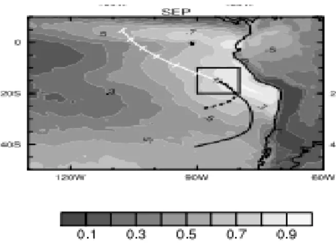
Using the 4-year dataset developed for the larger southeastern Pacific domain, we follow an approach similar to Sandu et al. (2010) and analyze data along the
climatological trajectory locations described in the appendix of their paper. Sandu et al. (2010) showed that the spatial structure of the climatological trajectories capture the evolution of the airmasses and are therefore, useful for studies on the transition from stratocumulus to shallow cumulus clouds. Figure 5 from Sandu et al. (2010) illustrates the medians of selected forward and backward trajectories calculated in the southeast Pacific Ocean. Figure 6 shows the points that were calculated along the trajectory after a linear fit between the coordinates from Sandu et al. (2010). Because of CloudSat’s near-nadir only sampling, 2x 2boxes are defined around each of our trajectory data points in Figure 6 to aggregate enough data for the climatological representation of the clouds throughout the transition. The asterisks are trajectory points used for this study and the plus signs are the data trajectory points from Sandu et al. (2010). The lines found on each side of the data points in Figure 6 represent the endpoints for the 2x 2boxes used in this study. Data in each of these grid boxes is analyzed throughout the 4-year period to characterize the climatology and interannual variability in cloud properties, precipitation, and radiation effects along the climatological transition trajectory. Table 2 lists the coordinates along the trajectory and the total number of observations for the four-year period in each coordinate grid box.
Figure 5: Cloud fraction on the third day of the selected trajectories, and medians of the forward (white line) and the backward (black line) climatological trajectories in the southeast Pacific and Atlantic Oceans. (Sandu et al. 2010)
Figure 6: Trajectory coordinate points (*) with the 2x 2boxes around each of the trajectory data points (*).The other points (+) are trajectory points calculated from the Appendix of Sandu et al. (2010).
Latitude Longitude Total # of Observations -85.000 -15.000 36533 -87.000 -13.608 28803 -89.000 -12.231 35743 -91.000 -11.096 35020 -93.000 -9.864 43615 -95.000 -8.577 41926 -97.000 -7.431 33146 -99.000 -6.001 32722 -101.000 -4.106 28847 -103.000 -0.625 32335 -105.000 1.882 42628
Table 2: List of coordinate points used in study and the total number of observations collected within each 2x 2box around each coordinate.
The annual mean climatology of each variable is computed for each of the 4 years to observe the mean key features of stratocumulus clouds and shallow cumulus clouds. The interannual variability is then analyzed by comparing the 4 years to each other to distinguish any major differences between the years. It is important to examine the year-to-year fluctuations for the different cloud, environmental, and radiative variables for any distinctive features in particular years that differ from the four-year mean pattern. Because there is a large seasonal cycle in cloud amount (Klein and Hartmann 1993), data is analyzed seasonally by grouping the data in three-month
periods for all years to describe the intraseasonal variability in transition features. To represent each season for all years, the months are grouped together as March/April/ May (MAM), June/July/August (JJA), September/October/November (SON) and December/January/ February (DJF).
Cloud fraction and precipitation have also been shown to peak during the nighttime and early morning hours (Klein et al. 1995; Rapp et al. 2013), so analysis of the diurnal variability in cloud properties across the stratocumulus to cumulus transition is also performed. For this analysis, the data is divided at 1200 UTC, near sunrise. Thus, anything before 1200 UTC is considered night and anything after 1200 UTC is
considered day. It should be noted that this analysis does not represent the full diurnal cycle, but rather represents the day/night differences between observations at the CloudSat overpass times, which occur in the very early morning and early afternoon.
3. RESULTS
3.1 Climatological representation
The four-year means calculated along the climatological trajectory for each of the variables are first investigated. The first variables discussed are the atmospheric profiles, followed by the cloud properties, precipitation, and finally, the radiative variables.
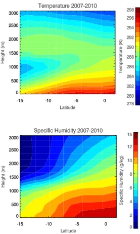
The four-year mean climatology of the environmental profiles up to 3 km is shown in Figure 7a-d. The SSTs in Figure 7a show an overall increase in temperatures as the trajectory moves equatorward. Just south of the equator, temperatures decrease because of the equatorial cold tongue, a feature where enhanced mixing from the equatorial currents and horizontal large-scale wind patterns cause a significant drop in the SSTs (Wallace et al. 1989; Moum et al. 2013). The corresponding atmospheric temperature profile is shown in Figure 7b with near-surface values ranging from 290 K at 15S to 296 K near the equator. A temperature inversion is present between 1.1 - 1.5 km and is strongest in the southern region where the mean inversion in the ECMWF analysis is about 4 K. The inversion strength in this study is likely underestimated based on in situ results from previous studies that have shown the low vertical resolution in models and reanalysis (Rahn and Garreaud 2011) leads to underestimates of the
inversion strength. The lower tropospheric stability (LTS) is shown in Figure 7c with the greatest stability at the southernmost point of the trajectory and decreasing stability approaching the equator, due to the deepening boundary layer and increased SSTs. The specific humidity in Figure 7d features the greatest humidity near the surface in the
northern portion of the study region and lowest values of moisture above the boundary layer in the southernmost portion of the study region. A stronger vertical gradient is noticeable at the top of the boundary layer farther south where cool and dry, subsiding air is present and the temperature inversion is much stronger (Norris and Klein 2000).
(A) (B)
(C) (D)
Figure 7: Four-year mean representation of the environmental variables (a) SST in °C (b) temperature profile (K), (c) the LTS (K), and (d) specific humidity (g kg-1), along the climatological wind trajectory in
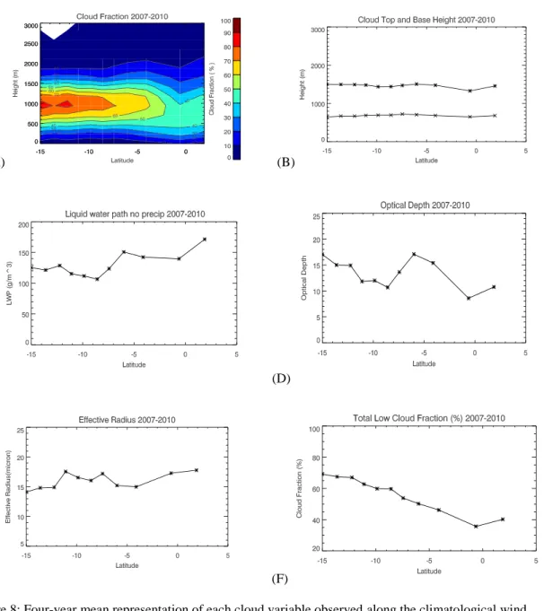
The four-year means for each of the cloud variables are shown in Figure 8a-e. The vertical profile of cloud fraction below 3 km in Figure 8a shows that the greatest percentage of clouds is located around 1 km, with higher values are seen in the southernmost grid boxes where persistent stratocumulus cloud decks are commonly located. The fraction of clouds decreases throughout the vertical profile just south of the equator indicating the transition to a shallow cumulus regime. To facilitate comparison with past studies using other non-profiling instruments, the total low cloud fraction, defined as the total number of cloud observations divided by the total number of observations in a grid box, is shown in Figure 8f. Again, it shows a gradual decline in low clouds over the transition, with a minimum located just south of the equator. The single layer cloud top and base heights in Figure 8b show relatively constant mean heights along the trajectory, with only a small dip in the cloud top height. Cloud top heights for the single layer are normally around 1.5 km with the lowest value around 1.4 km whereas the cloud base heights remain constant around 0.65 km. The reduction in cloud fraction just south of the equator is likely due to the equatorial cold tongue positioned off the Peruvian coastline where lower SSTs are found in contrast to the higher SSTs throughout the tropical regions (Mansbach and Norris 2007). The strong temperature inversion and increased LTS values in the southernmost portion of the study region correspond well with the greater cloud fractions. As the trajectory approaches the equator, SSTs are warmer and the subsidence is reduced, causing a weakening in the inversion as the stratocumulus cloud decks break apart and allow convective shallow cumulus with lower cloud fraction to dominate the region. Near the equator the breakup
of the stratocumulus deck from the weaker subsidence and inversion layer is evident as the cloud fractions drop considerably, but the fraction of deeper, more convective clouds increases. The average change in the low cloud fraction from the peak and minimum amount of clouds is also calculated to consider the speed of the transition period and how it varies along the trajectory from year to year. A steady reduction in the total low cloud fraction is observed throughout most of the trajectory, however the minimum in cloud fraction varies between 10° S and 5°S interannually as this region is where the low cumulus clouds develop under the thinning stratocumulus deck. The speed of the
transition changes rapidly around 5°S as cumulus clouds develop more near the ITCZ, as shown in the low cloud fraction climatology. A number of factors play a role in where the minimum amount of clouds occurs along the trajectory, as the time it takes the transition from stratocumulus to cumulus may vary from year to year.
The next three figures are closely related to one another, as the optical depth of a low cloud is proportional to the LWP and inversely related to the effective radius
(Stephens et al. 1978). Figure 8c shows the LWP for non-precipitating clouds, where the four-year mean LWP values are between 100-175 mg m-3. There are lower LWPs in the southern coordinate points that increase closer to the equator, with the higher LWP values around 5°S closely corresponding to the increased amount of deeper clouds seen in Figure 8a-b. The optical depth in Figure 8d varies along the trajectory with the highest values of about 17 found at 15°S and 4°S and the lowest value of about 9 just south of the equator. The trends found in the optical depth are also evident in the cloud fraction in Figure 8a where values of optical depth on average are lower close to the equator and
highest near the southern boundary of the study region. The effective radius in Figure 8e ranges from 14-18 μm throughout the trajectory.
(A) (B)
(C) (D)
(E) (F)
Figure 8: Four-year mean representation of each cloud variable observed along the climatological wind trajectory in the southeast Pacific. The panels are (a) cloud fraction (%), (b) cloud layer top and base heights (m), (c) optical depth during the day (unitless), (d) effective radius during the day (microns), (e) non-precipitating cloud liquid water path (g m-2), and (f) total low cloud fraction (in %).
The greatest variability in the effective radius, cloud fraction, and other
environmental variables is found between 12°S and 6°S, likely due to the transition that takes place as the large scale subsidence decreases, the inversion layer begins to weaken, and the shallow cumulus clouds begin to develop beneath the dissipating stratocumulus cloud deck as the boundary layer weakens and deepens. The overall trend is a slight increase in effective radius and liquid water path toward the equator. The optical depth features more noise compared to the previous two variables, but increased close to the equator where the cloud layer is thicker and LWP values are greater. Both the effective radius and the optical depth are retrieved similarly using radar reflectivity (Polonsky et al. 2008), therefore changes in these variables should in turn affect the LWP. There appear to be inconsistencies between the mean cloud optical depth, LWP, and effective radius near the equator; however, the effective radius and optical depth are not retrieved at night, unlike LWP. At night LWP is retrieved without the optical depth constraint, therefore, the results for the optical depth and effective radius do not follow the expected relationship with LWP.
Another potential limitation of using CloudSat-retrieved properties is that the CPR is unable to detect clouds in the lowest 2-3 bins because of ground clutter; therefore, when cloud bases extend below about 720 m, retrieved integrated quantities like LWP and optical depth may be underestimated. The cloud fraction in Figure 8a shows where some of the greatest impacts are likely, as clouds, though fewer, are often found below 720 m near to the equator. To verify the CloudSat retrievals, a brief
comparison of the LWP, effective radius, optical depth, and cloud fraction
climatological results to the level 3 MODIS (MOD08_M3.051) products was performed (not shown). Overall, the MODIS retrievals for optical depth, effective radius, and LWP show general agreement between the cloud variables, as MODIS values for the effective radius are lower on average than the CloudSat retrievals but only by about 10 %,
although MODIS values are significantly lower for the LWP and optical depth, with a difference greater than 30 %. A lack of agreement between MODIS and CloudSat retrievals is found around 6°S where a significant increase in LWP and optical depth is not detected by MODIS, but it is likely not an artifact because in this area, the SST is relatively high and there is more frequently occurring shallow convection, resulting in an increase in LWP and optical depth. The MODIS products used for comparison also did not have the 4 km cloud top height, single layer, and non-precipitating restrictions, which could also account for some of these differences.
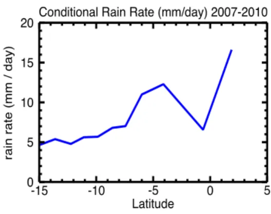
The four-year mean climatology for the rain frequency and rain rate for all observations are shown in Figure 9a and 9b, respectively. The rain possible frequency for cloudy scenes (blue line) is the likelihood that radar reflectivity is between 15 and -7.5 dBz, whereas the rain certain frequency for cloudy scenes is the likelihood that radar reflectivity is greater than 0 dBz. Precipitation in clouds with tops less than 4km is more frequent in the southern portion of the study area, with rain possible in nearly 30% of observations at 15°S. Values decrease as the trajectory approaches the equator and reach a minimum just south of the equator due to the lower occurrence of clouds observed in Figure 8a as the stratocumulus cloud deck advects equatorward over the SST cold