The Analog Data Assimilation
REDOUANELGUENSAT ANDPIERRETANDEO
IMT Atlantique, Lab-STICC, UniversitéBretagne Loire, Brest, France PIERREAILLIOT
Laboratoire de Mathématiques de Bretagne Atlantique, University of Western Brittany, Brest, France MANUELPULIDO
Department of Physics, Universidad Nacional del Nordeste, and CONICET, Corrientes, Argentina RONANFABLET
IMT Atlantique, Lab-STICC, UniversitéBretagne Loire, Brest, France
(Manuscript received 23 November 2016, in final form 31 July 2017) ABSTRACT
In light of growing interest in data-driven methods for oceanic, atmospheric, and climate sciences, this work focuses on the field of data assimilation and presents the analog data assimilation (AnDA). The proposed framework produces a reconstruction of the system dynamics in a fully data-driven manner where no explicit knowledge of the dynamical model is required. Instead, a representative catalog of trajectories of the system is assumed to be available. Based on this catalog, the analog data assimilation combines the nonparametric sampling of the dynamics using analog forecasting methods with ensemble-based assimilation techniques. This study explores different analog forecasting strategies and derives both ensemble Kalman and particle filtering versions of the proposed analog data assimilation approach. Numerical experiments are examined for two chaotic dynamical systems: the Lorenz-63 and Lorenz-96 systems. The performance of the analog data assimilation is discussed with respect to classical model-driven assimilation. A Matlab toolbox and Python library of the AnDA are provided to help further research building upon the present findings.
1. Introduction
The reconstruction of the spatiotemporal dynamics of geophysical systems from noisy and/or partial observa-tions is a major issue in geosciences. Variational and stochastic data assimilation schemes are the two main categories of methods considered to address this issue [seeEvensen (2007)for more details]. A key feature of these data assimilation schemes is that they rely on re-peated forward integrations of an explicitly known dy-namical model. This may greatly limit their application
range as well as their computational efficiency. First, thorough and time-consuming simulations may be required to identify explicit representations of the dynamics, especially regarding finescale effects and subgrid-scale processes as for instance in regional geo-physical models (Hong and Dudhia 2012). Such pro-cesses typically involve highly nonlinear and local effects (Wilby and Wigley 1997). The resulting numer-ical models may be computationally intensive and even prohibitive for assimilation problems, for instance re-garding the time integration of members with different initial conditions at each time step. Second, as explained in Van Leeuwen (2010), ‘‘with ever-increasing resolu-tion and complexity, the numerical models tend to be highly nonlinear and also observations become more complicated and their relation to the models more nonlinear’’ (p. 1991). In such situations, standard data assimilation techniques may find difficulties, including
Supplemental information related to this paper is avail-able at the Journals Online website: https://doi.org/10.1175/ MWR-D-16-0441.s1.
Corresponding author: Redouane Lguensat, redouane.lguensat@ imt-atlantique.fr
DOI: 10.1175/MWR-D-16-0441.1
2017 American Meteorological Society. For information regarding reuse of this content and general copyright information, consult theAMS Copyright Policy(www.ametsoc.org/PUBSReuseLicenses).
nonlinear particle filters which are prone to the ‘‘curse of dimensionality.’’ Third, difficulties may occur when geophysical dynamics involve uncertain model param-eterizations or space–time switching between different dynamical modes that need to be estimated online (Ruiz et al. 2013) or offline (Tandeo et al. 2015b). Dealing with such situations may not be straightforward using classi-cal model-driven assimilation schemes.
Meanwhile, recent years have witnessed a prolifera-tion of satellite data, in situ monitoring, as well as numerical simulations. Large databases of valuable information have been collected and offer a major opportunity for oceanic, atmospheric, and climate sci-ences. As pioneered byLorenz (1969), the availability of such datasets advocates for the development of analog forecasting strategies, which make use of ‘‘similar’’ states of the dynamical system of interest to generate realistic forecasts. Analog forecasting strategies have become more and more popular in oceanic and atmo-spheric sciences (Nagarajan et al. 2015;McDermott and Wikle 2016), and have benefited from recent advances in machine learning (Zhao and Giannakis 2014). They have been applied to a variety of systems and applica-tion domains, including among others, rainfall now-casting (Atencia and Zawadzki 2015), air quality analysis (Delle Monache et al. 2014), wind field down-scaling (He-Guelton et al. 2015), climate reconstruction (Schenk and Zorita 2012), and stochastic weather gen-erators (Yiou 2014).
In this work, we examine the extension of the analog forecasting paradigm for data assimilation issues. Given a representative dataset of the dynamics of the system, this extension that we call analog data assimi-lation (AnDA) consists of a combination of the implicit analog forecasting of the dynamics with stochastic fil-tering schemes, namely, ensemble Kalman and particle filtering schemes (Evensen and Van Leeuwen 2000). This idea was first introduced inTandeo et al. (2015a)
where the relevance of the proposed analog data as-similation is shown for the reconstruction of complex dynamics from partial and noisy observations. Tandeo et al. derived filtering and smoothing algorithms called theanalog ensemble Kalman filter and smoother, which combine analog forecasting and the ensemble Kalman filter and smoother. A similar philosophy was followed independently inHamilton et al. (2016)where the au-thors combine ideas from Takens’s embedding theorem and ensemble Kalman filtering to infer the hidden dy-namics from noisy observations. Hamilton et al. called their algorithm theKalman–Takens filter.
Whereas these two previous works provide proofs of concept, our study further investigates and evaluates different analog assimilation strategies and their detailed
implementation. Our contributions are threefold. First, we present and examine various analog forecasting strategies, including locally linear ones that were not considered in previous works, and evaluate their performance for analog data assimilation. Second, in addition to the ensemble Kalman algorithms, we propose and examine a novel implementation of the analog forecasting combined with a particle filter. Finally, in the online supplemental material, we provide a unified computational framework, through both a Matlab Toolbox and a Python Library, to pave the way for practical use and future research (https://github. com/ptandeo/AnDA).
The work is organized as follows. In section 2, we briefly present the general concepts of data assimilation and introduce the key ideas of analog data assimilation. Different analog forecasting strategies are introduced in
section 3.Section 4describes the different components of the proposed analog data assimilation framework and the associated algorithms. Numerical experiments for two classical chaotic dynamical systems are reported in
section 5.Section 6 further discusses our work, high-lights our key contributions, and proposes possible di-rections for future work.
2. General context
a. Model-driven data assimilation
Classically, data assimilation is based on the following discrete state space (Bocquet et al. 2010):
x(t)5M[x(t21),h(t)], (1)
y(t)5H[x(t)]1«(t) , (2) where timet2 f0,. . .,Tgrefers to the times in which observations are available. For the sake of simplicity we assume observations are at regular time steps.
In(1),M characterizes the dynamical model of the true state x(t), while h(t) is a random perturbation added to represent model uncertainty. The observation equation (2) describes the relationship between the observation y(t) and x(t). Observation error is consid-ered through the random noise«(t). Here, for the sake of simplicity, we consider an additive Gaussian noise«with covarianceRin(2)and the observation operatorH5H is assumed linear.
Data assimilation aims to reconstruct the state se-quencefx(t)gfrom a series of observationsfy(t)g. Two types of data assimilation schemes are extensively studied in the literature: variational and stochastic. Variational data assimilation proceeds by minimizing a cost function based on a continuous formulation of(1) and (2)(see
schemes rely on the sampling and/or maximization of the posterior likelihood of the state sequence given the ob-servation series (seeKalnay 2003). These classical data assimilation schemes are regarded as ‘‘model driven,’’ in the sense that they combine observations with forecasts provided by a numerical modelM.
b. Data-driven data assimilation
The proposed assimilation framework relies on a similar state-space formulation. The key feature is to substitute the explicit dynamical modelM in(1)by a ‘‘data driven’’ dynamical model involving an analog forecasting operator, denoted byA, namely,
x(t)5A[x(t21),h(t)]. (3) Henceforth, this state-space model will be referred to as AnDA. A sequential and stochastic data assimilation scheme including filtering and smoothing, is used in-volving different Monte Carlo realizations of the state at each assimilation time. We sketch the proposed AnDA methodology for one realization inFig. 1.
The analog forecasting operator Arequires the ex-istence of a representative dataset of exemplars of the considered dynamics. This dataset is referred to as the
catalog and denoted by C. The reference catalog is formed by pairs of consecutive state vectors, separated by the same time lag. The second component of each pair is referred to as the successor of the first component hereafter. The catalog may be issued from observational data as well as from numerical simulations. In the last case, one can have a catalog issued from numerical simulations (based on physical equations), and wants to perform data assimilation without running the model
again. This is for instance useful for operational pdiction centers that do not have the computational re-sources to integrate a forecast model, but do have access to a large database of numerical simulations or analysis data of a large prediction center. In this respect, we discuss also the situation where the catalog comprises noisy versions of the true states (section 5d).
Given a catalogC, the analog forecasting operatorA is stated as an exemplar-based statistical emulator of the state x from time t to time t1dt. For any state x(t), we emulate the following state at timet1dtbased on its nearest neighbors in catalog C. Given the analog forecasting operator, we present associated stochastic assimilation schemes, namely the analog ensemble Kalman filter/smoother (Tandeo et al. 2015a) and the
analog particle filter.
3. Analog forecasting strategies a. Analog forecasting operator
Let us consider a kernel function, denoted byg, in the state space (Schölkopf and Smola 2001). Among the classical choices for kernels, we consider here a radial basis function (also referred to as a Gaussian kernel):
g(u,y)5exp(2lku2yk2) , (4) wherelis a scale parameter, (u,y) are variables in the state spaceX, andk.kis the Euclidean distance or an-other appropriate distance function. Note that the pro-posed analog forecasting operator may be applied to other kernels or subspace reduction methods to effi-ciently retrieve relevant analog situations. This is dis-cussed insection 6.
Given the considered kernel, the analog forecasting operatorAis defined as follows: for a given statex(t), we denote byak[x(t)] itskth nearest neighbor (or analog situation) in the reference catalog of exemplarsC, and bysk[x(t)] the known successor of stateak[x(t)]. Here-inafter, we refer byKto the number of nearest neigh-bors (analogs), and by covwthe weighted covariance. The normalized kernel weight for every pairfak[x(t)],sk[x(t)]g is given by vk[x(t)]5 gfx(t),ak[x(t)]g
K K51 gfx(t),ak[x(t)]g . (5)Several ideas can be explored to define the analog forecasting operatorA. The natural first option consists in deriving the forecast using the weighted mean of the
Ksuccessors. This approach, that we call here thelocally constant operator, was considered in many analog forecasting related works (McDermott and Wikle 2016;
FIG. 1. The evolution in time of one particle or member. The catalog implicitly represents the dynamics of the system from ex-emplars of historical datasets. The observations are shown by black asterisks, and their variance is shown by the corresponding error bar.
Zhao and Giannakis 2014;Hamilton et al. 2016), and is also known in statistics as Nadaraya–Watson kernel regression. One can also use as analog forecasting op-erator the weighted mean of the anomalies between the
Kanalogs and their successors and adding it to the state to derive the forecast. The operator, referred to as lo-cally incremental, is seen as more physically sound and relates more closely to a finite-difference approximation of the underlying differential equations. Finally, we in-troduce in this work a new analog forecasting operator that makes use of local linear regression techniques based on weighted least squares estimates. This operator that we call thelocally linearoperator is known to make an efficient use of small datasets and to reduce biases (Cleveland 1979). Note that the locally constant and locally incremental operators are two special cases of the locally linear operator.
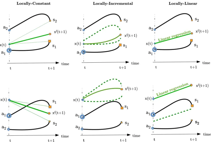
Figure 2 shows an illustration of the three analog forecasting operators used in this work. Hereafter, we denote the forecasted state asxf(t1dt). The three an-alog forecasting operators are defined as follows for two
sampling schemes: a Gaussian sampling and a multino-mial one. Hereinafter, dZ() denotes a delta function centered onZ.
d Locally constant analog operator: for the Gaussian case, the forecasted state is sampled from a Gaussian distribution whose meanmLCand covarianceSLCare the weighted mean and the weighted covariance estimated from theKsuccessors and their weights:
xf(t1dt);N (mLC,SLC), (6)
where mLC 5
K
k51vk[x(t)]sk[x(t)] and SLC 5 covv(sk[x(t)]k2〚1,K〛). While in the multinomial case, the forecasted state is drawn from the multinomial discrete distribution that samples the successorsk[x(t)] with a probability ofvk: xf(t1dt);
K k51 vk[x(t)]ds k[x(t)]() . (7)d Locally incremental analog operator: instead of considering a weighted mean of the Ksuccessors as
FIG. 2. A simplified illustration of the considered analog forecasting strategies in the case of two analogs (nearest neighbors). Two situations for the statex(t) are shown: (top) a situation wherex(t) lies in the convex hull spanned by catalog exemplars and (bottom) a situation wherex(t) lies farther from its analogs. The second situation is expected to occur more often for high-dimensional space as well as for states, which are less likely. The latter may model extreme events or outliers.
in the locally constant operator, we consider the value of the current state plus a weighted mean of theK
incrementstk, that is, the differences between ana-logs and successors tk[x(t)]5sk[x(t)]2ak[x(t)]. The Gaussian sampling is given by
xf(t1dt);N (mLI,SLI), (8) where mLI 5 x(t) 1
K k51vk[x(t)]tk[x(t)] 5 K k51vk[x(t)]fx(t) 1 tk[x(t)]g and SLI 5 covv(fx(t) 1 tk[x(t)]gk2〚1,S〛) and the multinomial sampling resorts to xf(t1dt); K k51 vk[x(t)]dx(t)1t k[x(t)]() . (9)d Locally linear analog operator: we fit a multivari-ate linear regression between the K analogs of the current state and their corresponding successors us-ing weighted least squares estimates (seeCleveland 1979). The regression gives slope a[x(t)] and inter-cept b[x(t)] parameters, and residuals jk[x(t)] 5
sk[x(t)]2(a[x(t)]ak[x(t)] 1 b[x(t)]). The Gaussian sampling comes to
xf[(t1dt)];N (m
LL,SLL), (10)
with mLL 5 a[x(t)]x(t) 1 b[x(t)] and SLL 5 cov(jk[x(t)]k2〚1,K〛), while the multinomial sampling is given by xf(t1dt);
K k51 vk[x(t)]dm LL1jk[x(t)]() . (11)The choice of one operator over another depends mostly on the available computational resource and the complexity of the application. Locally constant and lo-cally increment operators are less time and memory consuming than the locally linear operator, and while they can be of comparable performance in case of a flat regression function, the locally linear is expected to better deal with curvier regression functions at the ex-pense, however, of the requirement of a larger number of analogs to fit the regression (Hansen 2000). The lo-cally linear and the lolo-cally incremental are more suitable for samples near or outside the boundary of the select analogs (as depicted inFig. 2), this may be particularly relevant in geoscience applications where chaos and extreme events are of high interest.
b. Global and local analogs
The global analog strategy is the direct application of the introduced analog forecasting strategies to the entire state vector. We also introduce a local analog fore-casting operator. For a given state x(t), the analogs
ak[xl(t)] in the reference catalog, and their associated
successors sk[xl(t)] for each component l of the state
x(t) are defined according to a component-wise local neighborhood, typically fxl2n(t),. . .,xl(t),. . .,xl1n(t)g with n being the width of the considered component-wise neighborhood, such that the evaluation of the kernel function and the computation of the associated normalized weights vk[xl(t)] only involve this local neighborhood.
The idea of using local analogs is motivated by the fact that points tends to scatter far away from each other in high dimensions, which make the search for skillful an-alogs nearly impossible for high-dimensional state space. For instance, Van den Dool (1994) has shown that finding a relevant analog at synoptic scale over the Northern Hemisphere for atmospheric data would re-quire 1030 years of data to match the observational errors at that time. Conversely, analog forecasting schemes may only apply to systems or subsystems as-sociated with low-dimensional embedding. Following this analysis, the analog forecasting of the global state is split as a series of local and low-dimensional analog forecasting operations. Note that such local analogs also reduce possible spurious correlations.
4. Analog data assimilation
The analog data assimilation is stated as a sequential and stochastic assimilation scheme, using Monte Carlo methods. It amounts to estimating the so-called filter-ing and smoothfilter-ing posterior likelihoods, respectively,
p[x(t)jy(1),. . .,y(t)] the distribution of the current state knowing past and current observations and
p[x(t)jy(1),. . .,y(T)] the distribution of the current state knowing past, current, and future observations. We investigate both ensemble Kalman filter/smoother and particle filter.
a. Analog ensemble Kalman filter and smoother (AnEnKF/AnEnKS)
Ensemble Kalman filters (EnKF) and smoothers (EnKS) (Burgers et al. 1998;Evensen 2007) are partic-ularly popular in geoscience as they provide flexible assimilation strategies for high-dimensional states. They rely on the assumption that the filtering and smoothing posteriors are multivariate Gaussian distributions, such that the following forward and backward recursions are derived. The next two paragraphs present the AnEnKF and AnEnKS equations, which are equivalent to those of the EnKF and EnKS described in Tandeo et al. (2015b), except for the update step where we use the analog forecasting operator.
The forward recursions of the AnEnKF correspond to the stochastic EnKF algorithm proposed by Burgers
et al. (1998)in which observations are treated as random variables. The AnEnKF algorithm starts at timet51 by generating the vectors xfi(1)"i2 f1,. . .,Ng using a multivariate Gaussian random generator with mean vectorxb and covariance matrixB. The index iof the state vector corresponds to the ith realization of the Monte Carlo procedure (called member or particle). Then the update step proceeds from t52 tot5T by applying the analog forecasting operator to each mem-ber of the ensemble following(3)to generatexfi(t). The forecast state is represented by the sample mean xf(t) and the sample covariancePf(t). In the analysis step, following (2),Nsamples ofyif(t) are generated from a multivariate Gaussian random generator with mean
Hxf
i(t) and covariance R. The observations are then used to update the N members of the ensemble as
xa i(t) 5 x f i(t) 1 K a(t)[ y(t) 2 yfi(t)], where K a(t) 5
Pf(t)H0[HPf(t)H0 1R]21is the Kalman filter gain. The filtering posterior distribution is then represented by the sample meanxa(t) and the sample covariancePa(t).
The analog ensemble Kalman smoother combines the analog forecasting operator and the classical Kalman smoother, here, Rauch–Tung–Striebel smoother [see
Cosme et al. (2012)for more details]. Given the forward recursion, the backward recursion starts from timet5T
with filtered state, "i2 f1,. . .,Ng, such as xs i(T)5
xa
i(T) andP s
(T)5Pa(T). Then, we proceed backward from t5T21 to t51. At each time t, we compute
xs i(t)5xai(t)1K s (t)[xs i(t11)2x f i(t11)], whereK s (t)5
Pa(t)M0[Pf(t11)]21is the Kalman smoother gain. Note that we empirically estimatePa(t)M0as the sample co-variance matrix of the ensemble members as in Pham (2001)orTandeo et al. (2015b)in the case of a nonlinear operator H. The smoothing posterior distribution is represented by the sample meanxs(t) and the sample covariancePs(t).
We note that the following way of extending EnKF and EnKS to become analog-based algorithms can be applied in the same way to other flavors of EnKF such as the square root ensemble Kalman filter (EnSRF). We chose stochastic ensemble-based Kalman filters and smoothers as an illustration in this work, even if they are not the first choice in practice for atmospheric and oceanic applications because of issues related to per-turbing observations with noise (Bowler et al. 2013). Besides, the work ofHoteit et al. (2015), where the au-thors address this issue, suggests that the stochastic EnKF is worth a reevaluation for oceanic and atmo-spheric applications.
b. Analog particle filter (AnPF)
We also implement particle filtering techniques for the proposed analog data assimilation strategy. Contrary to
the Kalman filters, particle filters do not assume a Gaussian distribution of the state. The key principle is to estimate the posteriors of the state from a set of particles (equiva-lent to members in the terminology used for ensemble Kalman filters).
Given an analog forecasting operator, we consider an application of the classical particle filter (Van Leeuwen 2009). From an initialization similar to the EnKF, the particle filter applies a forward recursion from timet51 to t5T as follows. At time step t, we first apply the considered analog forecasting operator A to forecast
xfi(t)"i2 f1,. . .,Ng from previous filtered particles
xa
i(t21). Then, following (2), we compute particle weightspi(t) as
pi(t)}f[y(t)2Hxfi(t);R] , (12) wheref(;R) is a centered multivariate Gaussian dis-tribution with covarianceR. Weightspi(t) are normal-ized to total one. We then proceed to a systematic resampling from the multinomial distribution defined by the particles fxfi(t)g and their corresponding weights
fpi(t)g. The analyzed statexa(t) is typically computed as the sample mean
xa(t)51
N
N i51
pi(t)xfi(t) , (13)
but one may also consider the posterior mode as the filtered state.
In theory, particle smoothers may also be considered. Different strategies have been proposed in the past but they showed numerical instabilities in preliminary experi-ments with the considered analog forecasting operator. We do not further detail the considered implementation but discuss these aspects insection 6.
5. Numerical experiments
To evaluate the relevance and performance of the proposed analog data assimilation, we consider numerical experiments on dynamical systems extensively used in the literature on data assimilation: Lorenz-63 and Lorenz-96 models. The experiments for evaluating the effect of the size of the catalog, the impact of noisy catalogs, and cat-alogs with parametric model error are conducted using the Lorenz-63 model. To evaluate the global and local analog forecasting operators we use the Lorenz-96 model, an extended dynamical nonlinear system with 40 variables.
a. Chaotic models
We first consider the chaotic Lorenz-63 system. From a methodological point of view, it is particularly
interesting because of its nonlinear chaotic behavior and low dimension. Several works have used this system (e.g.,Miller et al. 1994;Anderson and Anderson 1999;
Pham 2001;Chin et al. 2007;Hoteit et al. 2008orVan Leeuwen 2010). The Lorenz-63 model is defined by
dx1(t) dt 5s[x2(t)2x1(t)], dx2(t) dt 5x1(t)[g2x3(t)]2x2(t), dx3(t) dt 5x1(t)x2(t)2bx3(t) , (14) and behaves chaotically for certain sets of parameters, such as (s510, g528,b58/3). Here, we use the explicit (4, 5) Runge–Kutta integrating method (cf.Dormand and Prince (1980)) with time stepdt50:01 (nondimensional
units). As inVan Leeuwen (2010)only the first variable of the Lorenz-63 system (x1) is observed every 8 integration time steps (i.e., withdt50:08). Considering the analogy
between the Lorenz-63 and atmospheric time scales, it is equivalent to a 6-h time step in the atmosphere.
The Lorenz-96 model is another chaotic model largely used for evaluating data assimilation techniques in geophysics (Anderson 2001;Whitaker and Hamill 2002;
Ott et al. 2004;Anderson 2007,2012;Hoteit et al. 2012). It is defined by
dxj(t)
dt 5[2xj22(t)1xj11(t)]xj21(t)2xj(t)1F, (15) wherej51,. . .,n and the boundaries are cyclic [i.e.,
x21(t)5xn21(t), x0(t)5xn(t), and xn11(t)5x1(t)]. The three right-hand side terms in(15)simulate an advec-tion, a diffusion, and a forcing term, respectively. As inLorenz (1996), we choosen540 and external forcing of F58 for which the model behaves chaotically. Equation(15)is solved using the Runge–Kutta fourth-order scheme with integration time stepdt50:05, cor-responding to a time step of 6 h in the atmosphere. Observations are taken from half of the state vector (20 observed components randomly selected) every 4 time steps (i.e.,dt50:20).
b. Experimental details
The considered experimental setting is as follows. To avoid divergence of the filtering methods, we useN5100 members/particles for the Lorenz-63 and N51000 members/particles for the Lorenz-96 for both model-driven and data-model-driven strategies. We use the same co-variance matrixRwith a noise observation variance set to 2. To avoid any spinup effect, the initial state conditions is chosen as the ground truth mean and a covariance matrix
B with noise variance 0.1. To compare the technique performances, we use the root-mean-square error (RMSE) on all the components of the state vector and for all assimilation times. As training dataset for the catalog and test dataset for RMSE computation, we use 103and 100 Lorenz times, respectively.
The analog forecasting operator involves two free parameters, namely,Kthe number of nearest neighbors andlthe scale parameter of the Gaussian kernel in(4). Two strategies can be considered for K: either a pre-defined number of nearest neighbors, or a prepre-defined threshold on distancedth to select the analogs that are closer than dth. For the sake of simplicity, we consider in this work the first alternative and setKto 50. Besides, we use for l the following adaptive rule: l[x(t)]5 1/md[x(t)], where md[x(t)] is the median distance be-tween the current state x(t) and its K analogs. Note that a cross-validation procedure could be used to op-timize the choice of K and l. All analog forecasting operators are fitted for forecasting time horizon corre-sponding to the time step of the numerical simulations (i.e.,dt50:01 for Lorenz-63 experiments anddt50:05 for Lorenz-96 experiments). Numerical experiments (not reported here) show that this parameterization provides on average the best forecasting performance with respect to the forecasting time horizon.
c. Experiments with Lorenz-96 model
1) EXPERIMENT1
The first numerical experiment consisted only in the application of analog forecasting (without assimilation) from a catalog. We build a database using Lorenz-96 equations, then we split the samples randomly to 2/3 for training the analog forecasting operators and 1/3 for test. Finally, we compare the RMSE w.r.t. ground truth data as a function of Lorenz-96 forecast time. For local ana-logs, we consider n52 the width of the considered component-wise neighborhood. Figure 3shows the re-sults of this experiment using the three choices for the analog forecasting operator A. The locally linear ap-proach outperforms the two other apap-proaches confirm-ing that its forecasts are with lower bias compared to the other approaches. However, it also involves more pa-rameters, which increases the variance of the forecasts. This bias-variance trade-off supports the greater gen-eralization capabilities of the locally linear operator, when the dynamics can well be approximated locally by a linear operator.
Figure 3also compares local and global analog strat-egies. When using locally constant operator, local ana-logs are always better than global anaana-logs. Searching for nearest neighbors on 40-dimensional vectors results
most likely in irrelevant analogs. This affects heavily the locally constant operator more than the two other op-erators, since it computes a weighted mean of their as-sociated successors. The locally constant operator also limits novelty creation in the dynamics by always drag-ging the forecast near the mean of theKsuccessors, and, according to these experiments, it seems poorly adapted to complex and highly nonlinear systems. Regarding the locally incremental and locally linear strategies, local analogs are more relevant than global ones for pre-diction in a near future (less than 0.5 in Lorenz-96 time for locally linear operator and less than 0.25 in Lorenz-96 time for locally incremental).
2) EXPERIMENT2
We conducted a second experiment for evaluating the impact of analog forecasting in data assimilation using the Lorenz-96 model. We run the AnEnKS with 1000 ensemble members, only 20 variables are observed every 0.20 time steps. Figure 4shows analog data assimilation experiments with the locally linear forecasting method us-ing the Lorenz-96 model.Figures 4a and 4bshow the true state and the observations, respectively. The reconstructed state with global analogs is shown inFig. 4cand the one with local analogs inFig. 4d. The local analog data assim-ilation experiment clearly outperforms the global analog data assimilation experiment.
3) EXPERIMENT3
A third experiment with the Lorenz-96 system was conducted. For the local analog strategy, we further
compare the proposed AnDA algorithms, namely, AnEnKF, AnPF, and the AnEnKS using 1000 ensemble members/particles, in Table 1. Two main conclusions can be drawn: (i) EnKF algorithms outperform the particle filter and (ii) the locally linear analog fore-casting operator gives the best reconstruction per-formance. We noticed that the AnPF suffers in the 40-dimensional Lorenz-96 system from sample impov-erishment and degeneracy. Despite additional experi-ments with different settings, for instance, w.r.t. the number of ensemble members, the number of analogs as well as using jittering (i.e., perturbing the particles with a small noise), the AnPF still suffered from the aforementioned issues.
d. Experiments with Lorenz-63 model
1) EXPERIMENT1
In the proposed AnDA, the size of the catalog is ex-pected to be a critical parameter. For Lorenz-63 dy-namics, we conducted different AnDA experiments varying the size of the catalogS5f101, 102, 103, 104gin Lorenz-63 times. We consider the same setting as in
Tandeo et al. (2015a)where the locally constant method with a Gaussian sampling was used for the AnEnKF, then we compare the three AnDA algorithms using 100 ensemble members/particles. As reported inFig. 5, the RMSE decreases when the size of the catalog increases for all AnDA algorithms. Regarding filtering-only (i.e., no smoothing) AnDA algorithms, the AnPF (blue) outperforms the AnEnKF (green). This is an expected result since particle filters handle better nonlinear models and non-Gaussian probability distributions, al-though at a high cost in terms of computational com-plexity and execution time. The AnEnKS (red) clearly gives the lowest RMSE. This supports the additional benefit of the smoothing step performed by the AnEnKS. The zoom shown in the right panel ofFig. 5
highlights how the smoothing step corrects the piecewise effects resulting from the filtering step.
2) EXPERIMENT2
Modeling uncertainty is a critical source of error in data assimilation. In this experiment we evaluate whether AnDA can manage a situation in which the catalog is composed by multiple numerical simulations, which may have parametric model error. In (14), pa-rametersgandbdefine the center of the two attractors whereas s controls the shape of the trajectories. In
Fig. 6, we depict trajectories using three sets of param-eters with different values fors:u15(10, 28, 8/3) (red),
u25(7, 28, 8/3) (blue), and u35(13, 28, 8/3) (green). We generate three catalogs with Lorenz-63 trajectories
FIG. 3. Results of the analog forecasting performance as a func-tion of the horizon. Different analog forecasting methods are plotted: locally constant (green), locally incremental (blue), and locally linear (red) analog operators with local (straight line) and global (dashed line) analog strategies. The black dashed line cor-responds to a persistent prediction over time.
for these three set of parameters, with 103Lorenz time steps each. Merging these three catalogs into a global catalog, we apply the proposed AnDA using as obser-vations the true integration resulting from Lorenz-63 model withu1parameter values. As a by-product of the analog strategy, we can infer the underlying model pa-rameterization from the observed partial observations. The reported experiments (Fig. 6) apply the AnPF procedure with the locally constant analog method and a multinomial sampling scheme using 100 particles. Such a choice was motivated by the desire of keeping track of the particles and their source catalog, which is harder to achieve with the other AnDA algorithms, since the particles would be elements from the catalog and the AnPF assigns a weight to each particle. This make it easier to select at each time the particle with the biggest weight and to know from which catalog it came from.
At every assimilation time step, we determine which parameterization most ensemble members come from,
and then calculate the proportion of the presence of each parameterization. As expected, the true parame-terization (red, parameparame-terization u1) is more repre-sented. The proportions foru1,u2, andu3are around,
TABLE1. RMSE of the reconstruction of Lorenz-96 state evolution using different forecasting strategies and data assimilation techniques. The catalog size corresponds to 103Lorenz-96 times (equivalent to
13 yr) and the number of members/particles isN51000.
Method Locally constant Locally incremental Locally linear Gaussian AnEnKF 1.826 1.785 1.403 AnPF 3.174 4.224 4.4616 AnEnKS 1.320 1.287 0.970 Multinomial AnEnKF 1.814 1.774 1.413 AnPF 2.989 4.412 4.729 AnEnKS 1.313 1.288 1.093
FIG. 4. Lorenz-96 trajectories obtained using analog data assimilation procedures with the locally linear forecasting strategy, when only 20 variables are observed every 0.20 time steps. (top left) True simulation of the model with 40 variables, (top right) noisy and partial observations, (bottom left) reconstructed state trajectories via the AnEnKS with global analogs, and (bottom right) reconstructed state trajectories via the AnEnKS with local analogs [taking into account the 5 (n52) nearest state components]. Only 10 Lorenz-96 cycles are shown for better visibility.
60%, 16%, and 24%, respectively, proving the ability of the methodology to detect the source of the noisy and partial observation (here, only coming fromu1). To analyze the results more thoroughly, we calculate the RMSE of the reconstruction using (i) the three catalogs as shown before, (ii) only the good catalog, and (iii) only the two ‘‘bad’’ catalogs. The RMSEs are (i) 1.287, (ii) 1.207, and (iii) 1.424, respectively. These results show that having other catalogs with
different parameterization degrade the RMSE but the filter is still performing well. This experiment gives insights on the problem of the assimilation of variables that may switch between different dynami-cal modes. Analog data assimilation can deal with this problem in a simpler manner than classical data as-similation, through the concatenation of the catalogs issued from different parameterizations into a single catalog.
FIG. 5. Reconstruction of Lorenz-63 trajectories for different catalog sizes in the analog data assimilation pro-cedures, when only the first component of the state is observed every 0.08 time steps. (left) RMSE as a function of the size of the catalog for different analog data assimilation strategies: AnEnKF (green), AnPF (blue), and AnEnKS (red). For benchmarking purposes, data assimilation results with true Lorenz-63 equations are given in straight lines. (right) Time series of the first component of the true state (black solid line), associated noisy ob-servations (black asterisks), mean reconstructed series (solid lines), and 10 analyzed members/particles (dashed lines) with analog data assimilation strategies, namely AnEnKF (green), AnPF (blue), and AnEnKS (red), using a catalog of 103Lorenz-63 times (equivalent to 8 yr).
FIG. 6. Identification of Lorenz-63 model parameterizations using a multiparameterization catalog in the analog data assimilation, when only the first component of the state is observed every 0.08 time step. (left) Examples of Lorenz-63 trajectories generated with three different parameterizations:u15(10, 28, 8/3) (red),u25(7, 28, 8/3)
(blue), andu35(13, 28, 8/3) (green). (right) Result of the AnPF on the first Lorenz-63 variable using the three
catalogs associated with parameterizationsfuig1,2;3for 33103Lorenz-63 times (equivalent to 338 yr) when only
observations from parameterizationu15(10, 28, 8/3) are provided. The figure shows the AnPF particles trajectories
3) EXPERIMENT3
Whereas previous experiments consider catalogs produced from noise-free trajectories, here we evaluate the sensitivity of the AnDA procedures when the cata-log may involve noisy trajectories of the considered system. Acquisition systems typically involve such noise patterns, which may relate for instance to both envi-ronmental constraints and measurement uncertainties. We simulate noisy catalogs for Lorenz-63 dynamics as follows: we artificially degrade the transition between consecutive states with a Gaussian additive noise. We performed experiments with different noise variances
c25f0:5, 1, 2g to evaluate the sensitivity of AnDA procedures with respect to the signal-to-noise ratio. As illustrated inFig. 7, the trajectories of these experiments are extremely noisy.Table 2 reports the RMSE of the different AnDA algorithms with the locally linear ana-log forecasting operator and 100 ensemble members/ particles. As expected, the RMSE increases with the variance of the additive noise. The AnEnKS clearly outperforms the other AnDA algorithms, which highlights its greater robustness.Figure 7further illustrates that the AnEnKS is able to correctly track the true state of the system, even for highly degraded catalogs (c252, green curve). For a high signal-to-noise ratio (i.e., low perturbations) (c250:5, red curve), reconstructed trajectories are very close to the ones obtained with a noise-free catalog.
6. Conclusions and perspectives
The present paper demonstrates the potential of data-driven schemes for data assimilation. We propose and evaluate efficient yet simple data-driven forecasting
strategies that can be coupled with classical stochastic filters (viz., the ensemble Kalman filter/smoother and the particle filter). We set a unified framework that we call the analog data assimilation (AnDA). The key features of the AnDA are twofold: (i) it relies on a data-driven representation of the state dynamics, and (ii) it does not require online evaluations of dynamical models based on physical equations. The relevance of the AnDA is tangible when the dynamical system of interest demands tremendous and time-consuming physical modeling efforts and/or uncertainties are difficult to assess. In cases when large observational or model-simulated datasets of the considered system are avail-able, AnDA can both support or compete with classical data assimilation schemes. As a proof concept, we demonstrate the relevance of the proposed methodol-ogy to retrieve the chaotic behavior of the Lorenz-63 and Lorenz-96 models. We performed numerical ex-periments to evaluate critical aspects of the method, especially the relevant combinations of analog fore-casting strategies and of stochastic filters as well as the exploitation of noisy and noise-free catalogs.
FIG. 7. Results of the reconstruction of Lorenz-63 trajectories from noisy catalogs: (left) examples of noisy Lorenz-63 trajectories for different noise levels:c2
150:5 (red),c2251 (blue), andc2352 (green). (right) Results of
the AnEnKS using noisy catalogs corresponding to 103Lorenz-63 times (equivalent to 8 yr) when only observations
with varianceR52 are provided. We also plot the 95% confidence interval computed from the smoothing covariances.
TABLE2. RMSE of the reconstruction of Lorenz-63 trajectories from noisy catalogs: we vary the variance of an additive Gaussian noise in the creation of the catalogs and apply analog data assim-ilation procedures with the locally linear operator with a catalog size of 103Lorenz-63 times, when only the first component of the
state is observed every 0.08 time step with observation noise vari-anceR52. Method c2 150:5 c2251 c2352 AnEnKF 1.926 2.136 2.681 AnPF 1.652 1.961 2.313 AnEnKS 1.233 1.561 2.142
All the reported experiments were carried out using the AnDA Python/Matlab library (https://github.com/ ptandeo/AnDA), which includes the Lorenz-63 and Lorenz-96 systems. In the spirit of reproducible re-search, the user can conduct the different experiments shown in this paper.
Overall, the reported results demonstrate the rele-vance of the proposed analog data assimilation methods, even with highly damaged catalogs. They suggest that AnEnKS combined with locally incremental or locally linear analog forecasting leads to the best reconstruction performance, the locally incremental version being the most robust to noisy settings. Moreover, the flexibility of the analog data assimilation demonstrates the potential for the identification of hidden underlying dynamics from a series of partial observations.
The main pillar of our data-driven approach is the catalog. As such, analog data assimilation deeply relates to the quality and representativity of the catalog. In our experiments, we assumed that we were provided with large-scale catalogs of complete states of the system of interest. While catalogs built from numerical simula-tions fulfill this assumption, observational datasets (e.g., satellite remote sensing or in situ data) typically involve missing data, which may require specific strategies to be dealt with in the building of the catalogs. In this respect, local analogs obviously appear much more flexible than global ones, as partial observations provide relevant exemplars for the creation of catalogs for local analogs. The application of analog data assimilation to high-dimensional systems is another future challenge. As detailed in Van den Dool (1994), the number of ele-ments in a catalog shall grow exponentially with the intrinsic dimension of the state to guarantee the re-trieval of analogs at a given precision. This makes un-realistic the direct application of analog strategies to state space with an intrinsic dimensionality above 10. As a consequence, global analog forecasting operators are most likely inappropriate for high-dimensional sys-tems. By contrast, local analogs provide a means to de-compose the analog forecasting of the high-dimensional state into a series of local and low-dimensional analog forecasting operations. This is regarded as the key ex-planation for the much better performance reported for the local analog data assimilation for Lorenz-96 dy-namics using catalogs of about a million of exemplars (Fig. 4). For real-world applications to high-dimensional systems, for instance to ocean and atmosphere dynam-ics, the combination of such local analog strategies to multiscale decompositions (Mallat 1989) arise as a promising research direction as illustrated in Fablet et al. (2017). Such multiscale decompositions are ex-pected to enhance the spatial redundancy, with a view to
building the requested catalogs of millions to hundreds of millions of exemplars (for an intrinsic dimensionality between 4 and 7, see theappendix) from observation or simulation datasets over a few decades. Another im-portant aspect that controls the effective size of the catalog is the evolution of the system in time. The more nonlinear the dynamics, the greater the number of re-quested exemplars in the global catalog to learn the forecast operator and the spread of the prediction.
We believe that this study opens new research ave-nues for the analysis, reconstruction, and understanding of the dynamics of geophysical systems using data-driven techniques. Such techniques will benefit from the increasing availability of large-scale historical ob-servational and/or simulated datasets. Beyond the wide range of possible applications, future research should further investigate methodological issues. First of all, our study demonstrates the relevance of the analog particle filter, but as mentioned insection 5, the AnPF suffers from degeneracy and sample impoverishment. We may point out that complementary experiments with particle smoother schemes (not shown in this paper) resulted in numerical instabilities. The derivation of the analog particle smoother then remains an open ques-tion. In addition to advanced particle filters as proposed inVan Leeuwen (2010)andPitt and Shephard (1999), one might also benefit from the straightforward appli-cations of the analog procedure in reverse time, which is not generally possible for model-driven schemes. A second direction for future work lies in the design of the kernel used by the analog forecasting operators. Whereas we considered a Gaussian kernel, other kernels have been proposed in the literature; for example, using Procrustes distance instead of the Euclidean distance (McDermott and Wikle 2016) or different weighing strategies (Delle Monache et al. 2011). The explicit derivation of the mapping associated with a kernel as considered inZhao and Giannakis (2014)may also be a promising alternative to state the analog data assimila-tion in a kernel-derived lower-dimensional space. The theoretical characterization of the asymptotic behavior of analog data assimilation schemes is also an interesting avenue of research. Similarly to the theoretical analysis of ensemble Kalman filters and particle filters (Le Gland et al. 2009), the derivation of convergence conditions, possibly associated with reconstruction bounds, would be of key interest to bound the reconstruction perfor-mance of the proposed analog schemes with respect to their model-driven counterpart.
Acknowledgments.We thank all the researchers from various fields who provided careful and constructive comments on the original paper especially Bertrand
Chapron, Valérie Monbet, and Anne Cuzol. The au-thors would also like to thank Phi Viet Huynh for his valuable contribution to both the AnDA Matlab tool-box and the AnDA Python library. We are also grateful to the two anonymous reviewers, whose comments helped to improve the manuscript. We thank Geraint Jones for his English grammar corrections. This work was supported by ANR (Agence Nationale de la Recherche, Grant ANR-13-MONU-0014), Labex Cominlabs (Grant SEACS), the Brittany council, and a ‘‘Futur et Ruptures’’ postdoctoral grant from Institut Mines-Télécom.
APPENDIX
Operational Count of the AnDA Applied for High-Dimensional Applications
This appendix aims at giving an estimate of the oper-ations involved when applying the AnDA for a realistic large-scale application. We discuss the computational cost of the analog forecasting, which is specific to the AnDA. The latter directly relates to the cost of the
K-nearest neighbor (K-NN) step.
In case of large-scale catalogs, an exhaustive search strategy is not suitable and the use of space-partitioning data structures, the most popular ones beingK-d trees
(Bentley 1975) and Ball trees (Omohundro 1989), ap-pears necessary. These structures speed up the K-NN search, at the expense of an approximate search for nearest neighbors. Let us denote byDthe dimension of the system of interest. Making a choice between K-d trees or ball trees depends mostly on the dimensionality of the system. The K-d trees are known to perform well in dimensionsD,20, while ball trees are more suitable to dimensions higher than 20 but come with a high cost of space partitioning (Witten et al. 2016). In this appendix we focus on the use of K-d trees, which are natural can-didates for local analogs with a small component-wise local neighborhoodnor using a preliminary dimensionality re-duction algorithm (such as empirical orthogonal func-tions). A comparison between K-d trees and ball trees is out of the scope of this work.
Let Ndata be the size of the catalog (the number of samples from where to look for analogs), and K the number of nearest neighbors to be retrieved. Let us re-call thatnis the size of the local neighborhood used for the search for local analogs. Van den Dool (1994)
derived a relationship between the local neighborhood size and the amount of the data needed to find an analog with a given precision. With the assumption that the components of the states follow a multivariate Gaussian distribution and have the same variance sd2, finding
K samples that have a distance lower than « for all
the components of the neighborhood with a probability of 95%, needs the number of data to be on average as follows: d Global analogs: Nglobal$K ln(0:05) ln(12aD)’ 3K aD, (A1) d Local analogs: Nlocal$K ln(0:05) ln(12a2n11)’ 3K a2n11, (A2)
whereais the integral of the standard Gaussian prob-ability density function from2«/(pffiffiffi2sd) to2«/(pffiffiffi2sd). We present now the operational count for one en-semble member (or particle) involved in the forecasting, for both global and local analogs. In each case, we dis-tinguish the computational cost of the creation of the K-d trees and the search ofKnearest neighbors: d Global analogs:
d Creation of the K-d tree:O[DNgloballog(Nglobal)]. d Search forKglobal analogs:O[KDlog(Nglobal)]. d Local analogs:
d Creation ofDK-d trees (for every dimension inD):
O[D(2n11)Nlocallog(Nlocal)].
d Search for K local analogs of component-wise neighborhoodn:O[DK(2n11)log(Nlocal)].
Note that using local analogs requires constructing a K-d tree for every dimension inD. Construction of the K-d trees can be done offline (1 ‘‘big’’ K-d tree for the global strategy and D‘‘small’’ K-d trees for the local strategy), then the cost of these construction can be amortized over the high number of queries that needs to be answered during analog data assimilation. However, in terms of memory storage, storing a global K-d tree could be prohibitive, contrarily to small local K-d trees that can be created, used, then freed for the creation of the next K-d tree of the next dimension (if there is no sufficient memory to stock D small local K-d trees). Keep in mind that we need to have (2n11)Dfor local analogs to be of relevance.
Let us take an example using the Lorenz-96 model:
D540, n52. Looking for K550 analogs, with an
a50:15 we would need Nglobal’1035, which is very prohibitive; however, we would only need Nlocal’ 23106samples using local analogs.
REFERENCES
Anderson, J. L., 2001: An ensemble adjustment Kalman filter for data assimilation.Mon. Wea. Rev.,129, 2884–2903, doi:10.1175/ 1520-0493(2001)129,2884:AEAKFF.2.0.CO;2.
——, 2007: Exploring the need for localization in ensemble data assimilation using a hierarchical ensemble filter.Physica D,
230, 99–111, doi:10.1016/j.physd.2006.02.011.
——, 2012: Localization and sampling error correction in ensemble Kalman filter data assimilation.Mon. Wea. Rev.,140, 2359– 2371, doi:10.1175/MWR-D-11-00013.1.
——, and S. L. Anderson, 1999: A Monte Carlo implementation of the nonlinear filtering problem to produce ensemble assimi-lations and forecasts. Mon. Wea. Rev., 127, 2741–2758, doi:10.1175/1520-0493(1999)127,2741:AMCIOT.2.0.CO;2. Atencia, A., and I. Zawadzki, 2015: A comparison of two
tech-niques for generating nowcasting ensembles. Part II: Analogs selection and comparison of techniques.Mon. Wea. Rev.,143, 2890–2908, doi:10.1175/MWR-D-14-00342.1.
Bentley, J. L., 1975: Multidimensional binary search trees used for associative searching.Commun. ACM,18, 509–517, doi:10.1145/ 361002.361007.
Bocquet, M., C. A. Pires, and L. Wu, 2010: Beyond Gaussian statistical modeling in geophysical data assimila-tion. Mon. Wea. Rev., 138, 2997–3023, doi:10.1175/ 2010MWR3164.1.
Bowler, N. E., J. Flowerdew, and S. R. Pring, 2013: Tests of dif-ferent flavours of EnKF on a simple model.Quart. J. Roy. Meteor. Soc.,139, 1505–1519, doi:10.1002/qj.2055.
Burgers, G., P. Jan van Leeuwen, and G. Evensen, 1998: Analysis scheme in the ensemble Kalman filter.Mon. Wea. Rev., 126, 1719–1724, doi:10.1175/1520-0493(1998)126,1719: ASITEK.2.0.CO;2.
Chin, T., M. Turmon, J. Jewell, and M. Ghil, 2007: An ensemble-based smoother with retrospectively updated weights for highly nonlinear systems. Mon. Wea. Rev., 135, 186–202, doi:10.1175/MWR3353.1.
Cleveland, W. S., 1979: Robust locally weighted regression and smoothing scatterplots. J. Amer. Stat. Assoc., 74, 829–836, doi:10.1080/01621459.1979.10481038.
Cosme, E., J. Verron, P. Brasseur, J. Blum, and D. Auroux, 2012: Smoothing problems in a Bayesian framework and their linear Gaussian solutions.Mon. Wea. Rev.,140, 683–695, doi:10.1175/ MWR-D-10-05025.1.
Delle Monache, L., T. Nipen, Y. Liu, G. Roux, and R. Stull, 2011: Kalman filter and analog schemes to postprocess numerical weather predictions.Mon. Wea. Rev.,139, 3554–3570, doi:10.1175/ 2011MWR3653.1.
——, I. Djalalova, and J. Wilczak, 2014: Analog-based postprocessing methods for air quality forecasting. Air Pollution Modeling and Its Application XXIII, D. Steyn and R. Mathur, Eds., Springer, 237–239, doi:10.1007/ 978-3-319-04379-1_38.
Dormand, J. R., and P. J. Prince, 1980: A family of embedded Runge–Kutta formulae. J. Comput. Appl. Math., 6, 19–26, doi:10.1016/0771-050X(80)90013-3.
Evensen, G., 2007:Data Assimilation: The Ensemble Kalman Fil-ter. Springer-Verlag, 280 pp., doi:10.1007/978-3-540-38301-7. ——, and P. J. Van Leeuwen, 2000: An ensemble Kalman smoother
for nonlinear dynamics. Mon. Wea. Rev., 128, 1852–1867, doi:10.1175/1520-0493(2000)128,1852:AEKSFN.2.0.CO;2. Fablet, R., P. H. Viet, R. Lguensat, and B. Chapron, 2017:
Data-driven assimilation of irregularly-sampled image time series.
IEEE Int. Conf. on Image Processing (ICIP 2017), Beijing, China, IEEE, WQ-PB.2.
Hamilton, F., T. Berry, and T. Sauer, 2016: Ensemble Kalman fil-tering without a model.Phys. Rev. X,6, 011021, doi:10.1103/ PhysRevX.6.011021.
Hansen, B., 2000: Econometrics. Department of Economics, Univer-sity of Wisconsin, 427 pp., http://www.ssc.wisc.edu/;bhansen/ econometrics/Econometrics.pdf.
He-Guelton, L., R. Fablet, B. Chapron, and J. Tournadre, 2015: Learning-based emulation of sea surface wind fields from numerical model outputs and SAR data.IEEE J. Sel. Top. Appl. Earth Obs. Remote Sens.,8, 4742–4750, doi:10.1109/ JSTARS.2015.2496503.
Hong, S.-Y., and J. Dudhia, 2012: Next-generation numerical weather prediction: Bridging parameterization, explicit clouds, and large eddies.Bull. Amer. Meteor. Soc.,93, ES6– ES9, doi:10.1175/2011BAMS3224.1.
Hoteit, I., D.-T. Pham, G. Triantafyllou, and G. Korres, 2008: A new approximate solution of the optimal nonlinear filter for data assimilation in meteorology and oceanography.Mon. Wea. Rev.,136, 317–334, doi:10.1175/2007MWR1927.1. ——, X. Luo, and D.-T. Pham, 2012: Particle Kalman filtering:
A nonlinear Bayesian framework for ensemble Kalman filters. Mon. Wea. Rev., 140, 528–542, doi:10.1175/ 2011MWR3640.1.
——, D.-T. Pham, M. Gharamti, and X. Luo, 2015: Mitigating obser-vation perturbation sampling errors in the stochastic EnKF.Mon. Wea. Rev.,143, 2918–2936, doi:10.1175/MWR-D-14-00088.1. Kalnay, E., 2003:Atmospheric Modeling, Data Assimilation and
Predictability.Cambridge University Press, 345 pp.
Le Gland, F., V. Monbet, and V.-D. Tran, 2009: Large sample as-ymptotics for the ensemble Kalman filter. Research Rep. RR-7014, INRIA, 25 pp.,https://hal.inria.fr/inria-00409060/document. Lorenc, A., and Coauthors, 2000: The Met. Office global three-dimensional variational data assimilation scheme.Quart. J. Roy. Meteor. Soc.,126, 2991–3012, doi:10.1002/qj.49712657002. Lorenz, E. N., 1969: Atmospheric predictability as revealed by
naturally occurring analogues.J. Atmos. Sci., 26, 636–646, doi:10.1175/1520-0469(1969)26,636:APARBN.2.0.CO;2. ——, 1996: Predictability—A problem partly solved.Proc. Seminar
on Predictability, Reading, United Kingdom, ECMWF, 18 pp.,
https://www.ecmwf.int/sites/default/files/elibrary/1995/10829-predictability-problem-partly-solved.pdf.
Mallat, S. G., 1989: A theory for multiresolution signal decomposi-tion: The wavelet representation.IEEE Trans. Pattern Anal. Mach. Intell.,11, 674–693, doi:10.1109/34.192463.
McDermott, P. L., and C. K. Wikle, 2016: A model-based approach for analog spatio-temporal dynamic forecasting. Environ-metrics,27, 70–82, doi:10.1002/env.2374.
Miller, R. N., M. Ghil, and F. Gauthiez, 1994: Advanced data as-similation in strongly nonlinear dynamical systems.J. Atmos. Sci., 51, 1037–1056, doi:10.1175/1520-0469(1994)051,1037: ADAISN.2.0.CO;2.
Nagarajan, B., L. Delle Monache, J. P. Hacker, D. L. Rife, K. Searight, J. C. Knievel, and T. N. Nipen, 2015: An evalua-tion of analog-based postprocessing methods across several variables and forecast models.Wea. Forecasting, 30, 1623– 1643, doi:10.1175/WAF-D-14-00081.1.
Omohundro, S. M., 1989: Five balltree construction algorithms. International Computer Science Institute, Berkeley, CA, 22 pp.,http://ftp.icsi.berkeley.edu/ftp/pub/techreports/1989/ tr-89-063.pdf.
Ott, E., and Coauthors, 2004: A local ensemble Kalman filter for atmospheric data assimilation.Tellus,56A, 415–428, doi:10.3402/ tellusa.v56i5.14462.
Pham, D. T., 2001: Stochastic methods for sequential data assimilation in strongly nonlinear systems.Mon. Wea. Rev.,129, 1194–1207, doi:10.1175/1520-0493(2001)129,1194:SMFSDA.2.0.CO;2.
Pitt, M. K., and N. Shephard, 1999: Filtering via simulation: Aux-iliary particle filters. J. Amer. Stat. Assoc., 94, 590–599, doi:10.1080/01621459.1999.10474153.
Ruiz, J. J., M. Pulido, and T. Miyoshi, 2013: Estimating model parameters with ensemble-based data assimilation: A review.
J. Meteor. Soc. Japan,91, 79–99, doi:10.2151/jmsj.2013-201. Schenk, F., and E. Zorita, 2012: Reconstruction of high resolution
atmospheric fields for northern Europe using analog-upscaling.
Climate Past,8, 1681–1703, doi:10.5194/cp-8-1681-2012. Schölkopf, B., and A. J. Smola, 2001:Learning with Kernels:
Sup-port Vector Machines,Regularization,Optimization, and Be-yond. MIT Press, 648 pp.
Tandeo, P., and Coauthors, 2015a: Combining analog method and ensemble data assimilation: Application to the Lorenz-63 chaotic system. Machine Learning and Data Mining Ap-proaches to Climate Science, V. Lakshmanan et al., Eds., Springer, 3–12, doi:10.1007/978-3-319-17220-0_1.
——, M. Pulido, and F. Lott, 2015b: Offline parameter estimation using EnKF and maximum likelihood error covariance esti-mates: Application to a subgrid-scale orography parametri-zation.Quart. J. Roy. Meteor. Soc.,141, 383–395, doi:10.1002/ qj.2357.
Van den Dool, H., 1994: Searching for analogues, how long must we wait?Tellus,46A, 314–324, doi:10.3402/tellusa.v46i3.15481. Van Leeuwen, P. J., 2009: Particle filtering in geophysical systems.
Mon. Wea. Rev.,137, 4089–4114, doi:10.1175/2009MWR2835.1. ——, 2010: Nonlinear data assimilation in geosciences: An
ex-tremely efficient particle filter.Quart. J. Roy. Meteor. Soc.,
136, 1991–1999, doi:10.1002/qj.699.
Whitaker, J. S., and T. M. Hamill, 2002: Ensemble data assimilation without perturbed observations.Mon. Wea. Rev.,130, 1913–1924, doi:10.1175/1520-0493(2002)130,1913:EDAWPO.2.0.CO;2. Wilby, R. L., and T. Wigley, 1997: Downscaling general circulation
model output: A review of methods and limitations.Prog. Phys. Geogr.,21, 530–548, doi:10.1177/030913339702100403. Witten, I. H., E. Frank, M. A. Hall, and C. J. Pal, 2016: Data
Mining: Practical Machine Learning Tools and Techniques. 4th ed. Morgan Kaufmann, 654 pp.
Yiou, P., 2014: AnaWEGE: A weather generator based on ana-logues of atmospheric circulation.Geosci. Model Dev.,7, 531– 543, doi:10.5194/gmd-7-531-2014.
Zhao, Z., and D. Giannakis, 2014: Analog forecasting with dynamics-adapted kernels. Nonlinearity, 29, 2888–2939, doi:10.1088/0951-7715/29/9/2888.