Preoperative predictions of in-hospital mortality using electronic medical record data

Preoperative predictions of in-hospital mortality using

electronic medical record data

Brian Hill1‡_{, Robert Brown}1‡_{, Eilon Gabel}2_{, Christine Lee}3,4_{, Maxime Cannesson}2_{, Loes} Olde Loohuis5_{, Ruth Johnson}1_{, Brandon Jew}6_{, Uri Maoz}2,9,10,11,12,13 _{Aman Mahajan}2_, Sriram Sankararaman1,7†_{, Ira Hofer}2*†_{, Eran Halperin}1,2,7,8†

1Department of Computer Science, University of California, Los Angeles, CA, USA 2Dept. of Anesthesiology and Perioperative Medicine, University of California, Los Angeles, CA, USA

3Dept. of Anesthesiology and Perioperative Care, University of California, Irvine, CA, USA

4Department of Computer Science, University of California, Irvine, CA, USA 5Center for Neurobehavioral Genetics, Semel Institute for Neuroscience and Human Behavior, University of California, Los Angeles, CA, USA

6Bioinformatics Interdepartmental Program, University of California, Los Angeles, CA, USA

7Department of Human Genetics, University of California, Los Angeles, CA, USA 8Department of Biomathematics, University of California, Los Angeles, CA, USA 9Crean College of Health and Behavioral Sciences, Chapman University, Orange, CA, USA

10Schmid College of Science and Technology, Chapman University, Orange, CA, USA 11Institute for Interdisciplinary Brain and Behavioral Sciences, Chapman University, Orange, CA, USA

12Anderson School of Management, University of California, Los Angeles, USA 13Neuroscience, California Institute of Technology, Pasadena, CA, USA ‡These authors contributed equally to this work.

†These authors contributed equally to this work. * Corresponding Author (ihofer@mednet.ucla.edu)

Abstract

Background: Predicting preoperative in-hospital mortality using readily-available electronic medical record (EMR) data can aid clinicians in accurately and rapidly determining surgical risk. While previous work has shown that the American Society of Anesthesiologists (ASA) Physical Status Classification is a useful, though subjective, feature for predicting surgical outcomes, obtaining this classification requires a clinician to review the patient’s medical records. Our goal here is to create an improved risk score using electronic medical records and demonstrate its utility in predicting in-hospital mortality without requiring clinician-derived ASA scores.

Methods: Data from 49,513 surgical patients were used to train logistic regression, random forest, and gradient boosted tree classifiers for predicting in-hospital mortality. The features used are readily available before surgery from EMR databases. A gradient boosted tree regression model was trained to impute the ASA Physical Status

Classification, and this new, imputed score was included as an additional feature to preoperatively predict in-hospital post-surgical mortality. The preoperative risk prediction was then used as an input feature to a deep neural network (DNN), along

with intraoperative features, to predict postoperative in-hospital mortality risk. Performance was measured using the area under the receiver operating characteristic (ROC) curve (AUC).

Results: We found that the random forest classifier (AUC 0.921, 95%CI 0.908-0.934) outperforms logistic regression (AUC 0.871, 95%CI 0.841-0.900) and gradient boosted trees (AUC 0.897, 95%CI 0.881-0.912) in predicting in-hospital post-surgical mortality. Using logistic regression, the ASA Physical Status Classification score alone had an AUC of 0.865 (95%CI 0.848-0.882). Adding preoperative features to the ASA Physical Status Classification improved the random forest AUC to 0.929 (95%CI 0.915-0.943). Using only automatically obtained preoperative features with no

clinician intervention, we found that the random forest model achieved an AUC of 0.921 (95%CI 0.908-0.934). Integrating the preoperative risk prediction into the DNN for

postoperative risk prediction results in an AUC of 0.924 (95%CI 0.905-0.941), and with both a preoperative and postoperative risk score for each patient, we were able to show that the mortality risk changes over time.

Conclusions: Features easily extracted from EMR data can be used to preoperatively predict the risk of in-hospital post-surgical mortality in a fully

automated fashion, with accuracy comparable to models trained on features that require clinical expertise. This preoperative risk score can then be compared to the

postoperative risk score to show that the risk changes, and therefore should be monitored longitudinally over time.

Author summary

Rapid, preoperative identification of those patients at highest risk for medical

complications is necessary to ensure that limited infrastructure and human resources are directed towards those most likely to benefit. Existing risk scores either lack specificity at the patient level, or utilize the American Society of Anesthesiologists (ASA) physical status classification, which requires a clinician to review the chart. In this manuscript we report on using machine-learning algorithms, specifically random forest, to create a fully automated score that predicts preoperative in-hospital mortality based solely on structured data available at the time of surgery. This score has a higher AUC than both the ASA physical status score and the Charlson comorbidity score. Additionally, we integrate this score with a previously published postoperative score to demonstrate the extent to which patient risk changes during the perioperative period.

Introduction

A small number of high-risk patients comprise the majority of patients with surgical 2

complications [1]. Furthermore, many studies have demonstrated that early 3

interventions can help reduce or even prevent perioperative complications [2, 3]. Thus, 4

in the current value-based care environment, it is critical to have methods to rapidly 5

identify those patients who are at the highest risk and thus most likely to benefit from 6

labor or cost-intensive interventions. Unfortunately, many current methods of risk 7

stratification either lack precision on a patient level or require a trained clinician to 8

review the medical records. . 9

Existing preoperative patient risk scores fall into one of two groups. Some attempt to 10

leverage International Statistical Classification of Diseases and Related Health Problems 11

(ICD) codes in order to create models of risk [4–6]. Unfortunately, ICD codes are not 12

available until after patient discharge and have been repeatedly shown to lack accuracy 13

they do not rely on data available immediately prior to surgery and they ultimately lack 15

precision. The other group of models rely on subjective clinician judgment, seen with 16

the American Society of Anesthesiologists Physical Status Score (ASA Score) alone or 17

when incorporated into another model [8]. While these scores tend to have increased 18

precision compared to ICD codes, they cannot be fully automated due to the need for a 19

highly trained clinician to manually review the patient’s chart prior to calculation. 20

Recently, attempts have been made to leverage machine learning techniques using 21

healthcare data in order to improve the predictive ability of various models [9, 10]. 22

These methods have shown progress in leveraging increasingly complex data while still 23

allowing for the full automation of the scoring system. 24

In this manuscript, we describe a random forest-based model for the prediction of 25

in-hospital post-surgical mortality using only EMR features readily available before 26

surgery that require no intervention by clinical staff. We compare the performance of 27

our model to existing clinical risk scores (ASA Score and Charlson Comorbidity 28

Score [6]) and show that our model has a considerably higher area under the curve when 29

compared to these. Last, we integrate our model with a previously published model [11] 30

to automatically predict in-hospital mortality immediately after surgery in order to 31

quantify the change in risk during the perioperative period, and we show that, while the 32

majority of patients do not exhibit a substantial change in risk, a subset of the 33

population does show a large change in risk and, therefore, the risk should be monitored 34

at multiple time points. 35

1

Materials and methods

1.1

Data source and extraction

All data for this study were extracted from the Perioperative Data Warehouse (PDW), 38

a custom built, robust data warehouse containing all patients who have undergone 39

surgery at UCLA Health since the implementation of our EMR (EPIC Systems, 40

Madison, WI) in March 2013. We have previously described the creation of the PDW, 41

which has a two stage design [12]. Briefly, in the first stage, data are extracted from 42

EPIC’s Clarity database into 26 tables organized around three distinct concepts: 43

patients, surgical procedures and health system encounters. These data are then used to 44

populate a series of 800 distinct measures and metrics such as procedure duration, 45

readmissions, admission ICD codes, and others. All data used for this study were 46

obtained from this data warehouse and an IRB approval (IRB#16-001768) was obtained 47

with exemption status for this retrospective review. 48

1.2

Model Endpoint Definition

We trained classification models to predict in-hospital mortality as a binary outcome. 50

This classification was extracted from the PDW and was set to one if a “death date” 51

was noted during the hospitalization, or the final disposition was set to expired and 52

there were no future admissions for the patient and a clinician “death note” existed. 53

Due to the concern about the need to eliminate false positive results, the results of this 54

definition were validated by trained clinicians in a subset of patients. 55

1.3

Electronic Medical Record (EMR) Data Filtering

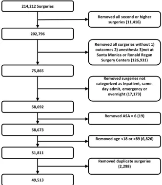
A number of filtering criteria were applied before conducting our analysis, as shown by 57

the CONSORT diagram in Fig 1. If a patient underwent multiple surgeries in a single 58

general anesthesia were considered, as documented by the anesthesiologist note, since 60

we were interested in surgeries with relatively high risk. Any patients that did not have 61

data for the outcome of interest in the database (i.e. had not yet been discharged) were 62

removed from the cohort. Outpatient surgeries were filtered out, and cases with an ASA 63

Physical Status of 6 (organ donors) were also excluded. Patients younger than 18 years 64

old were excluded and anyone older than 89 years old were removed due to 65

HIPAA-based privacy concerns. 66

214,212 Surgeries

Removed all surgeries without 1) outcomes 2) anesthesia 3)not at

Santa Monica or Ronald Regan Surgery Centers (126,931) Removed all second or higher

surgeries (11,416) 202,796

Removed surgeries not categorized as inpatient,

same-day admit, emergency or overnight (17,173)

Removed ASA = 6 (19)

Removed duplicate surgeries (2,298) Removed age <18 or >89 (6,826) 75,865 58,692 58,673 51,811 49,513

Fig 1. Consort DiagramFiltering steps taken to select our cohort.

1.4

Model Input Features

We tested model performance using seven different sets of input features: (1) Charlson 68

comorbidity score [6] as the only input feature, (2) ASA Physical Status as the only 69

input feature, (3) preoperative features without the ASA status, (4) preoperative 70

features and the ASA status, (5) preoperative features with the imputed-ASA score (see 71

Section 1.6), (6) preoperative features and the ASA status, excluding variables 72

indicating how long before surgery each lab is time-stamped as having been run (not 73

ordered), and (7) preoperative features and the imputed-ASA, excluding variables 74

indicating how long before surgery each lab is time-stamped. The lab result time-stamps 75

were removed from feature sets 6 and 7 because, while they may be correlated with 76

negative outcomes, they are not a direct reflection of patient health. All input features, 77

with the exception of the ASA Physical Status, are accessible automatically before 78

surgery via the EMR system (and were extracted here by the PDW). The ASA Physical 79

Status is manually entered into the system by the anesthesiologist after reviewing the 80

patient’s record. Model features include basic patient information such as age, sex, BMI, 81

blood pressure, and pulse, lab tests frequently given prior to surgery such as sodium, 82

potassium, creatinine, and blood cell counts, and surgery specific information such as 83

the surgical codes. In total, 35 preoperative features (including ASA status) were used 84

1.5

Data Preprocessing

Data points greater than 4 standard deviations from the mean were removed. Missing 87

data were imputed using the SoftImpute algorithm [13], as implemented by the 88

fancyimpute Python package [14], with a maximum of 200 iterations. Categorical 89

features were converted into indicator variables, and the first variable was dropped. As 90

the number of positive training examples (in-patient mortalities) was much smaller than 91

the number of negative training examples (survivors), the class balance was greatly 92

skewed (0.61% mortality rate). To overcome this issue, each training set in the 93

cross-validation was oversampled using the SMOTE algorithm [15], implemented in the 94

imblearn Python package [16], using 3 nearest neighbors and the “baseline1” method to 95

create a balanced class distribution. The testing sets were not oversampled and, 96

therefore, maintained the natural outcome frequency. Finally, the training data features 97

were rescaled to have a mean of 0 and standard deviation of 1, and the test data were 98

rescaled using the training data means and standard deviations. 99

1.6

Generating imputed-ASA scores using ASA Status

The ASA Physical Status Classification score is a subjective assessment of a patient’s 101

overall health [17, 18]. The score can take on one of six values, with a score of 1 being a 102

healthy patient and 6 being a brain-dead organ donor [19]. An ASA Physical Status 103

Classification is commonly used in two ways: as a quantitative measure of patient 104

health before a surgery, and for healthcare billing [19]. The ASA Physical Status 105

Classification has been shown to be a useful feature in predicting surgical 106

outcomes [17, 20–22]. However, its inter-rater reliability, a measure of concurrence 107

between scores given by different individuals, is moderate [18]. 108

While the ASA status is a strong predictor of patient health status [17, 20–22], this 109

classification requires a clinician to look through the patient’s chart and subjectively 110

determine the score, which consumes valuable time and requires clinical expertise. In 111

order to balance the value of this score with the desire for automation, we sought to 112

generate a similar metric using readily available data from the EMR - an “imputed” 113

ASA score. Recent works have similarly attempted to develop machine learning 114

approaches to predict ASA scores [23, 24]. However, these methods have difficulty 115

classifying ASA scores of 4 and 5 due to the low frequency of occurrence, and resort to 116

either grouping classes together or ignoring patients with an ASA status of 5. The goal 117

in our work is not to supplant the ASA score but rather to estimate a measure of 118

general patient health for use in our model without needing the time-consuming 119

clinician chart review. 120

Using the existing ASA Physical Status Classification extracted from the EMR data, 121

we trained a gradient boosted tree regression model to predict the ASA status of new 122

patients using preoperative features unrelated to the surgery. The model was 123

implemented using the XGBoost package [25] with 2000 trees and a max tree depth of 7. 124

We used 10-fold cross-validation to generate predictions. This imputed-ASA value is a 125

continuous number, unlike the actual ASA status which is limited to integers. We 126

compared the performance of a model that uses the imputed-ASA scores and 127

preoperative features to a model that uses the actual ASA Physical Status values and 128

preoperative features. 129

1.7

Model Testing and Training

We evaluated four different classification models: logistic regression with two different 131

types of regularization, random forest classifiers, and gradient boosted tree classifiers. 132

ElasticNet [26] penalty, where alpha (regularization constant) and the L1/L2 mixing 134

parameter were set using 5-fold cross-validation. The random forest classifiers were 135

trained with 2000 estimators, Gini impurity as the splitting criterion, and no maximum 136

tree depth was specified. The gradient boosted machine classifiers were trained using 137

2000 estimators and a max tree depth of 5. All predictions were made using 10-fold 138

cross-validation on the entire dataset. The logistic regression and random forest 139

classifiers were implemented using Scikit-learn [27], and the gradient boosted tree 140

classifiers were implemented using the XGBoost package [25]. All performance metrics 141

were calculated using methods implemented by Scikit-learn [27]. 142

1.8

Feature Importance

To determine which features were most important to the classification models, we 144

examined the model weights for linear models, the feature (Gini) importance for the 145

random forest models, and the feature weight (number of times a feature appears in a 146

tree) for the gradient boosted tree models. 147

1.9

Integrating Preoperative Risk with Postoperative Risk

Previous work [11] has shown that integrating a measure of preoperative risk into a 149

postoperative mortality risk prediction model increases the model performance. We 150

integrated the risk predictions of our random forest model with the previously 151

developed postoperative model in order to see if our model predictions can similarly 152

serve this function. Using the deep neural network architecture and features used by 153

Lee et al. [11], we replaced the ASA status feature with the preoperative risk score 154

(generated using the random forest model with preoperative features and imputed-ASA 155

scores) and trained the model on the same cohort used for preoperative risk prediction. 156

The intraoperative data were preprocessed in the same manner as described in [11]. We 157

then compared the area under the ROC of the postoperative model trained using the 158

ASA status and intraoperative features to the postoperative model that was trained 159

using the preoperative risk score and intraoperative features. 160

1.10

Generating Charlson Comorbidity Indexes

We compared our method with the Charlson Comorbidity Index scores [6], a well-known 162

and proven existing method for prediction of risk of postoperative mortality, for each 163

patient in the cohort. We used the updated weights as described by Quan et al. [28]. 164

Scores were calculated using the R packageicd [29] on all ICD10 codes associated with 165

each surgery admission. 166

2

Results

2.1

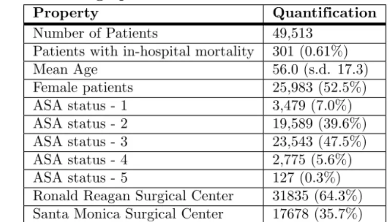
Patient Demographics

The patient dataset contained 49,513 surgical records (see Table 1). These patients were 169

between the ages of 18 and 89, with a mean age of 56, and were treated as either 170

inpatients, same-day admits, emergencies, or overnight recoveries. The frequency of 171

mortality in the dataset was approximately 0.61%. A patient ASA status of 3 was the 172

Table 1. Patient Demographics

Property Quantification

Number of Patients 49,513

Patients with in-hospital mortality 301 (0.61%)

Mean Age 56.0 (s.d. 17.3) Female patients 25,983 (52.5%) ASA status - 1 3,479 (7.0%) ASA status - 2 19,589 (39.6%) ASA status - 3 23,543 (47.5%) ASA status - 4 2,775 (5.6%) ASA status - 5 127 (0.3%)

Ronald Reagan Surgical Center 31835 (64.3%)

Santa Monica Surgical Center 17678 (35.7%)

Patient demographics for the cohort used for training and testing models. Number of patients and percent of the total cohort are shown.

2.2

Model Performance

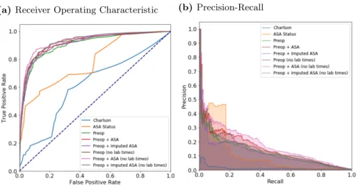
2.2.1 Area under the receiver operating characteristic (ROC) curve 175

The area under the ROC curve values for each model are shown in Table 2 and ROC 176

curves are shown for the random forest model in Fig 2a and for all models in 177

Supplemental Fig S1. Models using the preoperative features have higher area under 178

the ROC values (0.909, 95%CI 0.881-0.937) than the models that use either the 179

Charlson comorbidity score (0.706, 95%CI 0.669-0.744) or the ASA status (0.865, 180

95%CI 0.848-0.882). Adding the imputed-ASA status values to the preoperative 181

features improves the area under the ROC (0.912, 95%CI 0.902-0.923), but using the 182

true ASA value assigned by anesthesiologists, along with the preoperative features, 183

produces the highest area under the ROC value (0.920, 95%CI 0.907-0.932), although 184

the difference is not statistically significant as compared with the imputed value. 185

Reducing the preoperative feature set by removing variables indicating when the lab 186

tests were administered before surgery further increases the area under the ROC of both 187

the preoperative features and imputed-ASA (0.921, 95%CI 0.908-0.934) and the 188

preoperative features and true ASA status (0.929, 95%CI 0.915-0.943). The Random 189

Forest model has the best performance of all models used (see Table 2). 190

2.2.2 Calibration 191

A well-calibrated binary classification model outputs probabilities that are close to the 192

true label (either a 1 for positive examples, or 0 for negative examples). Model 193

calibration is often measured using the Brier score, which is the average squared 194

distance between the predicted probability of the outcome and the true label over all 195

samples. We used this metric to assess the calibration of our models, as shown in 196

Table 3. The non-linear models (Random Forest, XGBoost) had much lower Brier 197

scores compared to the linear models (Logistic Regression, ElasticNet). When using 198

either the Charlson comorbidity score or the ASA status as the only feature, the 199

XGBoost classifier had the lowest Brier score (0.0468 and 0.0486, respectively). For the 200

the other five feature sets the random forest models obtained the lowest Brier scores 201

(a)Receiver Operating Characteristic (b) Precision-Recall

Fig 2. Receiver operating characteristic (ROC) and precision recall curves for the random forest modelPlots were generated using 10-fold cross-validated predictions on the entire dataset. ROC curves (a) show the false positive rate on the x-axis and the true positive rate on the y-axis. The optimal point is the upper-left corner. Precision-recall curves (b) show the recall on the x-axis and precision on the y-axis. The optimal point is in the upper-right corner.

Table 2. Mortality Prediction Performance using AUROC curve Model / AUC (95% CI) Logistic Regression ElasticNet Classifier Random Forest XGBoost Classifier Charlson Comorbidity 0.706 (0.669-0.744) 0.706 (0.669-0.744) 0.692 (0.655-0.728) 0.692 (0.655-0.728) ASA Status 0.865 (0.848-0.882) 0.865 (0.848-0.882) 0.828 (0.766-0.890) 0.828 (0.766-0.890) Preop Features 0.872 (0.840-0.903) 0.888 (0.860-0.917) 0.909 (0.881-0.937) 0.895 (0.863-0.927) Preop + ASA Status 0.883 (0.855-0.910) 0.905 (0.883-0.928) 0.920 (0.907-0.932) 0.919 (0.904-0.934) Preop + imputed-ASA 0.868 (0.841-0.895) 0.890 (0.868-0.912) 0.912 (0.902-0.923) 0.901 (0.884-0.917) Preop (No Time)

+ ASA Status 0.886 (0.859-0.914) 0.908 (0.883-0.932) 0.929 (0.915-0.943) 0.916 (0.904-0.927) Preop (No Time)

+ imputed-ASA 0.871 (0.841-0.900) 0.891 (0.868-0.914) 0.921 (0.908-0.934) 0.897 (0.881-0.912) Area under the ROC (AUROC) curve values for each model and each of the seven input feature sets, using 10-fold cross-validation. Models with the highest AUROC are shown in bold. The mean value of the AUROC is shown, along with the 95% confidence interval (¯x±1.96×σ/√n) in parenthesis. When using either the Charlson comorbidity or the ASA status as the only input feature, the linear models (Logistic regression, ElasticNet) outperform the non-linear models (Random Forest, XGBoost). However, for feature sets using more than one feature, the non-linear models outperform the linear models. In particular, the Random Forest has the highest AUROC compared to the other models.

2.2.3 Precision-Recall 203

While the ROC curves are very informative of binary classification prediction 204

performance in general, the precision-recall curves can be more informative when the 205

classes are highly imbalanced [30]. However, these plots are often not included in 206

methods for predicting surgical mortality, in which the datasets are inherently 207

imbalanced. 208

An optimal model would reach the point in the upper-right corner of the PR plot 209

(i.e. perfect recall and perfect precision). Using the random forest model, PR curves for 210

each of the sets of features are shown in Figs 2b and, for all models, in Fig S2. As 211

poor precision-recall. Including the ASA status as an input feature increases the 213

precision-recall compared to only using the preoperative features alone. The feature set 214

using only the ASA status does surprisingly well, likely due to individuals with an ASA 215

score of 5 being highly enriched for mortality and the difficulty of imputing ASA scores. 216

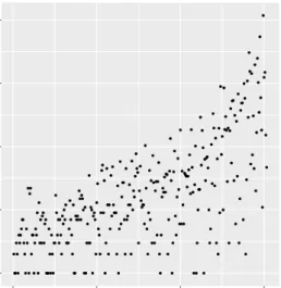
A clinically-relevant question to ask is how many additional patients must be flagged 217

to capture one additional mortality; this is an extension of the “number needed to treat” 218

idea for a risk ordered population. In Fig 3, the marginal increase in the number needed 219

to be flagged is plotted as a function of the number of mortalities captured, using the 220

risk scores generated from the random forest model. For the first hundred mortalities, 221

this number ranges between one and ten with limited exceptions. After the first 222

hundred mortalities however, the marginal increase is often in the hundreds and 223

sometimes thousands of additional patients. 224

● ●● ● ● ● ● ● ● ● ●● ● ● ● ● ● ● ● ● ● ● ● ● ● ● ● ● ● ● ● ● ● ● ●● ● ●● ● ●● ● ● ● ● ● ● ● ● ● ● ● ● ● ● ● ● ● ● ● ● ● ●●● ● ● ● ● ● ● ●● ● ● ● ● ● ● ● ● ● ● ● ● ● ● ● ● ● ● ● ● ● ●● ● ● ● ● ● ● ● ● ● ● ● ● ● ● ● ● ● ● ● ● ● ● ● ●●● ● ● ● ● ● ● ● ●● ● ● ● ● ● ● ● ● ● ● ● ● ● ● ● ● ● ● ● ● ● ●●● ● ● ● ● ● ● ● ● ● ● ● ● ● ● ● ● ● ● ● ● ● ● ● ● ● ● ●● ● ● ● ● ● ● ● ● ● ● ● ● ● ● ● ● ● ● ● ● ●● ● ● ● ● ● ● ● ● ● ● ● ● ● ● ● ●● ● ● ● ● ● ● ● ●● ● ● ● ● ● ● ● ● ● ● ● ● ● ● ● ● ● ● ● ● ● ● ● ● ● ● ● ● ● ● ● ● ● ● ● ● ● ● ● ● ●● ● ● ● ● ● ● ● ● ● ● ● ● ● ● ● ● ● ● ● ● ● ● ● ● ● ● ● ● ● 100 101 102 103 104 0 100 200 300 Deaths Marginal Increase In P atients

Fig 3. Marginal increase in number of patients needed to capture one additional deathThis figure shows the marginal increase in the number of patients that need to be treated as a function of the number of in-hospital mortalities that will be captured. Note that the marginal increase in number of patients is log-scaled.

2.3

Feature Importance

To determine the most important features for each of the models, we examined the 226

feature weights of the linear models and feature importances of the non-linear models. 227

The top five most important features of each model, when trained on the preoperative 228

features excluding the time to surgery of laboratory tests, are shown in Table 6. For the 229

feature importance using other combinations of ASA and time to surgery of laboratory 230

tests, see Tables S10, S11 and S12. As expected [20–22, 31], the ASA status is the most 231

important feature of every model where it is contained. Interestingly, there were as 232

many important features shared by the ElasticNet model and the XGBoost model as 233

there were by the random forest and the XGBoost model (as shown by the bold 234

numbers in Table 6). Notably, the random forest model placed more importance on 235

surgery-specific information, like patient class and pre-surgery location, whereas the 236

XGBoost model placed higher importance on the lab results. 237

In Table 7, the feature importance for the random forest model is shown using four 238

different sets of input features. For the feature sets that include lab result timestamps, 239

when these features are removed, the feature importance shifts to the lab results 241

themselves, as well as surgery-specific features such as the patient class. 242

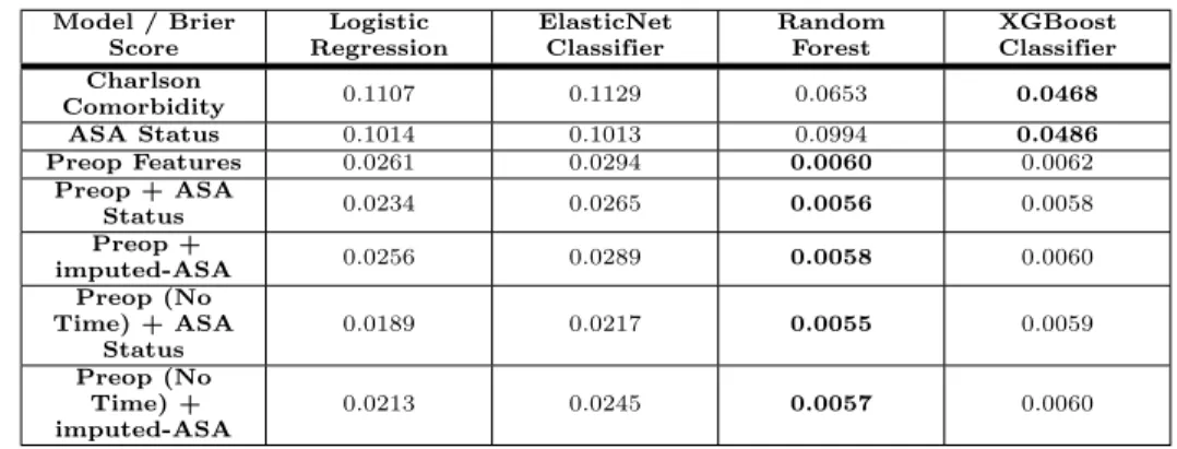
Table 3. Calibration of Models: Brier Score Model / Brier Score Logistic Regression ElasticNet Classifier Random Forest XGBoost Classifier Charlson Comorbidity 0.1107 0.1129 0.0653 0.0468 ASA Status 0.1014 0.1013 0.0994 0.0486 Preop Features 0.0261 0.0294 0.0060 0.0062 Preop + ASA Status 0.0234 0.0265 0.0056 0.0058 Preop + imputed-ASA 0.0256 0.0289 0.0058 0.0060 Preop (No Time) + ASA Status 0.0189 0.0217 0.0055 0.0059 Preop (No Time) + imputed-ASA 0.0213 0.0245 0.0057 0.0060

Calibration of the models was measured using the Brier score (lower is better). Models with the lowest Brier score are shown in bold. The non-linear classifiers (Random Forest, XGBoost) consistently have lower Brier scores compared to the linear classifiers (Logistic Regression, ElasticNet).

2.4

Integrating Preoperative Risk with Postoperative Risk

Replacing the ASA status with the preoperative risk predictions in the postoperative 244

risk prediction model generated similar results. The postoperative risk model that was 245

trained using the preoperative risk scores had an area under the ROC of 0.924 (95%CI 246

0.905-0.941), whereas the postoperative model trained using the ASA status had an 247

area under the ROC of 0.929 (95%CI 0.911-0.944). This is in line with the previously 248

published results of this model [11]. Interestingly, the area under the ROC of the 249

preoperative model is similar to the area under the ROC of the postoperative model, 250

which suggests that the postoperative features may not be capturing additional 251

information. 252

In order to examine how mortality risk changes from immediately before surgery to 253

after surgery, the preoperative and postoperative risk scores for all patients were 254

grouped by percentiles and the counts of each grouping are displayed in Table 4 and 255

with a heatmap (Fig 4a). For the majority of patients we see a slight increase or 256

decrease in their postoperative risk compared to the initial preoperative risk, as 257

demonstrated by the coloring just above/below the diagonal line in Fig 4a. Fig 4b 258

demonstrates the same plot, but contains only those patients who eventually died 259

during that admission, and the corresponding data can be found in Table 5. Note that 260

most of these patients fall in the upper right quadrant high-risk quadrant of the 261

heatmap (Fig 4b). Moreover, 78% of patients who die and have a preoperative risk 262

percentile below 95% have an increased postoperative risk percentile. This is 263

substantially greater than the percent of matched patients from a null distribution who 264

have an increased percentile (see Fig S5). 265

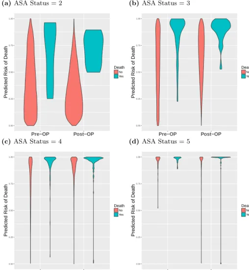
The change in risk between the preoperative and postoperative time points is shown 266

using violin plots in Fig 5, where the risk scores are binned by percentile and stratified 267

by ASA status. In all four subplots of Fig 5, the in-hospital mortalities are, on average, 268

at higher risk than the patients who survive surgery, as shown by the increased mass 269

toward the top of the blue plots compared to the red plots. This is particularly 270

apparent in Figs 5a and 5b as the majority of patients have an ASA status of 2 and 3, 271

and therefore the violins are larger. In Figs 5c and 5d, most of the patients begin and 272

we can see that the models correctly rank those that die at higher risk, as shown by the 274

increased mass toward the top of the blue plots compared to the red. Violin plots for 275

patients with an ASA status of 1 are not shown as none of those patients died during 276

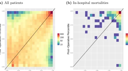
(a)All patients 0.00 0.25 0.50 0.75 1.00 0.00 0.25 0.50 0.75 1.00 Pre−Operative Percentile P ost−Oper ativ e P ercentile 10 50 200 800 (b) In-hospital mortalities 0.00 0.25 0.50 0.75 1.00 0.25 0.50 0.75 1.00 Pre−Operative Percentile P ost−Oper ativ e P ercentile 5 20 100

Fig 4. Heatmap of Preoperative Risk vs. Postoperative RiskPreoperative (x-axis) and postoperative (y-axis) risk scores were binned by percentile, and the counts

per bin visualized as a heatmap in log scale. Preoperative risk predictions were generated using the random forest model trained on the preoperative features, including lab times, and the imputed-ASA status. In (a) all patients are displayed, and in (b) only the in-hospital mortalities are shown. 78% of patients who die and have a

pre-operative risk percentile below 95% have an increased postoperative risk percentile. This is substantially greater than the percent of matched patients from a null

distribution who have an increased percentile, see Fig S5.

3

Discussion

In this manuscript we were able to successfully create a fully-automated preoperative 279

risk prediction score that can better predict in-hospital mortality than both the ASA 280

Score and the Charlson comorbidity index. Unlike the ASA status or the Charlson 281

comorbidity scores, this score was built using solely objective clinical information that 282

was readily available from the EMR prior to surgery. Similar to previous models [11], 283

the results indicate that inclusion of the ASA score in the model improves the predictive 284

ability. However, we were able to account for this by “imputing” the ASA score and 285

including this additional feature in our model. We were additionally able to integrate 286

the results of our model into a previously developed postoperative risk prediction model 287

and achieve a performance that was comparable to the use of the ASA physical status 288

score in that model. Lastly, when using the preoperative and postoperative scores 289

together we were able to demonstrate that, on a patient level, risk does change during 290

the perioperative period - indicating that choices made in the operating room may have 291

profound implications for our patients. 292

The challenge of perioperative risk stratification is certainly not new. In fact, the 293

presence of so many varied risk scores (ASA Score, Charlson Comorbidity Index [6], 294

POSPOM [4], RQI [32], NSQIP Risk Calculator [8]) speaks to the importance with 295

which clinicians view this problem. A major limitation of many of these models has 296

been that they either rely on data not available at the time of surgery (i.e. ICD codes), 297

or they require an anesthesiologist to review the chart (those that contain the ASA 298

score). The fact that our model can be fully automated and yet perform better than 299

these models implies that it has broad applicability. 300

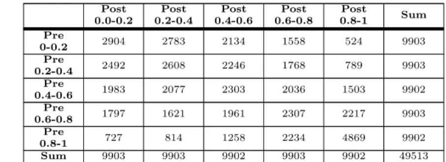
Table 4. Flow of from Pre- to Post-operative Percentile Bins Post 0.0-0.2 Post 0.2-0.4 Post 0.4-0.6 Post 0.6-0.8 Post 0.8-1 Sum Pre 0-0.2 2904 2783 2134 1558 524 9903 Pre 0.2-0.4 2492 2608 2246 1768 789 9903 Pre 0.4-0.6 1983 2077 2303 2036 1503 9902 Pre 0.6-0.8 1797 1621 1961 2307 2217 9903 Pre 0.8-1 727 814 1258 2234 4869 9902 Sum 9903 9903 9902 9903 9902 49513

This tables shows how the number of patients in each risk percentile bin change between before and after surgery. Bins are defined by the percentile of a patient’s risk score relative to all other patients.

Table 5. Change in Pre- to Post-operative Risk Percentile Bins for In-hospital Mortalities Post 0.0-0.2 Post 0.2-0.4 Post 0.4-0.6 Post 0.6-0.8 Post 0.8-1.0 Sum Pre 0-0.2 0 0 0 0 1 1 Pre 0.2-0.4 0 0 0 3 5 8 Pre 0.4-0.6 0 0 1 4 6 11 Pre 0.6-0.8 0 0 1 0 20 21 Pre 0.8-1 4 0 5 9 244 262 Sum 4 0 7 16 276 303

This tables shows how the number of in-hospital mortalities in each risk percentile bin change between before and after surgery. There is an increase in the number of postoperative high-risk patients (0.8-1.0) compared to preoperative high-risk patients (0.8-1.0).

good predictor of postoperative outcomes. We believe that one reason that our model is 302

able to outperform the ASA score is related to the overwhelming amount of information 303

contained in the modern patient’s medical record. The introduction of the EMR has 304

lead to an explosion of information that can frequently make it challenging for a 305

clinician to consume everything. For example, due to time constraints, an 306

anesthesiologist may not be able to fully assess the impact of every entry in a patient’s 307

health record before an upcoming procedure. This limitation of a clinician’s ability to 308

find all of the relevant information in the modern EMR highlights the advantage of an 309

automated scoring system such as this - not as a replacement for physicians - but rather 310

as a tool to help them better focus their efforts on those patients most likely to benefit. 311

Our efforts to leverage the value of the ASA score led us to create an “imputed” 312

ASA score for us to include in our model. However, the creation and inclusion of this 313

feature did not significantly improve the predictive power of our model. It is important 314

to note that this is not truly an imputation of, or replacement to, the ASA score. Our 315

techniques and the ASA score differ in some key respects. First, while the ASA score is 316

an ordinal score with values between 1 and 5, our score is actually a continuous variable 317

with no such thresholds. Second, the ASA score itself is not designed to predict 318

practicing clinicians to categorize their patients. We believe that the fact that the ASA 320

score is not designed to predict any specific postoperative outcome is a potential 321

advantage of using these analytic techniques. While the model that is presented here 322

was optimized to focus on postoperative mortality, the same techniques could easily be 323

used to help predict a wide range of postoperative outcomes such as acute kidney injury, 324

respiratory failure, readmission and others. Such a refined classification would not be 325

possible with the ASA or any other generalizable risk score. 326

Another advantage of an automated model such as this is that it allows for the 327

continuous recalculation of risk longitudinally over time. As shown in Fig 4, most 328

patients have either a minor increase or decrease in risk in the time from before to after 329

surgery and, unsurprisingly, in patients who eventually die, that risk tends to increase. 330

We believe that this finding has several important implications. First, given the 331

challenges of continually monitoring the risk of all patients in the hospital, advanced 332

analytical models such as the models proposed in this manuscript have great potential 333

to act as early warning systems alerting clinicians to sudden changes in risk profiles and 334

facilitating the use of rapid response teams. Second, the frequency with which risk 335

changed substantially during the operative period highlights the effect to which 336

intraoperative interventions may have implications far beyond the operating room. 337

Multiple specific interventions, including the avoidance of intraoperative hypotension 338

and hypothermia, have been shown to have effects on longer-term outcomes, and 339

currently enhanced recovery after surgery (ERAS) pathways have promoted the 340

standardization of intraoperative interventions. We believe that our findings should add 341

to the evidence that a well-prescribed anesthetic plan may be of longer-term benefit to 342

patient outcomes. 343

One potential promise of the use of machine learning in medicine is the ability to 344

leverage these models in order to better understand what features are truly driving 345

outcomes. In an effort to better understand this, we extracted the weights of the 346

features in both the linear and non-linear models. Of note, removing some features, 347

specifically the relative time of lab tests, actually improved the results of our model. 348

This could potentially be caused by multiple correlated features tagging an underlying 349

cause, and the correlation introduces noise in the model as the importance is distributed 350

among multiple features rather than focused on a single feature. In theory, a machine 351

learning model should be able to remove these features by setting a coefficient to zero. 352

However, in practice, this may not always be the case - as illustrated here, where we 353

force this behavior by manually removing the features from the model. We believe that 354

this finding highlights the importance of having collaborative relationships between 355

experts in machine learning and clinicians who are able to help guide which features to 356

include in a model. Simply entering large amounts of data from an EMR, without 357

proper clinical context, is unlikely to create the most effective or efficient models. 358

There are several key limitations of this study. Perhaps the most significant is the 359

low frequency of the outcome in question - in-hospital mortality. The incidence of 360

mortality was less than 1% - implying that a model that blindly reports “survives” 361

every time will have an accuracy greater than 99%. Predicting such a rare outcome 362

makes it highly challenging to produce results with very high precision. Nonetheless, 363

the models presented in this paper do outperform other models currently in use, as 364

measured by area under the ROC curve. Secondly, the data used here are from a single 365

large academic medical center. Thus, it is possible, though unlikely, that this model will 366

not perform similarly at another institution. Past experience has demonstrated that, 367

with recalibration, models can easily be transported from one institution to another. 368

One last limitation lies not necessarily with the study itself but rather with the overall 369

landscape of EMR data. While the promises of fully-automated risk scores are great, 370

the EMRs. Thus, in order to truly automate processes such as these, robust data 372

interoperability standards (such as Fast Healthcare Interoperability Resources (FHIR)) 373

will be needed in order to allow access to data. 374

4

Conclusion

The promise of using machine learning techniques in healthcare is great. In this work 376

we have presented a novel set of easily-accessible (via EMR data) preoperative features 377

that are combined in a machine learning model for predicting in-hospital post-surgical 378

mortality, which outperforms current clinical risk scores. We have also shown that the 379

risk of in-hospital mortality changes over time, and that monitoring that risk at 380

multiple time-points will allow clinicians to make better data-driven decisions and 381

provide better patient care. It is our hope and expectation that the next few years will 382

produce a plethora of research leveraging data obtained during routine patient care to 383

improve care delivery models and outcomes for all of our patients. 384

Table 6. Model Feature Importance: Without ASA and Without Lab Time Features

Feature Random

Forest

Linear

Regression Elastic Net XGBoost

ALBUMIN 0.04* -0.57 -0.48 0.03* BNP 0.04* 1.45* 1.12* 0.03* HEMOGLOBIN 0.05* -0.8 -0.77 0.03* INR 0.05* 1.14 0.76 0.02 PAT CLASS INPATIENT 0.06* -0.67 -0.12 0.02

PAT CLASS SAME

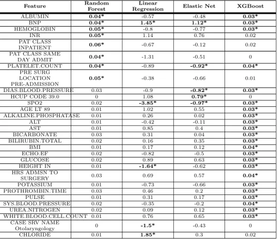
DAY ADMIT 0.04* -1.31 -0.51 0 PLATELET.COUNT 0.04* -0.89 -0.92* 0.04* PRE SURG LOCATION PRE-ADMISSION 0.05* -0.38 -0.66 0.01 DIAS.BLOOD.PRESSURE 0.03 -0.9 -0.82* 0.03* HCUP CODE 39.0 0 1.08 0.79* 0 SPO2 0.02 -3.85* -0.97* 0.03* AGE LT 89 0.01 1.02 0.55 0.03* ALKALINE.PHOSPHATASE 0.01 0.26 0.02 0.03* ALT 0.01 -0.42 -0.11 0.03* AST 0.01 0.85 0.4 0.03* BICARBONATE 0.03 0.31 0.04 0.03* BILIRUBIN.TOTAL 0.02 0.16 0.35 0.03* BMI 0.01 0.17 0.12 0.04* ECHO.EF 0.02 -0.82 -0.5 0.03* GLUCOSE 0.02 0.89 0.63 0.03* HEIGHT IN 0.01 -1.64* -0.62 0.03* HRS ADMSN TO SURGERY 0.03 0.69 0.57 0.04* POTASSIUM 0.01 -0.73 -0.66 0.03* PROTHROMBIN.TIME 0.03 0.46 0.2 0.03* PULSE 0.01 0.31 0.17 0.03* SYS.BLOOD.PRESSURE 0.02 -0.35 -0.2 0.04* UREA.NITROGEN 0.02 0.09 0.12 0.03* WHITE.BLOOD.CELL.COUNT 0.01 0.76 0.65 0.03* CASE SRV NAME Otolaryngology 0 -1.5* -0.43 0 CHLORIDE 0.01 1.85* 0.3 0.02

The bold values with the * indicates that the value was one of the top five strongest predictors for the given model. In the Logistic Regression and ElasticNet columns the model weights are shown, where negative values indicate the feature lowers the probability of mortality. The non-linear model features are ranked according to the mean decrease in Gini impurity.

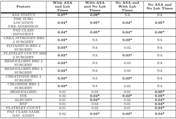
Table 7. Random Forest Feature Importance Feature With ASA and Lab Times With ASA and No Lab Times No ASA and With Lab Times No ASA and No Lab Times ASA STATUS 0.07* 0.08* NA NA PRE SURG LOCATION PRE-ADMISSION 0.04* 0.05* 0.04* 0.05* PAT CLASS INPATIENT 0.04* 0.05* 0.04* 0.06* UREA.NITROGEN.HRS 2 SURGERY 0.03* NA 0.03* NA POTASSIUM.HRS 2 SURGERY 0.03* NA 0.02 NA PLATELET.COUNT.HRS 2 SURGERY 0.03* NA 0.03* NA HEMOGLOBIN.HRS 2 SURGERY 0.03* NA 0.02 NA HEMOGLOBIN.HRS 2 SURGERY 0.03* NA 0.02 NA CREATININE.HRS 2 SURGERY 0.03* NA 0.03* NA CHLORIDE.HRS 2 SURGERY 0.03* NA 0.02 NA HEMOGLOBIN 0.01 0.03 0.01 0.05* INR 0.02 0.04* 0.03* 0.05* ALBUMIN 0.01 0.04* 0.02 0.04* BNP 0.01 0.03 0.01 0.04* PLATELET.COUNT 0.01 0.03 0.01 0.04*

PAT CLASS SAME

DAY ADMIT 0.02 0.04* 0.03* 0.04*

The top five features of the random forest model, ranked by Gini importance, for each feature set are shown in bold and have an asterisk. Features with a NA value were not included in the dataset. All models included the preoperative features. “No ASA” means the ASA status was not included as a feature, and “No Lab Times” means the timestamps of the lab results were not included (i.e. features with the “.HRS 2 SURGERY” suffix).

(a)ASA Status = 2 0.00 0.25 0.50 0.75 1.00 Pre−OP Post−OP

Predicted Risk of Death

Death No Yes (b) ASA Status = 3 0.00 0.25 0.50 0.75 1.00 Pre−OP Post−OP

Predicted Risk of Death

Death No Yes (c) ASA Status = 4 0.00 0.25 0.50 0.75 1.00 Pre−OP Post−OP

Predicted Risk of Death

Death No Yes (d) ASA Status = 5 0.00 0.25 0.50 0.75 1.00 Pre−OP Post−OP

Predicted Risk of Death

Death

No Yes

Fig 5. Comparison of preoperative and postoperative mortality predictions binned by percentileViolin plots showing the percentile rankings of the mortality risk prediction scores relative to all other individuals, stratified by ASA status. Preoperative risk (2 left violins of each plot) and postoperative risk (right 2 violins of each plot) are shown in each plot. Red violins are patients that survived surgery, and blue violins are mortalities.

Supporting Information

Fig S1. Receiver Operating Characteristic (ROC) curvesROC curves show the false positive rate on the x-axis and the true positive rate on the y-axis. The optimal point is the upper-left corner. Plots were generated using cross-validated predictions on entire dataset. Models that use preoperative features consistently outperform models that only use Charlson score or ASA status. Logistic Regression (a) and ElasticNet (b) (linear models) outperform Random Forest (c) and XGBoost (d) (non-linear models) when using a single input feature. However, non-linear models (c, d)

outperform linear models (a, b) when using multiple features.

Fig S2. Precision-recall (PR) curvesPR curves show the recall on the x-axis and precision on the y-axis. The optimal point is in the upper-right corner. Figs (a) and (b) show that the linear models have very similar PR curves. The gradient boosted trees model (d) has better precision-recall compared to the random forest (c).

Fig S3. Change in preoperative and postoperative mortality prediction rankPoints on the left of the plot are preoperative predictions of mortality, and points on the right are postoperative predictions of mortality. The preoperative probability predictions were ranked from highest to lowest, and for each patient a line from the preoperative prediction is then connected to the rank in list of sorted postop predictions. If a point does not change its rank in the list of risk scores, then the line will be straight across. Otherwise if the rank increased, it will have positive slope, or negative slope if it decreased. Blue lines are patients that survived surgery, and red lines are in-hospital mortalities. The median survivor points are displayed by the yellow line. Spearman rank-order correlation coefficient and p-value are shown above each plot.

Fig S4. Comparison of preoperative and postoperative mortality prediction using risk scoresViolin plots showing the distributions of mortality risk, stratified by ASA status. Preoperative risk (2 left violins of each plot) and postoperative risk (right 2 violins of each plot) are shown in each plot. Red violins are patients that died during surgery, and blue violins are survivors.

Fig S5. Null distribution of increasing risk for matched individuals based on similar pre-operative scoresFor each individual who died, we found a matched individual who falls within one percentile of the pre-operative risk percentile of the individual that died. We then calculated the number of individuals in this matched set who had increased chance of death for their post-operative score. We repeated this process 10,000 times. This histogram represents the percent of matched individuals that have a higher post-operative score than pre-operative score. We restrict our analysis to individuals who fall in less than the ninety-fifth percentile.

Table S1. Feature List Preoperative features used in the model. All features are readily available via the EHR system prior to surgery. HCUP codes are included as features, but not shown in this table. Refer to Table S2 for a full list of HCUP codes.

Table S2. Comparison of HCUP codes between overall surgeries and surgeries with deathThe numbers in parentheses () in the Count and Percent columns represent the count and percentage of individuals who died in-hospital undergoing surgery who were classified under the given HCUP description. Table S3. Predicting Mortality using Preoperative FeaturesModel

performance metrics for predicting mortality using preoperative features and 10-fold cross-validation.

True positives: TP, False positives: FP, True negatives: TN, False negatives: FN. Accuracy = (TP+TN)/(TP+TN+FP+FN). Precision = TP/(TP+FP).

Recall = TP/(TP+FN).

Specificity = TN/(TN+FP). F1 Score = 2/((1/Recall)+(1/Precision)).

Table S4. Predicting Mortality using Preoperative Features + ASA Status Model performance metrics for predicting mortality using both preoperative features and ASA status as input features, and 10-fold cross-validation. For an explanation of the metrics see the description of Table S3

Table S5. Predicting Mortality using ASA StatusModel performance metrics for predicting mortality using only the ASA status as an input feature, and 10-fold cross-validation. For an explanation of the metrics see the description of Table S3 Table S6. Predicting Mortality using Charlson ComorbidityModel

performance metrics for predicting mortality using only the Charlson comorbidity as an input feature, and 10-fold cross-validation. For an explanation of the metrics see the description of Table S3

Table S7. Predicting Mortality using Preoperative Features +

imputed-ASA ScoreModel performance metrics for predicting mortality using both preoperative features and the imputed-ASA score as input features, and 10-fold cross-validation. For an explanation of the metrics see the description of Table S3 Table S8. Predicting Mortality using Preoperative Features + ASA status, Without Lab TimesModel performance metrics for predicting mortality using both preoperative features and the ASA score but without lab times as input features, and 10-fold cross-validation. For an explanation of the metrics see the description of Table S3 Table S9. Predicting Mortality using Preoperative Features +

imputed-ASA status, Without Lab TimesModel performance metrics for predicting mortality using both preoperative features and the imputed-ASA score but without lab times as input features, and 10-fold cross-validation. For an explanation of the metrics see the description of Table S3

Table S10. Model Feature Importance: With ASA and Without Lab Time FeaturesThe bold values with the * indicates that the value was one of the top five strongest predictors for the given model. In the Logistic Regression and ElasticNet columns the model weights are shown, where negative values indicate the feature lowers the probability of mortality. The non-linear model features are ranked according to the mean decrease in Gini impurity.

Table S11. Model Feature Importance: Without ASA and With Lab Time FeaturesThe bold values with the * indicates that the value was one of the top five strongest predictors for the given model. In the Logistic Regression and ElasticNet columns the model weights are shown, where negative values indicate the feature lowers the probability of mortality. The non-linear model features are ranked according to the mean decrease in Gini impurity.

Table S12. Model Feature Importance: With ASA and Time FeaturesThe bold values with the * indicates that the value was one of the top five strongest predictors for the given model. In the Logistic Regression and ElasticNet columns the model weights are shown, where negative values indicate the feature lowers the probability of mortality. The non-linear model features are ranked according to the mean decrease in Gini impurity.

Table S13. Change in Pre- to Post-operative Risk using ASA-like risk bins This tables shows how risk changes for groups defined by the number of patients with each ASA score, from 1 to 5. Patient risk scores were sorted from highest-risk to lowest risk, and then patients were binned into 5 categories, where the number of patients in each category corresponds to the number of patients in each ASA status group. For example, 127 patients had an ASA status of 5, therefore, bins Pre 5 and Post 5 each have 127 patients.

Table S14. Change in Pre- to Post-operative Risk using ASA-like risk bins for In-hospital MortalitiesThis tables shows how risk changes for groups defined by the number of patients with each ASA score, from 1 to 5. Patient risk scores were sorted from highest-risk to lowest risk, and then patients were binned into 5 categories, where the number of patients in each category corresponds to the number of patients in each ASA status group. In this table we only show in-hospital mortalities. The number of patients in group 5 increases between the preoperative and postoperative periods, showing that the postoperative model is capturing the increased risk derived from intraoperative data.

Acknowledgments

L.O.L. was financially supported by the National Institute of Mental Health under 387

award number K99MH116115. S.S. was supported in part by NIH grants R00GM111744, 388

R35GM125055, NSF Grant III-1705121, an Alfred P. Sloan Research Fellowship, and a 389

gift from the Okawa Foundation. R.B. was funded by a UCLA QCB Collaboratory 390

Postdoctoral Fellowship directed by Matteo Pellegrini. U.M. was financially supported 391

by the Bial Foundation. B.J. was supported by the National Science Foundation 392

Graduate Research Fellowship Program under Grant No. DGE-1650604. 393

M.C. is co-owner of US patent serial no. 61/432,081 for a closed-loop fluid 394

administration system based on the dynamic predictors of fluid responsiveness which 395

has been licensed to Edwards Lifesciences. M.C. is a consultant for Edwards 396

Lifesciences (Irvine, CA), Medtronic (Boulder, CO), Masimo Corp. (Irvine, CA). M.C. 397

has received research support from Edwards Lifesciences through his Department and 398

NIH R01 GM117622 - Machine learning of physiological variables to predict diagnose 399

and treat cardiorespiratory instability and NIH R01 NR013912 - Predicting Patient 400

Instability Non invasively for Nursing Care-Two (PPINNC-2). No funding bodies had 401

any role in study design, data collection and analysis, decision to publish, or 402

References

1. Pearse RM, Harrison DA, James P, Watson D, Hinds C, Rhodes A, et al. Identification and characterisation of the high-risk surgical population in the United Kingdom. Critical Care. 2006;10(3):R81. doi:10.1186/cc4928.

2. Kang DH, Kim YJ, Kim SH, Sun BJ, Kim DH, Yun SC, et al. Early surgery versus conventional treatment for infective endocarditis. New England Journal of Medicine. 2012;366(26):2466–2473.

3. Leeds IL, Truta B, Parian AM, Chen SY, Efron JE, Gearhart SL, et al. Early Surgical Intervention for Acute Ulcerative Colitis Is Associated with Improved Postoperative Outcomes. Journal of Gastrointestinal Surgery.

2017;21(10):1675–1682.

4. Le Manach Y, Collins G, Rodseth R, Le Bihan-Benjamin C, Biccard B, Riou B, et al. Preoperative Score to Predict Postoperative Mortality (POSPOM) Derivation and Validation. Anesthesiology: The Journal of the American Society of Anesthesiologists. 2016;124(3):570–579.

5. Sessler Daniel I MD, Sigl Jeffrey C PD, Manberg Paul J PD, Kelley Scott D MD, Schubert M B A , Armin MD, Chamoun Nassib G MS. Broadly Applicable Risk Stratification System for Predicting Duration of Hospitalization and Mortality. Anesthesiology. 2010;113(5):1026–1037.

6. Charlson M, Szatrowski TP, Peterson J, Gold J. Validation of a combined comorbidity index. Journal of Clinical Epidemiology. 1994;47(11):1245–1251. doi:10.1016/0895-4356(94)90129-5.

7. Sigakis MJ, Leffert LR, Mirzakhani H, Sharawi N, Rajala B, Callaghan WM, et al. The Validity of Discharge Billing Codes Reflecting Severe Maternal Morbidity. Obstetric Anesthesia Digest. 2017;37(1):16–17.

8. Bilimoria KY, Liu Y, Paruch JL, Zhou L, Kmiecik TE, Ko CY, et al.

Development and evaluation of the universal ACS NSQIP surgical risk calculator: a decision aid and informed consent tool for patients and surgeons. Journal of the American College of Surgeons. 2013;217(5):833–842.

9. Rajkomar A, Oren E, Chen K, Dai AM, Hajaj N, Hardt M, et al. Scalable and accurate deep learning with electronic health records. npj Digital Medicine. 2018;1(1):18.

10. Fogel AL, Kvedar JC. Artificial intelligence powers digital medicine. npj Digital Medicine. 2018;1(1):5.

11. Lee CK, Hofer I, Gabel E, Baldi P, Cannesson M. Development and Validation of a Deep Neural Network Model for Prediction of Postoperative In-hospital Mortality. Anesthesiology. 2018;.

12. Hofer IS, Gabel E, Pfeffer M, Mahbouba M, Mahajan A. A systematic approach to creation of a perioperative data warehouse. Anesthesia & Analgesia.

2016;122(6):1880–1884.

13. Mazumder R, Hastie T, Tibshirani R. Spectral regularization algorithms for learning large incomplete matrices. Journal of machine learning research. 2010;11(Aug):2287–2322.

14. Rubinsteyn A, Feldman S, O’Donnell T, Beaulieu-Jones B.

hammerlab/fancyimpute: Version 0.2.0. 2017;doi:10.5281/ZENODO.886614. 15. Chawla NV, Bowyer KW, Hall LO, Kegelmeyer WP. SMOTE: synthetic minority

over-sampling technique. Journal of artificial intelligence research. 2002;16:321–357.

16. Lemaˆıtre G, Nogueira F, Aridas CK. Imbalanced-learn: A python toolbox to tackle the curse of imbalanced datasets in machine learning. Journal of Machine Learning Research. 2017;18(17):1–5.

17. Daabiss M. American Society of Anaesthesiologists physical status classification. Indian journal of anaesthesia. 2011;55(2):111.

18. Sankar A, Johnson S, Beattie W, Tait G, Wijeysundera D. Reliability of the American Society of Anesthesiologists physical status scale in clinical practice. British journal of anaesthesia. 2014;113(3):424–432.

19. Fitz-Henry J. The ASA classification and peri-operative risk. The Annals of The Royal College of Surgeons of England. 2011;93(3):185–187.

20. Wolters U, Wolf T, St¨utzer H, Schr¨oder T. ASA classification and perioperative variables as predictors of postoperative outcome. British journal of anaesthesia. 1996;77(2):217–222.

21. Vacanti CJ, ROBERT J VanHOUTEN C, Hill RC. A statistical analysis of the relationship of physical status to postoperative mortality in 68,388 cases. Anesthesia & Analgesia. 1970;49(4):564–566.

22. Hackett NJ, De Oliveira GS, Jain UK, Kim JY. ASA class is a reliable

independent predictor of medical complications and mortality following surgery. International journal of surgery. 2015;18:184–190.

23. Lazouni MEA, Daho MEH, Settouti N, Chikh MA, Mahmoudi S. Machine learning tool for automatic ASA detection. In: Modeling Approaches and Algorithms for Advanced Computer Applications. Springer; 2013. p. 9–16. 24. Zhang L, Fabbri D, Wanderer JP. Data-Driven System for Perioperative Acuity

Prediction. In: AMIA; 2016.

25. Chen T, Guestrin C. Xgboost: A scalable tree boosting system. In: Proceedings of the 22nd acm sigkdd international conference on knowledge discovery and data mining. ACM; 2016. p. 785–794.

26. Zou H, Hastie T. Regularization and variable selection via the elastic net. Journal of the Royal Statistical Society: Series B (Statistical Methodology). 2005;67(2):301–320.

27. Pedregosa F, Varoquaux G, Gramfort A, Michel V, Thirion B, Grisel O, et al. Scikit-learn: Machine learning in Python. Journal of machine learning research. 2011;12(Oct):2825–2830.

28. Quan H, Li B, Couris CM, Fushimi K, Graham P, Hider P, et al. Updating and Validating the Charlson Comorbidity Index and Score for Risk Adjustment in Hospital Discharge Abstracts Using Data From 6 Countries. American Journal of Epidemiology. 2011;173(6):676–682.

29. Wasey JO. icd: Tools for Working with ICD-9 and ICD-10 Codes, and Finding Comorbidities; 2018. Available from:

https://CRAN.R-project.org/package=icd.

30. Saito T, Rehmsmeier M. The precision-recall plot is more informative than the ROC plot when evaluating binary classifiers on imbalanced datasets. PloS one. 2015;10(3):e0118432.

31. Dalton JE, Glance LG, Mascha EJ, Ehrlinger J, Chamoun N, Sessler DI. Impact of present-on-admission indicators on risk-adjusted hospital mortality

measurement. Anesthesiology: The Journal of the American Society of Anesthesiologists. 2013;118(6):1298–1306.

32. Dalton JE, Kurz A, Turan A, Mascha EJ, Sessler DI, Saager L. Development and validation of a risk quantification index for 30-day postoperative mortality and morbidity in noncardiac surgical patients. Anesthesiology: The Journal of the American Society of Anesthesiologists. 2011;114(6):1336–1344.