Frequency-modulated continuous-wave radar in automotive applications

(1)

Treball de Fi de Grau

Grau en Enginyeria de Sistemes de Telecomunicaci´o

Frequency-modulated continuous-wave

radar in automotive applications

Eloi Guerrero - Men´

endez

Director: Pedro de Paco S´anchez

Departament de Telecomunicaci´o i Enginyeria de Sistemes Universitat Aut`onoma de Barcelona

(2)

(3)

Abstract

Although initially linked to the military world, radar technology is at its best. Due to both great advances in electronic devices miniaturization and to economic and social interest in increas-ing automotive safety, mountincreas-ing radar modules on-board day-to-day vehicles is now a reality. These new safety needs and the transition towards the so-called connected vehicle make the development of new radar-based solutions an attractive field of study.

In this project, the theoretical aspects on which the frequency-modulated continuous-wave radar is based, will be treated. Such an approach is the widespread solution in automotive applications. Additionally, the characterization of the Demorad platform from Analog Devices will be presented and supported measurement and operation modes will be explained. In terms of experimental test, this project will be based on measuring inside an electromagnetic anechoic chamber that will enable acquisition and analysis of the main radar observables: range, velocity and angular position. Finally, the implementation of a low-cost target emulator focused on the hardware-in-the-loop philosophy will be presented.

(4)

(5)

Resum

Tot i ser inicialment lligat al món militar, la tecnologia radar es troba en un dels seus millors moments. Degut a grans aven¸cos en la miniaturització dels dispositius electrònics i a l’interès econòmic i social per augmentar la seguretat del sector automobil´ıstic, l’embarcament de radars en els vehicles d’ús diari és una realitat. Aquestes noves necessitats de seguretat i la transició cap al famósvehicle connectat fan del desenvolupament de noves solucions basades en sistemes de radar un camp d’estudi atractiu.

En aquest projecte es tractaran inicialment els aspectes teòrics que fonamenten el tipus de plataforma utilitzat en l’automoció: el radar d’ona cont´ınua modulat en freqüència. Alhora, es presentarà la caracterització de la plataforma DemoRad d’Analog Devices i s’explicaran els modes d’operació i mesura que suporta. El marc experimental d’aquest projecte es basarà en mesures dins d’una cambra anecoica electromagnètica que permetran demostrar l’obtenció i l’anàlisi dels principals observables d’un radar: la distància, la velocitat i la posició angular. Per acabar, es mostrarà la implementació del prototip d’un emulador de blancs de baix cost enfocat a la simulació dinàmica d’obstacles seguint la filosofia del hardware-in-the-loop.

(6)

(7)

Acknowledgements

I would like to thank Prof. Pedro de Paco for giving me the opportunity of working at the Antenna and Microwave Systems (AMS) Group laboratory and having such a good time learning new things. I also want to thank the rest of AMS members, Josep Parr´on, Jordi Verd´u and Gary Junkin for patiently answering my long list of random questions. Finally, thanks to Ernesto D´ıaz for carefully milling and soldering the built devices.

Always remember to turn on the DC supply

— Anonymous

(8)

(9)

List of Figures

1.1 Radar frequency spectrum allocation . . . 4

2.1 Bistatic scattering case. . . 6

2.2 Backscattering RCS of a PEC sphere. [Sia18] . . . 7

2.3 FMCW system sketch . . . 10

2.4 Chirp waveform . . . 10

2.5 Relation between delay and IF tone . . . 11

2.6 2D FFT for Range-Doppler estimation [Sia18] . . . 14

2.7 DoA antenna array model [PS18] . . . 16

2.8 Triangular FM range and Doppler frequencies [Sia18] . . . 19

3.1 DemoRad platform signal chain . . . 22

3.2 DemoRad frontside layout . . . 23

3.3 Gain of a single 8-element patch antenna . . . 24

3.4 Class structure of the board . . . 24

3.5 Time-domain representation of a sampled IF tone . . . 34

4.1 Trihedral reflector ideal model and dimensions [Sia18] . . . 36

4.2 RCS of the corner reflector . . . 37

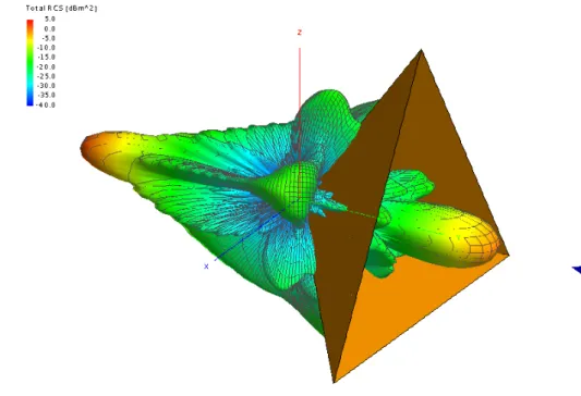
4.3 3D representation of bistatic RCS . . . 38

4.4 Aluminium corner reflector prototype . . . 39

4.5 Experimental set-up in the anechoic chamber . . . 39

(14)

4.6 400 single-chirp averaged range profile at each RX channel . . . 42

4.7 Bin 82 amplitude of 400 single-chirp measure (DoA = 0◦) . . . 43

4.8 Bin 82 amplitude of a chirp frame measure (DoA = 0◦) . . . 44

4.9 Position of the reflector for different chirp bandwidths . . . 45

4.10 Range profile for different chirp bandwidths . . . 45

4.11 Range-Doppler map of the anechoic chamber set-up . . . 47

4.12 Phase of range-bin 82 along the 400 single chirps . . . 48

4.13 Phase of range-bin 82 along a frame of chirps . . . 48

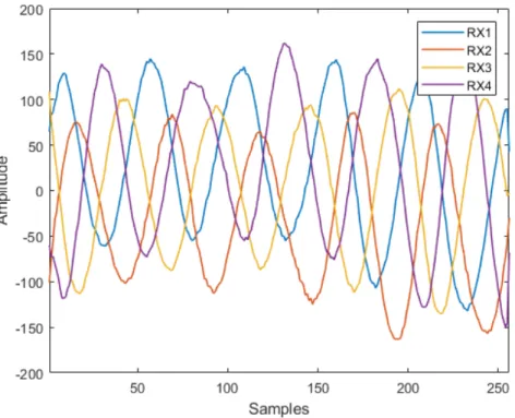
4.14 Phase of each RX channel for TX 1 . . . 49

4.15 Phase response over a frame without system drift . . . 50

4.16 Virtual 7 element array . . . 53

4.17 Range versus angle map of the anechoic chamber (DoA = 24◦) . . . 54

4.18 Range versus angle map resolution (DoA = 0◦) . . . 56

4.19 Comparison of spatial spectra at resolved position of the reflector . . . 57

4.20 XY plot of the chamber scenario (DoA = -45◦) . . . 57

4.21 Field of view of the radar platform . . . 58

4.22 Field of view of the trihedral reflector . . . 58

5.1 Chirp with frequency shift . . . 63

5.2 Target emulator schematic . . . 65

5.3 Single-sideband mixer model . . . 66

5.4 Schematic of the lumped element hybrid coupler . . . 68

5.5 Simulation results of the lumped element hybrid . . . 69

5.6 Simulation results of the transformer-based hybrid . . . 70

5.7 Schematic of the transformer-based hybrid coupler . . . 71

5.8 Lumped and transformer-based hybrid couplers . . . 71

5.9 Range profile with emulated target at 23 metres . . . 73

(15)

List of figures xiii

5.11 Emulator prototype . . . 74

(16)

(17)

List of Tables

1.1 Comparison between available sensing technologies . . . 3

2.1 FMCW expressions summary . . . 18

3.1 Position of antennas on the board . . . 24

3.2 Main chirp parameters . . . 32

3.3 DemoRad capabilities . . . 34

4.1 Measurement signal configuration . . . 40

4.2 Phase drift and velocity error on a 128 chirp frame . . . 50

(18)

(19)

Glossary

The radar field has an extensive vocabulary that sometimes can lead to confusion. In this glossary some words and the usage of some terms in this project are explained.

Terms

• Range and distance Although initially used with different meanings, range meant the round-trip and distance the single trip, both terms are now used in conjunction to refer to the displacement from the radar to the target, in metres.

• TransmittersWithin this project different terminology is used to refer to the transmitter antennas. Either TX ortransmitter can be found in this document.

• ReceiversAs with transmitters, in order to refer to the 4 receiver antennas of the board, either RX,receiver orchannel is used.

Acronyms

• UWB Ultra wide band

• IF Intermediate frequency.

• LO Local oscillator.

• FFTFast Fourier transform.

• DoA Direction of arrival.

• MSPSMegasamples per second.

• SSB Single-sideband (mixer).

• USB/LSB Upper sideband / lower sideband.

(20)

(21)

Chapter 1

Introduction

Although normally linked to military and law enforcement applications due to its development, RADAR is nowadays a widespread solution for civil situations. The term itself was initially coined by the US Navy as an acronym for Radio Ranging and Detection (hereafter written without capitals) and was firstly developed in parallel by Germany, Great Britain and the US, prior to World War II (WWII).

As a short historical introduction to radar one must head back to Christian Hülsmeyer and his Telemobiloskop, an invention patented in 1903 that was aimed to prevent ship collisions in foggy conditions. The invention was based on Heinrich Hertz discoveries on the reflection of EM waves on metallic surfaces. Hülsmeyer is usually credited with the invention of radar eventhough his patents were unknown to the next generation of engineers that developed real military radar deployments in the 30’s [Sar14]. Different events triggered the discovery of radar for each of the different teams working on detection systems, and Rudolph Kühnold (German Navy), Rober Watson-Watt (British Army) and Robert M. Page (US Navy) are considered the developers of radar in their respective countries. The use of German Freya, Würzburg and Seetakt systems and the fast deployment of britishChain Home were key factor for the evolution of WWII, and the need to counterfeit enemy systems lead to huge efforts on microwave technologies research. These efforts made possible all the applications that were developed from the 50’s onwards. Once WWII was ended, parallel to further improvement of military radar, civilian focused applications such as weather forecasting, surveillance for civilian aviation or ship collision avoidance were conceived but technological constraints made these systems unable to be widely marketed. For example, power requirements made portable detection devices almost impossible. In the 70’s, thanks to significant advances, first tests on automotive radar were performed and were the first steps into a whole new field of research that is nowadays trending. Today, connectivity and smart devices drive our lives and are changing the paradigm. The initially sci-fi concept of a self-driven car is now real and relies on the performance of an specific system: radar.

(22)

1.1 Automotive safety

More than 1.2 million people die in traffic accidents each year worldwide making it the main cause of death among young people [WHO15]. At the same time, road accidents are estimated to cost an average of 3% of world’s GDP. In the case of Spain, the total cost (including public health system data) is estimated around 9.25 billion Euro, which means approximately 1% of the country’s gross domestic product [Coo17]. This numbers are a great concern for both governments and the automotive industry: the firsts assume a big part of the overall cost of accidents and automotive industry fears a change on how society conceives cars and their dangers. They do not want to be considered a dangerous means of transportation and it is to be remarked that automotive is one of the biggest industries worldwide; specifically in Spain, where almost 300,000 people are employed in the automotive sector. These fears have been the motive behind investments in advanced security technologies in the last decades and are pushing towards an scenario where there are no automotive-related fatalities. Companies are looking for an equilibrium between investing in security systems, meeting demand of these solutions and getting ready for an expected regulation making these systems mandatory. EU programHorizon 2020, under the slogan2011 - 2020: the decade of action for road safety sets radar sensors and cameras for autonomous driving as a key topic to be funded.

From a historical point of view, as early as in 1970, first solutions started to be developed and new terms such as Long Range Radar (LRR), short range radar (SRR), Blind Spot Detection (BSD) or Lane Change Warner (LCW) were coined. First experimental systems appeared in the early 1970’s but it was not until 1998 that Mercedes-Benz released the 77 GHzDISTRONIC system that was followed in 2006 by DISTRONIC PLUS, the first series-produced automotive radar system. It featured a 77 GHz LRR sensor and two 24 GHz SRR sensors [Mei14]. Since then, most automotive manufacturers have adopted radar systems not only for premium cars but for all their vehicles. New security solutions such as Adaptive Cruise Control (ACC) or Automatic Emergency Braking (AEB) are now possible and suppose a revolution. The afore-mentioned systems are normally referred to as ADAS (Advance driver-assistance systems) and include a vast range of applications that aim to help and guide the driver to avoid accidents and dangerous situations: forward collision avoidance, parking sensors or pedestrian protection systems. The objective behind all this technology is making the vehicle capable of interacting with its surrounding elements to counter human limitations such as reaction times. Although ADAS have since long been a hot topic, it has not been until the last decade that companies have invested large amounts of money, and this has been possible due to the development of new communication technologies that allow the conception of a key idea: connected vehicles. The release of LTE - Advanced and the growing interest and expectations on the so-called 5G have created an internet of things (IoT) fever in which everybody dreams of a near future where all devices are connected: from the fridge to the blinds. This connectivity is actually tangible for

(23)

1.2. Spectrum regulation 3

Sensor Strengths Weaknesses

Infra-red (IR) Low cost. Wide FOV.

Short range designed.

Rain and dust affected. No velocity measurement

Ultrasound (US) Low cost and short range designed. No angular resolution. Noise and wind affected

Laser High directivity. Excellent choice for range

Rain and fog affected

Camera Good FOV. Average max. range. No velocity data

Radar Good under all weather conditions. Range up to 250 m. Good cost.

No object classification.

Lidar Best velocity and range resolution High cost

Table 1.1: Comparison between available sensing technologies

cars and now it is not uncommon that a new car is equipped with a SIM card that allows it to connect to the Internet and recover information. Companies want to exploit this connectivity in order to improve car performance and fulfil clients expectations. Vehicles that communicate with each other and that can drive themselves based both on on-board systems (like radar) and incoming information from the Internet are proposed. This is the actual driver of the automotive market: the need for better and more reliable safety systems that are cheap to deploy.

1.1.1 Available sensing technologies

In order to describe the importance of radar systems applied to automotive situations and the reasons behind choosing it as a key system, a comparison study between other available sensing systems is described. As seen in table 1.1, other solutions for sensing vehicle surroundings include infra-red, ultrasound, lasers, cameras, radar and lidar, and for each of them, different performance metrics have been evaluated, for example, maximum range, field of view (FOV), weather affectation and economical viability.

1.2 Spectrum regulation

Two frequency bands were initially allocated for radar applications: the 24 and the 77 GHz bands. The hardware limitations of the 77 GHz band made it complicated for the development

(24)

Figure 1.1: Radar frequency spectrum allocation

of novel solutions and in the beginning some systems were deployed at the lower band. The 24 GHz band is an unlicensed band that was initially divided in an ISM (Industrial, scientific and medical) band of 250 MHz from 24 to 24.25 GHz and an ultra wide band (UWB) from 21.65 to 26.65 GHz. Although initially dedicated to radar, due to the increasing development of 5G technologies, the ultra wide band was phased out by the ITU, setting the ”sunset date” on 2021 [Ram17]. This decrease in bandwidth made the remaining ISM band unattractive for automotive radar and most solutions have shifted to the higher 77 GHz band. Figure 1.1 depicts the frequency allocation along the two bands.

As it will be shown later on in this project, range resolution and accuracy are inversely proportional to the bandwidth in automotive radar sensors. Thus, the shift from 24 to 77 GHz supposes an improvement of almost a factor 20 in terms of range resolution, as it is proportional to the swept bandwidth, and an improvement in velocity resolution by a factor of 3, as it is inversely proportional to the frequency. However, not only the automotive sector is shifting towards the higher band, also other industrial applications such as industrial liquid-level sensing or UAV (unmanned aerial vehicle) altimeters are being adapted to the new band. From the automotive point of view, the higher band is also interesting in terms of reducing hardware size and because the higher attenuation due to propagation, reduces the potential interferences with other vehicles.

(25)

Chapter 2

Radar theory

In this chapter a theoretical introduction to radar and a thourough explanation of FMCW radar is presented. The three main radar observables: range, velocity and direction of arrival, and other key figures such as the radar cross section, are treated in terms of maximum achievable values and minimum resolution.

2.1 The concept of radar

Imagine the situation of someone throwing a pebble into a well and listening to sound it produces. From the time delay between throwing the pebble and the sound, an approximation of the well’s depth can be made. This simple case might be every child first contact with the radar concept as it is based on the same principle: emitting electromagnetic waves and ”listening” to the echoes coming from objects these waves have collided with. In general, radar systems can provide many observables such as range1, velocity, target size and target angle, and therefore the physical and mathematical foundations that allow this observables has to be introduced. At the same time, radar performance capabilities strongly depend on a wide range of factors such as the emitted waveform or the bandwidth, and hardware limitations such as the physical size of antennas. In order to give an accurate but simple idea of this topics, the two main approaches to radar systems have to be explained.

Initially, the most intuitive approach to the radar concept might be the pulsed one. Emitting an electromagnetic pulse and receiving its echoes seems a rather simple assumption. Range information can then be extracted from time delay or power measures. However, some drawbacks to this approach exist and will be discussed later on in this section. The second approach consists

1

In the radar community, the term range is either used to refer to the whole round-trip distance travelled by the wave or to the real distance at which the target is located. In this project, the intention is to use range and distance as the real position value. Specific cases, if any, will be noted.

(26)

on emitting continuous waveforms so that range information is extracted from the frequency component induced by the time delay when mixing with a reference signal. Different frequency-modulated waveforms are used in continuous wave (CW) systems, such as linear chirp sequences or triangular waveforms. The CW strategy has some drawbacks as will be discussed later on, but its features do fit requirements well. As a first step, before diving into the depths of radar theory, a first essential metric needs to be presented: radar cross section (RCS).

2.1.1 Scattering

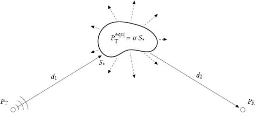
Radar performance lies on the reception of electromagnetic waves reflected from targets and thus the phenomenon of scattering plays a fundamental role. Scattering is a physical process through which some forms of radiation deviate from their trajectory due to meeting obstacles such as singular particles or non-uniformities in the propagation medium. Electromagnetic waves are scattered when they meet with an obstacle and the scattered waves originate from the obstacle’s position. Therefore, any illuminated obstacle appears as a transmitter with its transmit power being directly proportional to the incident (illuminating) power density S. A factor modelling the relation between reflected power and incident power density is called radar cross section (RCS) and denoted byσ. It has units of square meters and depends on the direction of incidence, the direction of scattering, material properties of the obstacle and the wavelength. Figure 2.1 shows a usual bistatic scattering case. Bistatic means that emission and reception locations are not the same and monostatic means that emitter and receptor are at the same position.

Figure 2.1: Bistatic scattering case.

Wavelength influence on RCS is strong as it is responsible for electric size of objects. This means, how big is a target in terms of wavelength λ. Figure 2.2 shows the typical plot of the RCS of a PEC (perfect electric conductor) sphere. See that there are 3 main scattering regions: Rayleigh, resonant or Mie, and optical. The Rayleigh region is the one related to objects that

(27)

2.1. The concept of radar 7

are small in terms of wavelength and the evolution of RCS in this region, is proportional to 1/λ4. The maximum RCS is achieved in the Mie resonant region where the resonating behaviour is due to diffraction and interference between impinging and reflected waves. Finally, RCS converges to an stable value as objects become electrically large and act as a flat surface in terms of reflection. Note that fluctuations of RCS on wavelength may give an idea of another important issue to consider when designing radar systems: operation frequency has an influence on how large targets to be detected can be.

Figure 2.2: Backscattering RCS of a PEC sphere. [Sia18]

2.1.2 Radar range equation

When the scattering phenomenon is considered, the next step to take into account is the path between transmission antenna and the target itself. Recalling Friis transmission formula, incident power density on target can be modeled as follows,

Si=

GPT X

4πr2 (2.1)

whereGis the antenna gain,PT is transmitted power and factor 4πr2 models the surface of

the sphere in which energy is radiated. Given σ =Pscattered/Si, and Aef f = Gλ

2 0

4π (the effective

aperture of the antenna), the received power can be assumed as the propagation of backscattered power, yielding the well-known radar range equation in (2.2).

PR PT = G 2_λ2 0 σ (4π)3_r4 (2.2)

(28)

From the previous equation the first range measurements can be extracted by comparing received and transmitted power. See that path losses and antenna gain are taken into account twice as propagation takes place forth and back.

2.1.3 Pulse radar

The well example at the beginning of this section is an analogy of the so called pulse radar, be-cause the way to achieve range measurement is transmitting pulses and waiting for backscattered echoes to reach the radar. Range is then extracted from the time delay between transmission and reception. The specific features of these systems are mainly bounded by the time duration of the pulse and its repetition frequency. For example, range resolution ∆r, that is the minimum distance between two targets so that they are resolved as different objects, is limited by pulse duration because pulses must not overlap to be correctly resolved. Other well known figures that are inherent to radar systems can be the unambiguous range Runam, the maximum range

at which there is no ambiguity to link transmitted pulses and the respective echoes, that in the case of pulse radar, is limited by the pulse repetition frequency (PRF). In order to tackle some of this limitations, specific techniques such as pulse compression have been developed for pulse radar but these are out of scope in this project because they do not fit automotive sector requirements. Pulse transmission means short high-power bursts combined with echo listening times, which might not be the optimal solution for a highly dynamic environment as the auto-motive. At the same time, achieving high peak power requires from specific hardware (mainly high power oscillators such as klystrons or magnetrons) that can not scale down to fit behind the bumper of a vehicle. Another drawback for the pulse-based approach is that these systems provide hardly any information about target velocity.2 _{These makes this systems suitable for} meteorology and long range surveillance but velocity information is a major requirement in the automotive field. Further explanation on these topics can be found in classical books such as The radar handbook by Merrill Skolnik [Sko08].

2.1.4 Continuous wave radar

The opposite solution to the one based in short pulses is emitting a continuous waveform and thus avoid high-power bursts and the related constraints. The simplest type of continuous wave (CW) radar is one that detects target velocities. The main idea is to transmit a sinusoidal signal and receive the resulting backscattered tone. Because of the Doppler effect, any radial velocity

2_{Since the 1970’s Pulse-doppler radar systems have been developed as an integration of both continuous wave}

and pulsed radar systems. This type of radars are widely deployed in military aircraft and are the actual trend in high budget applications. However they do fall out of scope in the automotive radar field due to size, power and cost limitations.

(29)

2.2. Frequency-modulated continuous-wave radar 9

component present in the target supposes an added Doppler shift to the backscattered signal frequency. Then, when mixed with the transmission reference signal, the received one yields a simple tone at fd. Doppler frequency maps to velocity as in (2.3) considering that factor 1/2

accounts for forth and back propagation, and that fd is Doppler frequency, c0 is the speed of light in vacuum andfc is the carrier frequency.

vr=

fdc0 2fc

(2.3)

See that this mode of operation provides no information about range (there are no time instants to be compared) and that there is neither any information about the target departing or approaching the radar due to the fact that the two possible Doppler frequencies for a specific velocity are the image frequency of each other (fc+fd, fc−fd). They are down-converted to

the same fd absolute value and movement direction cannot be inferred. To solve this situation

an IQ down-converter can be used. Both output signals can be represented as a phasor and the sign of the velocity can be extracted from the rotation direction of it. If the phasor rotates clockwise (mathematically negative) the target departs from the radar, if counter-clockwise (mathematically positive) the target approaches the radar.

Compared to pulsed systems, the system complexity is smaller as there is no need to han-dle high transmission power peaks and additionally, CW systems are highly sensitive to small changes in the observed scenario because phase variations can be detected, what makes them interesting in the field of automotive radar. However, the main drawback is that range informa-tion is lost [Sko08]. Thus, the need for a radar system that can resolve both speed and range is finally approached by a sort of junction between the two previously mentioned schemes.

2.2 Frequency-modulated continuous-wave radar

The reason why CW radar is not able to provide range information is the lack of a time marking strategy that could allow distance calculation and as said before, ranging using pulses is achieved by inferring the distance from time delay between transmitted pulse and echoes. Therefore, a combination of both can be achieved by means of frequency modulated signals such as sawtooth, triangular or stepped frequency. Before going deep into the explanation of the different wave-forms, it is interesting to present the FMCW system. Figure 2.3 shows a rather simple example of such a system, that in essence will consist on a FM signal source, separate transmit and receive antennas and a signal processing chain that will perform the computations explained in the following sections.

Concerning the frequency modulated waveforms, these type of modulations consist on using chirp signals, or in other words, signals whose frequency increases linearly with time. A simple

(30)

ANTENNA TX Mixe r Lowpa s s Filte r I C C DIRECTIONAL COUPLER S awtooth Q I n p u t Spectrum Ana lyz er RF In p u t V o l u m e I In p u t Ex te rn a l Tri g g e r In p u t F re q S p a n A m p Me a s R e s ta rt I n /O u t T ra c e D is p Me a s S e tu p Me a s C n tl Mo d e D e m o B W/ A v g S in g l e Mo d e S e tu p C o u p l e T rig S o u rc e S o u rc e S y s te mP re s e t F il e L o a d Ma rk P rin t S a v e P e a k S e a rc h F u n cMa rk e rS e tu p He l pN e x tZ o o m<>R e tu rn 89 456 123 G Hz MHz k Hz Hz 0k e y 'tra n s l a tio n :. (e n )' re tu rn e d a o b j e c t in s te a d o f s trin g . ><

<

E n try O ff

ANTENNA RX

Figure 2.3: FMCW system sketch

Figure 2.4: Chirp waveform

chirp (see figure 2.4) is a frequency ramp and its instantaneous frequency can be expressed as in (2.4), where B is the swept bandwidth and Tsweep is the time duration of the ramp. A

concatenation of chirps will then form a sawtooth modulation, which is the basis for frequency modulated continuous wave (FMCW) radar operation. Frequency modulation is, additionally, an interesting scheme because by avoiding an envelope modulation, amplifiers can operate in saturation regime without causing major problems.

f(t) =f0+

B

Tsweep

t (2.4)

Before going into the explanation of computation of observables, it is interesting to provide an explanation of the general operation behind FMCW. So, let us assume that there is an static obstacle in front of a chirp-emitting radar. As expected, the emitted wave will travel to the target and due to scattering, will propagate back to the receiving antenna. The chirp will be received and the differences with respect to the emitted one will be a certain delay and attenuation. This attenuation factor is directly related to the RCS of the target and although it is not the main

(31)

topic of this project, it is interesting to point that it is possible to study how do certain objects behave in terms of RCS to find signatures and patterns for object identification.

In this case the focus is on the range information and it will be extracted from the delay factor that appears with respect to the reference chirp. In figure 2.5, a visual explanation of how do chirps provide range information is shown. Due to propagation round-trip delay, the two chirps are in a different point of the slope for a given moment in time. Thus, this difference in instantaneous frequency will yield a single-frequency tone if both signals are mixed, because a mixer outputs the difference and the sum of the radio frequency (RF) and the local oscillator (LO) frequencies3.

2.2.1 Range computation

In the previous straightforward explanation it has been shown that a time delay between two frequency ramps that are mixed will yield a constant frequency tone. This IF tone is related to the chirp ramps as in (2.5) and the round-trip delay is directly related to the distance (R) as

tdelay =c0·R/2. With this, the equations from which the range is extracted are found.

fT X−fRX =fIF = B Tsweep τdelay (2.5) R = c0 fIF Tsweep 2 B (2.6)

Figure 2.5: Relation between delay and IF tone

However, in a real situation it is not so simple to obtain the IF value; the real measured data will yieldsinc-like spectral components at certain bins that refer to range. In the radar module, the IF sinusoid that results from mixing will be sampled and in order to find the value of the

3

(32)

frequency, an FFT (Fast Fourier Transform) will be applied. The FFT algorithm is a fast way to compute the Discrete-Time Fourier Transform that extracts frequency components from a set of ntime-domain samples, and this algorithm is computed by the radar module for each of the received chirps. Ideally for an static target, the desired FFT output would be a Dirac delta at the exact IF frequency. However, the fact that the sinusoid is finite (i.e. windowed in time) will yield a convolution with a sinc function in the frequency domain, the main lobe width of which is directly related to the amount of samples taken from the sinusoid (the time duration of the window). The first zero of thissinc function appears at 1/Twindow and this means that the radar

will only be able to separate frequency components that are at least spaced by ∆f = 1/Twindow.

If the frequency spacing is evaluated into equation 2.5 and noting that Twindow is Tsweep, the

expression for the range resolution is achieved in (2.7).

∆R= c0

2B (2.7)

The assumption until now was that a single static target was present in front of the radar, so range resolution was not really considered in the explanation. However, radar sensors are de-signed to cope with crowded environments and multiple targets in range and thus, the minimum distance at which the radar can distinguish between two targets becomes important. See also that the ability to separate close targets only depends on the swept bandwidth and therefore, larger bandwidths yield better resolutions. This is one of the main triggers for the change to 77 GHz operation frequency as the available bandwidth in that band is 4 GHz.

On the other hand, also the maximum range (also called unambiguous range) is a figure to study and it will be limited by the full-power bandwidth of the analog-to-digital converter of the radar. The ADC will have to sample an IF sinusoid whose frequency will be proportional to the range and in order to avoid aliasing, the Nyquist criteria must be fulfilled. The maximum IF frequency that is resolvable by the radar module will then be fs/2 wherefs is the sampling

frequency of the ADC. If this maximum IF frequency is evaluated in (2.5) the following is obtained:

Rmax =

c0 fs Tsweep

4 B (2.8)

Some novel FMCW solutions have presented systems that do cope with signals for which the Nyquist sampling theorem is not fulfilled. This sparse data approach, for example by using the l1-magic algorithms, has been implemented in some radar systems related to compressive sensing. In a rather simple case of undersampling, for a given unambiguous range of for example 100 metres, some techniques can locate targets at range-chunks of 100 metres as long as the

(33)

reception power requirements are met. This solution falls out of scope in this project but has been found in the literature.

2.2.2 Velocity computation

The previous assumption considered that the target was static, but in case the target is a moving one, how will the radar perform? Will it be able to resolve the velocity of the target? If an static target yields an IF tone due to delay between reference and received chirps, note that for a moving target, this IF tone would be the superposition of two frequency components: the IF related to range and a Doppler component due to radial displacement between radar and target. Thus, the IF that results from the mixing stage can be modelled as in (2.9).

fIF = B tdelay Tsweep ±2 fc v c0 (2.9)

Note that there are two different unknowns and one single equation, what makes the situation unsolvable. From a single chirp IF spectra, the Doppler information cannot be extracted as it is overlapping with the range IF component, but the use of the so-called frame of chirps gives a solution to this problem. The mentioned chirp frame is a set of consecutive chirps that are processed together to resolve both range and velocity. Note that the aim of a FMCW system is continuously transmitting and processing chirps, but at some point, the designer has to define how many of this chirps are going to be processed together (due to processor limitations and/or resolution factors).

Assume that a frame ofN pchirps is emitted and arrives back at the radar module. The result will apparently be the same as before: the frame will be delayed with respect to the reference timing and each of the chirps will yield an IF tone that will be sampled and transformed to frequency domain in order to obtain a range profile. However, the key factor here is the phase of each of the IF tones. In terms of amplitude and frequency, all tones will almost be the same for each of the chirps in the frame, but as the target was moving, the phase of each tone will have changed continuously because the travelled distance has changed in-between chirps. Recall that the Fourier Transform is complex valued, yielding for each of the frequency bins, the amplitude of the sinusoid at that specific frequency (module of the complex number) and the phase of that frequency component. X(k) = N−1 X n=0 x(n)e−j2πkn/N ∠X(k) = arctan Im(X(k)) Re(X(k))

(34)

Therefore, after applying the FFT in range direction (i.e. to thensamples of the IF sinusoid), the different chirps spectra can be rearranged as a matrix, one range profile per column. The matrix will look like the one shown in figure 2.6, having N F F T rows (where N F F T is the amount of bins of the FFT) andN pcolumns. Now, another FFT in the second dimension (each of the rows) can be applied. The output of this transformation is the frequency spectrum related to the phase variations along chirps. Therefore, it is the Doppler spectrum. From this values, now the velocity information can be extracted using (2.3).

Figure 2.6: 2D FFT for Range-Doppler estimation [Sia18]

Mathematically, it is proven that both range and velocity can be jointly computed but some constraints need to be considered. See that what is being recovered from each of the different chirps is the phase at a certain point in time, and thus it can be interpreted as if each chirp is a sample of the time evolution of the phase. As usual, correct sampling involves fulfilling the Nyquist criteria so that there is no loss of information. This means that for a given chirp repetition time (that can be interpreted as the phase sampling frequency) there will be a maximum velocity that can be resolved unambiguously. This maximum detectable velocity is therefore limited to phase changes of up to ±λ/4 in between chirps. It might seem confusing as Nyquist states that at most, the phase variation between two samples can be λ/2 but as radar handles forth and back propagation, a change in the target position ofλ/4 will result in a change of λ/2 in the radar module. Applying the mentioned factors, maximum detectable velocity of a given radar can be stated as in (2.10).

(35)

vmax=

λ

4Tsweep

(2.10)

It is important to note that maximum velocity is bounded by the chirp repetition interval

Tsweep which means that faster chirps can map larger velocities4. However, fast ramps do

require from high quality hardware if the swept bandwidth is to be maintained. For the same PLL ramp generator, decreasing Tsweep would mean sweeping less bandwidth and thus reducing

range resolution; which is the first important trade-off in FMCW radar systems.

On the other hand, the velocity resolution will another time be limited by the amount of chirps that fit into a frame as N p will be the window size. See that the phase variation could be defined as follows, ω= 2 2π v Tsweep λ (2.11)

where the factor 2 takes into account that the wave propagates forth and back. At the same time, the resolution in terms of phase is limited to ∆ω= 2π/Npbecause the minimum resolvable

phase is that which sweeps a whole cycle in an entire frame of chirps. If both expressions are put together, the velocity resolution is defined as in (2.12).

∆v= λ

2Np Tsweep

(2.12)

2.2.3 Direction of arrival computation

As a final point to this FMCW introduction, another important figure on automotive radar systems is to be considered. The described range and velocity joint computation can resolve two targets at the same distance that differ in velocity and these measurements can be performed by having only a pair of antennas: a receiver and a transmitter one. But what if it needs to resolve two targets at the same distance and velocity? This ambiguous situation can only be solved by computing the angular position of each target. See that it is of key importance that a radar sensor that aims to detect road obstacles and possible dangers, can accurately compute the direction of arrival (DoA) of the detected targets. Radars mounted in vehicles do have to create a map of all objects within their field of view in order to asses the aforementioned advanced driving assistance systems (ADAS), and this makes direction of arrival (DoA) computation a must.

4_Here_T

sweepis considered assuming that one chirp starts at the exact moment the previous one finished, which

(36)

As it is presented in many antenna lectures, the angle of arrival of an incident wave can be computed by using an array of antennas. The direction at which the angle can be resolved depends on the axis at which the antennas are spaced. Horizontal arrays can resolve azimuth angles and vertical arrays resolve in elevation. At this point, let us consider the situation shown in figure 2.7, where an electromagnetic wave arrives at an antenna array with a certain angle with respect to the normal of the array base line. See that when the wave arrives to the first antenna, it will have to travel a distancedto the next antenna, which will yield a phase difference between the signal captured by the first and the second elements. This phase difference is related to the distance by means of the phase constant β = 2π/λas follows, where θ is the angle with respect to the normal.

φ=β ∆d=β dsin(θ) (2.13)

Each of theNa antennas in an array, will receive a phase delayed copy of the same frame of

chirps, that will be stored as a receive channel. Thus, each antenna of the array is acting as a sampler in the spatial domain and each of the channels is a sample of the spatial frequency (ν) of the wave. This spatial frequency is a physical variable defined asν= 1/λ, with units of cycles per metre, that defines the periodicity of propagation in space domain, exactly as the frequency (f), in cycles per second, does in time. One can relate time evolution of a periodic oscillation by means of frequency and time, and so can do the same with space evolution in terms of spatial frequency and wavelength.

Figure 2.7: DoA antenna array model [PS18]

(37)

transform of n values in time, the frequency components of the signal were computed. Here, the same transformation holds but considering that index n refers now to spatial positions on a base line, and that the transformation yields the spatial frequency components of the signal. This is a transform to the spatial frequency domain or to the wave number domain if the factor 2π is considered. Therefore, peaks at certain spatial frequencies in this spectrum will convert to incident angles. See that now Na is the amount of samples and the resolution of the DoA

measurement is affected by the windowing effect of sampling. The angular resolution is limited by the length of the antenna array and can be defined as in (2.14).

θres =

λ Na d cos(θ)

(2.14)

See that the angular resolution is defined in a single quadrant because of the geometry shown in figure 2.7. Thus, the angular resolution for a -90 to 90 degree map (two quadrants) will be doubled. Nevertheless, another important figure to study is the maximum field of view of the array. The well-known λ/2 spacing between antennas is the application of the Nyquist sampling theorem to spatial frequency: spatial sampling frequency must be at least 2νto recover unambiguous angles of ±90 degrees, which then yields that the spacing must be at least λ/2. See that,

2π

λdsin(θ)< π→θmax= arcsin

λ

2d

(2.15)

Larger spacings would yield aliasing, thus reducing the total unambiguous field of view. Smaller spacing than half a wavelength would not result in wider angles but would not have a negative effect. However, spacing two antennas less than λ/2 is normally not possible because of physical size limitations. Note that antennas do normally span a length of λ/4 at each side of the phase centre.

As a final summary, table 2.1 groups all radar observables maximum values and resolutions to simplify the reading of this document if equations need to be revisited.

2.2.4 Other trends and solutions

In the previous sections the chirp frame approach to FMCW radar has been presented because it is the most widespread solution within the automotive and industrial sector solutions. However there are other frequency modulated waveforms that also yield very good results. For example, the stepped frequency FMCW consists on chirps that are not continuous in frequency but stepped in small constant steps. Another interesting proposal that was in use before the development of fast ramp FMCW (frame of chirps approach) was the triangular waveform. As it has been shown,

(38)

Radar equation PR PT = G2_λ2 0 σ (4π)3_r4 Range R (m) R= c fIF Tsweep 2 B Range resolution ∆R (m) ∆R= c0 2B

Maximum rangeRmax (m) Rmax = c fs₄T_Bsweep

Velocityvr (m/s) vr= f₂d_fc_c0

Velocity resolution ∆v (m/s) ∆v= ₂ _N λ

p Tsweep

Maximum velocityvmax (m/s) vmax = ₄ _T_sweepλ

Angle of arrival resolution θres (degrees) θres= _N_a _{d cos}λ _(Θ)

Field of view - FOV orθmax (degrees) θmax= arcsin ₂λ_d

Table 2.1: FMCW expressions summary

computing velocity from a single frequency ramp is not possible. However, some applications that can not operate in such a fast chirping scheme could compute velocities from long triangular frequency waveforms. The explanation behind this method is shown in figure 2.8. The delay between up-ramps and down-ramps will be different due to the fact that the Doppler frequency component adds a vertical offset. From this differences, now the range fr and the Dopplerfd

frequencies can be computed as

fr=

1

2(fb(down) +fb(up)) fd= 1

2(fb(down)−fb(up)) (2.16) wherefb is the beat frequency.

(39)

(40)

(41)

Chapter 3

DemoRad evaluation board

In this chapter the DemoRad radar platform from Analog Devices is presented as the platform under test for this project. A detailed description of the main board parameters is given at the same time that some aspects of the data output and the measurement routines that can be performed, are presented.

3.1 Hardware overview

The experimental development of this project is conducted on the DemoRad evaluation board from Analog Devices. This board is an FMCW out-of-the-box radar operating at the 24 GHz band, that features two transmit and four receive antennas and includes a simple software solution for fast deployment. The providers of the internal software of the radar are INRAS, a spin-off company from the University of Linz. The module is initially designed as a demonstrative solution of radar capabilities in the 24 GHz ISM band both in range-Doppler and MIMO (massive input massive output) modes. The hardware architecture of the radar is based on the set of Analog Devices elements for automotive radar, listed below:

• Blackfin BF706 digital signal processor.

• ADF4159 PLL and ramp synthesizer.

• ADF5901 2 channel transmitter.

• ADF5904 4 channel receiver.

• ADAR7251 16 bit, 4 channel analog-to-digital converter.

The overall mode of operation of the different devices is based on the Blackfin module that is used to control the RF frontend and to process the received radar signals from the four

(42)

Figure 3.1: DemoRad platform signal chain

antennas. The fast waveform synthesizer (ADF4159) generates the FMCW transmit signals that are fed to the antennas via the ADF5901 two-channel transmitter. The received signals are then down-converted in the four-channel receiver (ADF5904) and the IF signals are then amplified and sampled at the ADAR7251. The board supports both real-time processing at the DSP or computer access to the data via an USB 2.0 or a CAN interface connection.

The chirp signals are generated in conjunction between the frequency synthesizer and the transmitter voltage controlled oscillator. This chirp signal is used both for transmitting and as a reference for the receiver down-conversion stage. The IF signal is sampled by the ADC and allows three different sampling frequencies: 1, 1.2 and 1.8 MSPS. As it has been presented in section 2.2.1, the sampling frequency of the ADC module is the main boundary for the maximum range of the radar. Figure 3.1 shows the interconnection between the different elements of the platform thus describing the signal chain in the RF front-end.

One important parameter of the signal chain is the transmit power. This value is an integer from 0 to 100 where the maximum output power is 8 dBm. The reference poweer-to-value relation can be found in the transmitter datasheet. In terms of chirp bandwidth, the module has a maximum operation frequency of 24.3 GHz thus enabling a maximum bandwidth of 300 MHz.

3.1.1 Physical parameters and antenna arrangement

The board is mounted on a six-layer 25 millimetre thick Rogers RO-4350 substrate. The dimen-sions of the printed circuit board are 100 x 100 millimetre as shown in figure 3.2. The antennas are mounted at the positions shown at table 3.1 where the central reference point is transmitter

(43)

3.2. Firmware 23

Figure 3.2: DemoRad frontside layout

two (TX2 hereinafter). See that the antenna spacing isλ/2 as was mentioned in chapter 2 and that each of them is an eight element patch antenna fed from the back of the PCB. The addi-tion of serial elements in vertical direcaddi-tion tapers the beamwidth on the E-Plane (i.e. vertical) achieving a narrow vertical field of view. The horizontal field of view is therefore not affected and kept as wide as possible. Figure 3.3 is provided by INRAS [Had15] and specifies the E and H plane gain of a single 8-element antenna. The provided antenna parameters are 13.2 dBi gain, 76.5◦ horizontal and 12.8◦ vertical half power beam-width (HPBW).

In terms of energy consumption, the board needs a supply voltage of 12 Volt and a maximum supply current of 290 mA.

3.2 Firmware

Apart from the software solution by INRAS, a set of Matlab classes are provided with the board in order to allow independent radar software programming. These classes constitute the basis to control the Blackfin DSP and the different configuration parameters of the internal devices. This is done via objects from each of the classes and will be explained in the forthcoming sections. See figure 3.4 for an overview of how classes are connected.

(44)

Antenna Horizontal position (mm) TX 1 -18.654 TX 2 0 RX 1 32.014 RX 2 37.231 RX 3 43.449 RX 4 49.666

Table 3.1: Position of antennas on the board

Figure 3.3: Gain of a single 8-element patch antenna

(45)

3.2. Firmware 25

The communication between the Blackfin and the host computer works through a protected routine namedDemoRadUsb. Therefore, the configuration steps can only be tracked until each of the orders is sent through the USB interface. The provided firmware is based on a mother Matlab class called UsbAdi that defines a set of functions that control direct communication with the USB interface. From this class derives the DemoRad class that initializes the board and defines basic parameters and functions to start and stop operation. The next step is class Adf24Tx2Rx4. This class defines specific operation parameters of the radar (for example, the chirp bandwidth) and contains functions concerning the initialization of the different internal devices and the configuration of the radar operation. In the end, there are three low level classes named DevAdf4159, DevAdf5901 and DevAdf5904 that configure internal specific parameters of the synthesizer, the transmitter and the receiver respectively. In the following subsections an straightforward outline of the classes is given in order to give a rather high-level but complete description of the firmware structure.

3.2.1 UsbAdi

Class UsbAdi is the handle class that serves information directly to the USB interface defined by the DemoRadUsb Mex file. Inside the class, three public properties are defined: UsbOpen, UsbDrvVers and stUsbAdiVers. UsbOpen stores the actual status of the connection with the board and the two Vers properties are fixed values related to the code version. The actual version of the USB interface is 1.1.0.

The class defines a set of key functions in terms of communication with the board: CmdBuild, CmdExec,CmdReadData,CmdRecv,CmdSend,DataRead andData Send. These functions give the specific format to the information that is transferred to the board and also give orders to the board in order to read content from its memory. The bus width of the DSP module is 32 bit and thus all read/write orders have to be translated into a 32 bit-long word containing both operation codes and memory addresses.

3.2.2 DemoRad

The Demorad.m class is the initialization of the DemoRad board and its parent superclass is UsbAdi. In the properties section, the following parameters are defined:

• DebugInf is a boolean parameter that enables the display of messages as a debugging tool, while the radar operates.

• stBlkSize, stChnBlkSize, ChirpSize, CalPage, Rad MaskChn, Rad NrChn and stDemoR-adVers are numerical definitions of the size of the internal strings that need to be handled by the DSP. These are parameters that refer to register sizes and low-level data handling.

(46)

• Rad N = 256 is a very important parameter that defines the amount of samples that the ADC takes from each of the IF tones (i.e. from each of the chirps). This value is fixed in the current framework because of the ADC behaviour, and it will be discussed later on. A deeper study on the hardware architecture of the board would enable the modification of this parameters but falls out of scope in this project.

• F uSca = 0.498/216. FuSca stands for Full Scale and encodes the Full Scale Range of the ADC. This range means the maximum Vpp value that the ADC can handle within its quantification range and is divided by amount of values the converter can quantize. The ADAR7251 module has several operation modes but the one selected in this board is

GADC = 21.98 dB and thus maximum voltage range is 0.498 Vpp1, which divided by 216

yields the voltage value of the least significant bit (LSB). This variable is of key importance as it allows accurate mapping of FFT values to voltage.

• ADR7251Cfg, ADIFMCWCfg, ADICal and ADICalGet are arrays composed of 32 bit long configuration words for different devices on the board. For example, ADR7251Cfg contains the whole register configuration of the ADC in order to set it ready for operation. From each of the 32 bit words, the 16 most significant bits are the register address and the 16 least significant bits are the data to be stored into the registers.

The class also defines a long list of methods but only those strongly related with the project are detailed. The ones that are not explained concern actions such as displaying the board or the DSP status, setting up the SPI configuration or reading information from the EEPROM memory, among others.

• BrdGetChirp is a key function in the radar setup. This function commands the module to send, sample and return the data from a set of chirp signals. The length of the chirp frame is defined by parameters StrtPos and StopPos.

f u n c t i o n Ret = B r d G e t C h i r p ( obj , S t r t Po s n , S t o p P o s n ) S t o p P o s n = obj . I n L i m ( S t o p P o s n , 1 , 1 2 8 ) ; S t r t P o s n = obj . I n L i m ( S t r t P o s n , 0 , S t o p P o s n - 1); D s p C m d = z e r o s (3 ,1); 5 Cod = h e x 2 d e c ( ’ 7 0 0 3 ’ ); D s p C m d (1) = 1; D s p C m d (2) = S t r t P o s n ; D s p C m d (3) = S t o p P o s n ;

Ret = obj . C m d R e a d D a t a (0 , Cod , D s p C m d );

10 Ret = Ret (: , end : -1:1);

StopPosn and StrtPosn are bounded between 0 and 128, being 128 the maximum chirp-frame length. This limitation comes from the physical limitation of the DSP internal 1

(47)

3.2. Firmware 27

memory and the need of transferring it to the computer after taking the measurement. Note that the last step in this function is a backwards reorder of the chirps that are output so that the output array is FIFO structured (the first emitted chirp is at the first position). The code above is given as an example of how do functions in this module look like. The procedure is similar in almost every method involving communication from the computer to the board and consists on building an array containing the command parameters (Cmd) and the operation code that has been fixed inside the encrypted Mex file. In the end, every communication step uses one of the functions defined in the UsbAdi class.

• BrdGetCalDat and BrdGetCalInf are two methods that return the calibration data stored in the EEPROM memory of the DSP. This data is used to allow MIMO angular estimation, and can be re-written if a new calibration is performed.

• Dsp SetMimo enables the MIMO mode of the module. This mode consists on alternating TX 1 and TX 2 for each chirp.

• BrdRst resets the board to its default status. It is required to reset the internal registers after each measurement in order to load different configuration parameters.

3.2.3 Adf24Tx2Rx4

Class Adf24Tx2Rx4 is the child class ofDemoRad and apart from all the inherited content, it defines three public sub-objects namedAdf Rx,Adf Tx andAdf Pll. As private properties, this class specifies default configuration parameters that are needed to initialize the board when it is powered up, although they are reconfigured before each measurement routine. Some of this parameters for example areRf f Strt= 24e9 or Rf f Stop= 24.25e9.

• Constructor Adf24Tx2Rx4 creates 3 objects inside the Adf24Tx2Rx4 object, each one concerning the configuration of the receiver (ADF5904), the transmitter (ADF5901) and the synthesizer (ADF4159).

• RfRxEna enables and powers up the selected channels of the receiver. In normal operation condition, the four channels are powered up.

• RfAdf5904Ini and RfAdf4159Ini are functions that initialise each of the objects of the receiver, transmitter and synthesizer. The initialization of each object is defined inside the corresponding class but in general terms, it consists on generating all the values that need to be loaded in the device registers.

• RfTxEna is the initialization function of the transmitter chip. The input parameters are the transmission channel (TxChn) and transmission power (TxPwr).

(48)

• BrdGetData is the measurement trigger function. By calling BrdGetData, function Brd-GetChirp from classDemoRad is used.

f u n c t i o n Ret = B r d G e t D a t a ( obj )

Ret = B r d G e t C h i r p ( obj , obj . StrtIdx , obj . S t o p I d x ); end

See that BrdGetChirp is called stating StrtIdx and StopIdx. These parameters will be explained in detail in section 3.3.

• RfMeas is a function that requires a more detailed explanation to understand how the DemoRad board works. The code of this function is the following:

f u n c t i o n E r r C o d = R f M e a s ( obj , v a r a r g i n ) E r r C o d = 0; if n a r g i n > 2 s t M o d = v a r a r g i n { 1 } ; 5 if s t M o d == ’ Adi ’ d i s p ( ’ S i m p l e M e a s u r e m e n t M o d e : A n a l o g D e v i c e s ’ ) Cfg = v a r a r g i n { 2 } ; 10 if ~ i s f i e l d ( Cfg , ’ f S t r t ’ ) d i s p ( ’ R f M e a s : f S t r t not s p e c i f i e d ! ’ ) E r r C o d = -1; end if ~ i s f i e l d ( Cfg , ’ f S t o p ’ ) 15 d i s p ( ’ R f M e a s : f S t o p not s p e c i f i e d ! ’ ) E r r C o d = -1; end if ~ i s f i e l d ( Cfg , ’ T R a m p U p ’ ) d i s p ( ’ R f M e a s : T R a m p U p not s p e c i f i e d ! ’ ) 20 E r r C o d = -1; end if i s f i e l d ( Cfg , ’ S t r t I d x ’ ) obj . S t r t I d x = Cfg . S t r t I d x ; 25 end if i s f i e l d ( Cfg , ’ S t o p I d x ’ ) obj . S t o p I d x = Cfg . S t o p I d x ; end 30 f s S e l = [1 , 1.2 , 1 . 8 ] . * 1 e6 ; if i s f i e l d ( Cfg , ’ fs ’ )

[ Val C l k S e l ] = min ( abs ( f s S e l - Cfg . fs )); C l k I n t = 1/ f s S e l ( C l k S e l );

e l s e

(49)

3.2. Firmware 29 C l k I n t = 1 e -6; end % E l o i : the f o l l o w i n g 2 if loops , c h e c k if T R a m p U p t i m e 40 % is l e s s t h a n 260 s a m p l e s in the new s a m p l i n g f r e q u e n c y % ( and T r a m p D o is l e s s t h a n 10) if obj . R f _ T R a m p U p / C l k I n t < 260 w a r n i n g ( ’ A d f 2 4 T x 2 R x 4 : Set T R a m p U p to 260 c l o c k c y c l e s ’ ) 45 Cfg . T R a m p U p = 2 6 0 * C l k I n t ; end if obj . R f _ T R a m p D o / C l k I n t < 10 w a r n i n g ( ’ A d f 2 4 T x 2 R x 4 : Set T R a m p D o to 10 c y c l e s ’ ) 50 Cfg . T R a m p D o = 10* C l k I n t ; end s w i t c h ( C l k S e l ) c a s e 1 % S a m p l i n g f r e q 1 MHz 55 obj . A D R 7 2 5 1 C f g (7) = h e x 2 d e c ( ’ 0 0 0 1 0 0 0 0 ’ ) + 1 0 0 ; % M obj . A D R 7 2 5 1 C f g (8) = h e x 2 d e c ( ’ 0 0 0 2 0 0 0 0 ’ ) + 76; % N obj . A D R 7 2 5 1 C f g (9) = h e x 2 d e c ( ’ 0 0 0 3 2 8 3 3 ’ ); % PLL C o n t r o l obj . A D R 7 2 5 1 C f g ( 1 0 ) = h e x 2 d e c ( ’ 0 1 4 0 0 0 0 0 ’ ) + 3; Cfg . Tp = c e i l ( Cfg . Tp /1 e - 6 ) * 1 e -6; 60 Cfg . T R a m p U p = c e i l ( Cfg . T R a m p U p /1 e - 6 ) * 1 e -6; c a s e 2 % S a m p l i n g f r e q 1.2 MHz obj . A D R 7 2 5 1 C f g (7) = h e x 2 d e c ( ’ 0 0 0 1 0 0 0 0 ’ ) + 1 0 0 0 ; obj . A D R 7 2 5 1 C f g (8) = h e x 2 d e c ( ’ 0 0 0 2 0 0 0 0 ’ ) + 3 0 4 ; 65 obj . A D R 7 2 5 1 C f g (9) = h e x 2 d e c ( ’ 0 0 0 3 1 0 0 3 ’ ); obj . A D R 7 2 5 1 C f g ( 1 0 ) = h e x 2 d e c ( ’ 0 1 4 0 0 0 0 0 ’ ) + 3; Cfg . Tp = c e i l ( Cfg . Tp /5 e - 6 ) * 5 e -6; Cfg . T R a m p U p = c e i l ( Cfg . T R a m p U p /5 e - 6 ) * 5 e -6 ; 70 c a s e 3 % S a m p l i n g f r e q 1.8 MHz obj . A D R 7 2 5 1 C f g (7) = h e x 2 d e c ( ’ 0 0 0 1 0 0 0 0 ’ ) + 1 0 0 0 ; obj . A D R 7 2 5 1 C f g (8) = h e x 2 d e c ( ’ 0 0 0 2 0 0 0 0 ’ ) + 3 0 4 ; obj . A D R 7 2 5 1 C f g (9) = h e x 2 d e c ( ’ 0 0 0 3 1 0 0 3 ’ ); obj . A D R 7 2 5 1 C f g ( 1 0 ) = h e x 2 d e c ( ’ 0 1 4 0 0 0 0 0 ’ ) + 2; 75 Cfg . Tp = c e i l ( Cfg . Tp /5 e - 6 ) * 5 e -6; Cfg . T R a m p U p = c e i l ( Cfg . T R a m p U p /5 e - 6 ) * 5 e -6; o t h e r w i s e end 80 Cfg . C l k I n t = C l k I n t ; Cfg . C l k S e l = C l k S e l ;

(50)

obj . R f _ f S t r t = Cfg . f S t r t ; obj . R f _ f S t o p = Cfg . f S t o p ; 85 obj . R f _ T R a m p U p = Cfg . T R a m p U p ; obj . R f _ T R a m p D o = Cfg . Tp - Cfg . T R a m p U p ; Cfg . T R a m p D o = Cfg . Tp - Cfg . T R a m p U p ; d i s p ([ ’ S a m p l i n g f r e q u e n c y : ’ , n u m 2 s t r ... 90 ( f s S e l ( C l k S e l )/1 e6 ) , ’ M S P S ’ ]) obj . A D I F M C W C f g (9) = C l k S e l ; % E l o i : C o n f i g u r e t i c k s w h i c h are i g n o r e d in s a m p l i n g T i c k s = f l o o r (( Cfg . T R a m p U p + ... 95 Cfg . T R a m p D o )/ C l k I n t ); obj . A D I F M C W C f g (8) = T i c k s - 256 - 1 - 7; % E l o i : The f o l l o w i n g c o m m a n d a p p l i e s A D I 7 2 5 1 C f g and % A D I F M C W C f g to the A D A R ADC m o d u l e . 100 obj . D s p _ S e t A d i D e f a u l t C o n f (); if i s f i e l d ( Cfg , ’ M i m o E n a ’ ) if Cfg . M i m o E n a > 0 obj . D s p _ S e t M i m o ( 1 ) ; 105 end end obj . R f A d f 4 1 5 9 I n i ( Cfg ); 110 E r r C o d = Cfg ; end end end

RfMeas is responsible for setting up the main parameters of the chirp signal that are fixed by the user in the measurement routine. These parameters are TRampUp, TRampDo, Rf fStrt, Rf fStop, fs, Tp, StrtIdx and StopIdx, that stand for the chirp up-ramp and down-ramp time, the initial and end frequency of the ramp, the sampling frequency, the total duration of a chirp and the indices of measurements, respectively. Before loading the configuration to the registers, the completeness of the values is revised. At first, all parameters are double-checked and loaded into the Cfg struct that will be passed to the initialization functions. One interesting parameter to understand is fs or the sampling frequency. As stated in section 3.1, three sampling frequencies are possible: 1, 1.2 and 1.8 MSPS. So, whichever value is entered in the sampling frequency parameter in the measurement value, it will be rounded down to the nearest allowed frequency (see code line 30). After selecting the clock of the system, the function checks if the desiredTRampUp at

(51)

3.3. Measurement software 31

that sampling frequency would yield 260 samples or more. If not, the ramp-up is modified to the minimum value that yields at least 260 samples. At the same time, selecting the sampling frequency involves changing some of the configuration parameters of the ADC module and therefore, the ”switch case” structure is needed. Note that ramp-up time and chirp duration (up-ramp and down-ramp) are rounded so that they are integer valued (code line 59 and 60). Another interesting parameter to take into account is the Ticks variable. Due to the synthesizer response, the chirp ramp is not ideal. There exists some ripple in the beginning of the ramp and also some down-ramp time is needed to let the PLL restart. Because of this, the Ticks value defines how many samples from the total ones taken of the IF tone, need to be discarded, because they are not correct. As said before, the maximum amount of samples per chirp is bounded to 256 because it is the optimal power of two value for the given sampling frequencies and the maximum sweep bandwidth of 300 MHz.

3.2.4 Device classes: DevAdf4159, DevAdf5901 and DevAdf5904

A thorough explanation of the classes themselves falls out of scope in this project as the config-uration of them is low-level. Understanding all the modified parameters would require a deep analysis of the data sheet of each device. In general words, each of the devices has a set of internal registers where different values need to be loaded. For example, the emission power of the transmitter or the low noise amplifier (LNA) gain at the beginning of the receiver signal chain. Inside the classes, a detailed map of all the inner registers of each device is given. The different functions are designed to translate the predefined configuration into 16 bit-long words including masks and register addresses.

3.3 Measurement software

The explanation of the internal components of the radar platform in the previous section is necessary in order to fully understand the measurement routines presented at this point. Firstly, it is interesting to present the hardware constraints that explain the measurement behaviour of the platform under test; in this case, the chirp frame length needs to be considered. To clarify nomenclature as in 2.2.2, a chirp frame is a set of chirps that are emitted one after the other and that are sampled continuously. Thus, the only unused periods that need to be considered are both the synthesizer idle times at the beginning and the down-ramp periods in the end of each chirp. These periods are considered in the ticks variable defined in class Adf24Tx2Rx4. Due to memory handling limitations and the need to perform calculations (i.e. FFT) on the data, the frame length in this platform is bounded to 128 chirps. This is an important figure to consider, as it means that the longest block of coherent data will be 128 times the duration of a

(52)

chirp. With this, two different measurements will be defined: the 128 chirps frame and the single chirp measurements. This last approach can also be called the ”receive and save” measurement because only one chirp is transmitted, sampled and stored. In a single chirp measurement, there will not be coherence between the chirps, but will be of use in terms of characterizing the behaviour of the platform.

3.3.1 Chirp parameters

Once the meaning of a frame is clear, the key parameters of the chirp signal need to be considered. They have been slightly presented in the previous section and are now stated in table 3.2.

Parameter Value Definition

TxPwr 0 - 100 Transmission power. Integer value from 0 - 100.

fs 1e6, 1.2e6 or 1.8e6 Sampling frequency

fStrt 24e9 Start frequency (min. 23.95 GHz)

fStop 24.3e9 Stop frequency (max. 24.3 GHz)

TRampUp 260/fs 260 samples at either sampling frequency

Tp 300/fs 300 total samples at either sampling frequency

N 256 Effective samples per chirp (fixed)

StrtIdx 0 Starting point of the chirp frame

MimoEna boolean Enables MIMO mode

StopIdx 1 - 128 Last chirp to be recorded

TxAntenna 1 - 2 Tx1 or Tx2

NumFrames 1 - inf. Amount of frames to be recorded in a loop

Table 3.2: Main chirp parameters

Note that the chirp bandwidth can be defined as Bchirp = f Stop−f Strt = 300 M Hz

(in this case the maximum available frequency sweep is used) and that N umChirps =

StopIdx−StrtIdx. From the RfMeas function presented in section 3.2.3 it can be seen that the parameters mentioned above, that are needed to initialise the platform, are passed to the function using a struct. Therefore, in the measurement routine the variable Cfg is defined containing all of them but TxPwr, NumFrames and TxAntenna, that are not used in the RfMeas function.