UC Irvine
UC Irvine Previously Published Works
Title
Short-term quantitative precipitation forecasting using an object-based approach
Permalink
https://escholarship.org/uc/item/5p35p8sr
Journal
Journal of Hydrology, 483
ISSN
0022-1694
Authors
Zahraei, A
Hsu, KL
Sorooshian, S
et al.
Publication Date
2013-03-13
DOI
10.1016/j.jhydrol.2012.09.052
License
https://creativecommons.org/licenses/by/4.0/ 4.0
Peer reviewed
eScholarship.org
Powered by the California Digital Library
Short-term quantitative precipitation forecasting using an object-based approach
Ali Zahraei
a,⇑, Kuo-lin Hsu
a,1, Soroosh Sorooshian
a,1, Jonathan J. Gourley
b,2, Yang Hong
c,3,
Ali Behrangi
d,4 aCenter for Hydrometeorology and Remote Sensing (CHRS), The Henry Samueli School of Engineering, Department of Civil and Environmental Engineering, University of California, Irvine, California, E/4130 Engineering Gateway, Irvine, CA 92697, United States
bNOAA/National Severe Storms Laboratory, Norman, Oklahoma, 120 David L. Boren Blvd., Rm. 4745, Norman, OK 73072, United States c
Department of Civil Engineering and Environmental Science, Atmospheric Radar Research Center, University of Oklahoma, Norman, Oklahoma, 120 David L. Boren Blvd., Rm. 4614, Norman, OK, United States
d
NASA Jet Propulsion Laboratory, California Institute of Technology, Climate, Ocean, & Earth Science, 4800 Oak Grove Drive, Pasadena, CA, United States
a r t i c l e
i n f o
Article history:
Received 18 May 2012
Received in revised form 28 September 2012
Accepted 30 September 2012 Available online 10 October 2012 This manuscript was handled by
Konstantine P. Georgakakos, Editor-in-Chief, with the assistance of David J. Gochis, Associate Editor
Keywords:
Short-term quantitative precipitation forecasting
Nowcasting Storm tracking
s u m m a r y
Short-term Quantitative Precipitation Forecasting (SQPF) is critical for flash-flood warning, navigation safety, and many other applications. The current study proposes a new object-based method, named PER-CAST (PERsiann-ForePER-CAST), to identify, track, and nowcast storms. PERPER-CAST predicts the location and rate of rainfall up to 4 h using the most recent storm images to extract storm features, such as advection field and changes in storm intensity and size. PERCAST is coupled with a previously developed precipitation retrieval algorithm called PERSIANN-CCS (Precipitation Estimation from Remotely Sensed Information using Artificial Neural Networks-Cloud Classification System) to forecast rainfall rates. Four case studies have been presented to evaluate the performance of the models. While the first two case studies justify the model capabilities in nowcasting single storms, the third and fourth case studies evaluate the pro-posed model over the contiguous US during the summer of 2010. The results show that, by considering storm Growth and Decay (GD) trends for the prediction, the PERCAST-GD further improves the predict-ability of convection in terms of verification parameters such as Probpredict-ability of Detection (POD) and False Alarm Ratio (FAR) up to 15–20%, compared to the comparison algorithms such as PERCAST.
Ó2012 Elsevier B.V. All rights reserved.
1. Introduction
Short-term Quantitative Precipitation Forecasting (SQPF), or ‘‘nowcasting’’, is important for a number of hydrometeorological applications (Ganguly and Bras, 2003; Afshar et al., 2010). Both Numerical Weather Prediction (NWP) models and extrapolation-based techniques are widely used in SQPF. While these two methods are different in terms of their approaches, they play an effective and complementary role for SQPF (Golding, 1998; Ganguly and Bras, 2003; Wilson et al., 2004; Sokol, 2006; Liang et al., 2010).
Each of these methods has respective strengths and weaknesses (Wilson et al., 2004). Despite NWP models’ applications in weather forecasting and SQPF, they are sensitive to the initial conditions, resolution, and assimilation algorithms (Golding, 1998). With
high-frequency sampling of observations from new generations of sensor networks, the ability of NWP models to provide short-term predictions is substantially improved over the US (Benjamin et al., 2004, 2009). Although there have been significant improve-ments in NWP models and their broad range of applications, they may still have some limitations. For example, NWP models are associated with significant computational cost, which poses limita-tions in terms of spatial domain, resolution, frequency, and the number of ensemble members. Extrapolation-based or ‘‘data-dri-ven-based’’ algorithms, however, are capable of extracting infor-mation from the ever-increasing volume of remotely sensed data and are reported to be capable of producing reliable forecasts with respect to NWP models, especially within a few hours of the anal-ysis time (Dixon and Wiener, 1993; Johnson et al., 1998; Germann and Zawadzki, 2002, 2004; Mueller et al., 2003; Ganguly and Bras, 2003; Chiang et al., 2006; Vila et al., 2008; Zahraei et al., 2010a, 2010b; Sokol and Pesice, 2012).
Several extrapolation-based nowcasting algorithms have been developed for hydrological applications. The Storm Cell Identifica-tion and Tracking (SCIT) algorithm and the Thunderstorm Identifi-cation, Tracking, Analysis, and Nowcasting (TITAN) algorithm are two examples (Johnson et al., 1998; Dixon and Wiener, 1993). Integration of some of these algorithms into the National Weather
0022-1694/$ - see front matterÓ2012 Elsevier B.V. All rights reserved.
http://dx.doi.org/10.1016/j.jhydrol.2012.09.052
⇑ Corresponding author. Present address: NOAA-CREST, United States.
E-mail addresses:[email protected](A. Zahraei),[email protected](K.-l. Hsu),[email protected](S. Sorooshian),[email protected](J.J. Gourley), [email protected](Y. Hong),[email protected](A. Behrangi).
1 Tel.: +1 949 824 9350; fax: +1 949 824 8831. 2 Tel.: +1 405 325 6472; fax: +1 405 325 1774. 3 Tel.: +1 405 325 3644. 4 Tel.: +1 818 393 8657. Journal of Hydrology 483 (2013) 1–15
Contents lists available atSciVerse ScienceDirect
Journal of Hydrology
Service (NWS) Warning Decision Support System (WDSS) has been reported (Lakshmanan et al., 2009).
Pixel- and object-based are two categories of data-driven SQPF algorithms. There have been several proposed pixel-based quanti-tative precipitation estimation and forecasting algorithms (Grecu and Krajewski, 2000; Mecklenburg et al., 2000; Germann and Za-wadzki, 2002; Montanari et al., 2006; Vant-Hull et al., 2008; Beren-guer et al., 2011; Zahraei et al., 2011a, 2012). These algorithms study atmospheric phenomena from an Eulerian, pixel-based per-spective. Object-based quantitative precipitation estimation and forecasting algorithms, which are the main focus of this paper, con-sider storm events as individual objects (Dixon and Wiener, 1993; Hong et al., 2004; Vila et al., 2008).
An object-based algorithm generally includes three steps: (1) storm identification, (2) storm tracking, and (3) storm projection. The identification and matching/tracking of each storm object at the current time (t) with the corresponding storm in the previous time step(s) (e.g.,t1,t2, etc.) is a major challenge for nowcast-ing and storm life-cycle studies. Storms are dynamic in terms of intensity, texture, and geometrical characteristics. They may also split or merge with other storms, which makes the application of tracking algorithms very challenging (Machado and Laurent, 2004). Several object-based storm-tracking methods have been proposed (Lakshmanan et al., 2009), including: (1) storm-matching technique based on centroid positions (Johnson et al., 1998); (2) storm-cell matching based upon the proposed indices of overlap-ping pixels (Morel et al., 1997); and (3) a modified approach where storm tracking and association has been solved as an optimization problem (Dixon and Wiener, 1993).
These tracking techniques have not been without limitations. For example, the centers of mass methods are not robust in pro-cessing complex-shaped objects effectively. The overlapping tech-nique performs well for large storm systems (e.g., Mesoscale Convective Systems, MCSs), in which storm objects are large en-ough to allow sufficient overlap in consecutive time steps (Lakshmanan et al., 2009; Vila et al., 2008). However, for small-scale thunderstorms, they cannot be tracked effectively using over-lapping techniques. Other proposed techniques also assume that storm objects are long-lived and large enough to be associated with previous time steps (Lakshmanan et al., 2009). Although ob-ject-based algorithms are effective for SQPF, they need further improvements. As an example of newly developed object-based nowcasting algorithms, the Forecast and Tracking the evolution of Cloud Cluster (ForTraCC) has been proposed to identify, track, and forecast MCSs (Vila et al., 2008). This nowcasting tool was ap-plied to evaluate MCS evolution up to 120 min with a 30-min inter-val over southern America.
In this study, a new object-based SQPF algorithm capable of tracking and forecasting storms is developed and described. The proposed algorithm, named PERCAST (PERsiann-ForeCAST), can identify and track storms from GOES-IR (infrared) cloud-top long-wave Brightness Temperature (BT) data. The term ‘‘storm’’ presents all atmospheric phenomena with cloud BT less than a specific threshold (e.g., 240 K) and area larger than 256 km2.
The performance of PERCAST is verified against both radar and satellite data and compared with two comparison SQPF models: (1) PERsistence (PER), and (2) WDSS-II (Warning Decision Support System-Integrated Information). The PER assumes that the future rainfall field is equal to the last available scan. The WDSS-II, developed by the National Severe Storm Laboratory (NSSL) and the University of Oklahoma, is frequently used for the identifica-tion, tracking, and nowcasting of thunderstorms (Lakshmanan et al., 2009).
The methodology of the proposed nowcasting model is pre-sented next, followed by applied data sets, case studies, results and verification, conclusions, and appendices.
2. Methodology
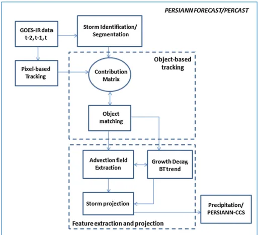
The PERCAST algorithm predicts rainfall rates in the next 4 h (240 min) using infrared satellite imagery (GOES channel 10.8
l
m) with time intervals of about 30 min between two con-secutive satellite observations. Literature shows that a time inter-val of 15–30 min between two observations can be appropriately used to track storm features (Morel and Senesi, 2002; Vila et al., 2008).There are three major steps in PERCAST, as presented inFig. 1: (1) storm identification, (2) storm tracking, and (3) storm projec-tion. The steps are described in detail in the following sections.
2.1. Storm identification (segmentation)
For the object-based nowcasting algorithms, effective storm segmentation is the first step. Mature convective storms can pen-etrate to high altitudes and, therefore, they show overshooting tops and are well associated with colder cloud BT. While BT less than 245 K can satisfactorily identify MCSs, usually the tempera-ture between 228 K and 235 K has been proposed for the summer season, which is based on the assumption that deep convection penetrates in the upper troposphere (Machado et al., 1998; Vila et al., 2008). Vila et al. (2008) proposed a 235 K threshold for MCS nowcasting studies. The proposed PERCAST algorithm would process both mesoscale (e.g., MCS) and small-scale storm events that could not be processed through a single thresholding screen-ing (Lakshmanan et al., 2009). It has been documented that, for cloud and precipitation studies, especially at weather scale, a sin-gle BT threshold is not robust due to seasonal, regional, and cli-matological variability (Adler et al., 1994; Machado et al., 1998). Even multiple threshold techniques have been reported to be problematic for severe storms (Lakshmanan et al., 2009). There-fore, a more advanced segmentation algorithm, called the wa-tershed transform algorithm, has been applied (Roerdink and Meijster, 2001; Lakshmanan et al., 2009; Hong et al., 2004, 2005) (Appendix A).
2.2. Storm tracking and association
By defining contiguous pixels that are segmented in each storm object, matching a storm at the current time (t) with the storm’s corresponding location in the previous time step(s) (e.g., t1, t2, etc.) is a major concern for each nowcasting model. In addition, the PERCAST algorithm needs to track both large- and small-scale events, which create more complexity.
The PERCAST model tracks storms at pixel scale, which connects pixels in two consecutive time steps through the cloud-image advection vectors (Bellerby, 2006). Further, the overlapping pixels within each segmented storm-coverage area from timettot1 are estimated. A backward-forward tracking process connects pix-els in storm objects from timettot1. The contribution/tracking of a storm object fromt1 to another storm at timetcan be cal-culated based on a proposed contribution function, as discussed below.
First, assume that there are two consecutive image objects at time t1 and t, which correspond to the same storm/cloud, where:
Ois an object at timet1, andA(O) is the area ofO,
O0is an object at timet, andA(O0) is the area ofO0.
The contribution function betweenOandO0 (Eq. (1)) is calcu-lated based on the number of pixels (area) being connected from the objectO0at timettoOat timet1 (Morel and Senesi, 2002).
Contribution functionfFO0;Og ¼AðO0Þoriginally fromAðOÞ ¼ ðO\O 0 Þ AðO0 Þ ð1Þ 06 X No:of objectst1 i¼1 FO0;i61 ð2Þ
The contribution function (Eq. (1)) indicates the probability of objectO0contributed from the objectOin the previous time step
t1. Using the pixel-based clouds tracking, PERCAST is able to find the corresponding location of each pixel in the previous time steps (Bellerby, 2006; Zahraei et al., 2011b, 2012). Tracking pixels be-tween times t1 and t extracts the advection of pixels from
t1 tot. Thus, instead of the simple assumption of direct overlap-ping of clouds (e.g.,Vila et al., 2008), the common area along the advection trajectory of pixels covered by two objectsOandO0in two successive time steps can be calculated, which is listed as the numerator in Eq. (1). Because each object at timetis usually linked to one or a few storm object(s) at timet1, the summation of the contribution function for each object at timetwill be be-tween 0 and 1 (Eq. (2)). The value ‘‘1’’ is the case of objects at time
t1 being fully contributed to the specific object at timet, while a value ‘‘0’’ indicates that there was no contribution of objects at timet1 tot that could be a newly generated storm at timet. The object-based overlapping area of the shared pixels of the storm using the advection trajectory in two consecutive time steps is cal-culated for all objects from timet1 (e.g.,O) tot(e.g.,O0). The pro-posed tracking algorithm is able to directly associate the evolution of mesoscale and local convective thunderstorms (Appendix B).
It has been documented that there may be five different situa-tions among the objects, including (1) continuity, (2) spontaneous
generation, (3) dissipation, (4) split, (5) merger, and (6) combinato-rial (Mathon and Laurent, 2001; Vila et al., 2008). The backward-and-forward tracking process using the contribution function makes it possible to consider all situations.
Fig. 2displays the matching of image objects at two consecutive time steps from t1 to t. At time t1, there are five objects, includingA,B,C,D, andE, whereas at timet, there are six storm ob-jects, includingA0,B0,C0,D0,E0, andF0.
2.2.1. Continuity
The common area between two objects from time stepst1 andtimplies that these two objects are from the same storm that has evolved fromt1 to timet, i.e.,Fig. 2a shows that objectsD
andD0are matched. However, it is much more complicated when an object at timet1 is connected with two or more objects at timet. A minimum separation threshold is needed to identify the correct associations for storm objects evolving in time (Morel and Senesi, 2002) (separation threshold –Appendix B).
2.2.2. Generation
Using a backward–forward tracking process, if there is no con-tribution of a storm object from timettot1, the storm object at timetcan be a storm which has just initiated. For objectsE0andF0 at timet, if the contribution function is equal to 0, it means that none of the storm objects from a previous time step are associated with them (E0andF0) (Fig. 2b). Those objects are considered as new storms.
2.2.3. Dissipation
Similar to the generation situation, if there is no contribution of storm objects from time stepst1 tot, the storm can be a dissi-pated one.Fig. 2c shows that objectEat timet1 has disappeared.
Fig. 1.The flowchart of the PERCAST algorithm for precipitation short-term forecasting using satellite information.
2.2.4. Split
When a specific object at timet1 is associated with two or more objects at timet, the result can be the split case. In the case of splitting an object into two or more objects, the largest con-nected object at timetwill be assigned the identification number of the contributed objects from timet1. FromFig. 2d, objectB
could be split intoB0andC0. ObjectsBandB0are matched together. The contribution of objectBinC0is ignored because it is not signif-icant (less than the separation threshold0.25,Appendix B).
2.2.5. Merger
If two or more objects at timet1 are connected to an object at timet, a merger has occurred. For example,Fig. 2c shows that ob-jectsC,B, andEat timet1 might contribute to generating object
C0 at timet. The backward-and-forward tracking process shows that only objectsCandEhave contributed to objectC0, while the portion of object B that has contributed to C0 is not significant (Appendix B).
2.2.6. Combinatorial
The most complicated cases are those in which two or more of the aforementioned situations occur simultaneously, i.e., the case
in which both merging and splitting occur for one specific storm object. For example,Fig. 2c and d shows that object B at time
t1 could split toB0and partly merge to objectC0at timet, while the object-matching process shows that objectBonly significantly contributes to objectB0, and contribution to objectC0is not signif-icant (Appendix B).
2.3. Storm projection
After the storm segmentation/identification and tracking pro-cess, a trajectory for each specific storm from time t to t1,
t2, etc. is assigned. Two different scenarios are used to project (extrapolate) the storm. The first scenario, named PERCAST, uses two consecutive time steps,t1 andt, to extract the storm-advec-tion field (velocity) and uses a fixed velocity to project the storm forward in time (Fig. 3a). The second scenario, called PERCAST-GD, further considers Growth and Decay (GD) along with trends in BT and area of the storm (Fig. 3b). The PERCAST-GD algorithm uses three consecutive time steps,t,t1, and t2, to identify and track storm objects. Given the fact that each storm is now tracked through previous time steps, the projection module can extrapolate the storm. The proposed algorithm projects storms through the following four steps: (1) storm velocity/advection esti-mation, (2) feature extractions such as geometric (area), radiance (BT minimum, BT average), and gradients of features, (3) storm-po-sition prediction, and (4) storm intensity and size prediction. The first two steps extract storm features and variations (gradients of features fromt2 tot1 andt) in addition to each storm advec-tion velocity which will be used by PERCAST-GD for projecadvec-tion. Once the storm is projected, the rainfall algorithm will convert cloud BT to the rate of rainfall. Calculation of each of the four mod-ules will be discussed below.
2.3.1. Storm-velocity estimation
Considering each storm trajectory, the velocityV(C0) of a cellC0 at timetcan be defined using the center of mass location (Morel and Senesi, 2002):
IfC0is a newly generated object at timet, thenV(C0) is the veloc-ity of the nearest cell at timet. If the center of mass of the nearest object is farther than 500 km from the center of mass ofC0, theV(C0) will be considered as 0. Otherwise:
VðC0Þ ¼1
2 CC0
D
t ð3ÞwhereCC0is the distance between the center of mass ofCat time
t1 andC0at timet.
Literatures propose that, instead of calculating the storm-veloc-ity estimation based on the instantaneous speed, it should be cal-culated based on an average of the object trajectories in the previous time steps (e.g., three time steps,t2 tot1 andt1 tot) (Morel and Senesi, 2002). The PERCAST-GD uses the average velocity of objectCmoving from time stept2 tot1 (object
C0) as velocityV(C), and objectC0 att1 moving to the objectC’’ at timetas velocityV(C0). Eq. (4) calculates the velocity of a given object at timet. Two parameters,aandb, show that the velocity is a linear combination of each storm object trajectoryC?C0?C00.
Velocity¼aVðCÞ þbVðC0Þ ð4Þ
The current case studies have revealed that an assumption of
a=b= 0.5 is reasonable.
2.3.2. Storm features extraction
Storm features (e.g., cloud BT/intensity) may change as storms move and evolve. Each convective storm may have three life stages, including initiation, maturity, and dissipation. Newly gen-erated convective storms typically have a strong updraft, and the
Time: t-1
Time: t
(a)
(b)
(c)
(d)
Fig. 2.Schematic representation of two consecutive identified storm objects at timet1 andt. (a) Continuity, (b) generation, (c) dissipation and merger, and (d) split. There are five and six objects at timet1 andt, respectively. The matching process will match the corresponding storms using the proposed object-based tracking algorithm.
BTs at cloud-top become colder and larger in size. Thus, there are important dynamic trends in BT and size. PERCAST-GD considers the aforementioned feature changes and trends. Each of these fea-ture changes might be partially important for an operational algo-rithm intended to provide global short-term precipitation forecasts (Appendix C).
2.3.3. Storm-position prediction
The estimated advection field (velocity) will be applied to pro-ject each storm obpro-ject position. The PERCAST and PERCAST-GD algorithms apply the last 30 min and the average of the last 1-h advection, respectively. The model extrapolates each storm for the next 4 h using the estimated advection field. However, it should be noted that, similar to other algorithms (e.g.,Vila et al., 2008), this nowcasting model has shown its merit in the very short-term forecasting up to2 h.
2.3.4. Storm intensity and size extrapolation
As time passes, storm position, as well as its BT and geometric features at cloud-top, typically change. The PERCAST-GD algorithm extracts storm BT and area changes from previous time steps. When a convective storm grows and becomes colder in terms of BT, the average BT of the object at timet1 is usually lower than the corresponding average BT at timet2. Thus, there are usually cooling (negative) trends in BT. Furthermore, the minimum tem-perature of the growing convective storm is usually lower at time
t1 than its corresponding minimum temperature at timet2. However, there are some exceptions; while the average BT is decreasing, the minimum BT may not be necessarily changing.
Hence, the PERCAST-GD algorithm applies a linear combination of two trends (DBTminandDBTmean), as follows:
D
BT¼cD
BTmeanþdD
BTmin ð5ÞwhereDBTmeanandDBTminare the average and minimumBTtrends,
respectively (Appendix C).canddare weighting parameters. Differ-ent case studies have shown that equal coefficiDiffer-ents (c=d= 0.5) are reasonable.
When convection is growing, the storm usually becomes larger in size and colder in BT. Therefore, the extrapolation algorithm should be able to adjust storm size as well, meaning that each storm has a growth-decay trend in size. The algorithm measures the average of trends to project the storm size (Appendix C) (Fig. 3b). This trend will be applied at the first extrapolated time step (t+ 1), and then will be reduced linearly to about zero from
t+ 2 tot+ 8 to avoid unreasonable values (Scofield et al., 2004). In addition, each object should not grow larger than 100% at each time step (30 min). The accumulated growing factor is also pre-vented from reaching a maximum threshold (e.g., 250–300%) in the next 4 h (Scofield et al., 2004). Similarly, a lower bound is used to control the minimum size that the storm is allowed to shrink.
In summary, the projection procedure includes two different parts, including storm advection, size, and BT prediction. The growth-decay factor can be particularly useful for providing more accurate predictions of changing convective storms.
2.3.5. Rainfall forecast
Using the aforementioned procedure, the PERCAST algorithm will be able to nowcast storms. This paper applies
PERSIANN-Fig. 3.(a) PERCAST, two consecutive time stepst1, andt. The storm grows upward, and it becomes larger and colder,A2<A3, andT2>T3, PERCAST does not consider trends; (b) PERCAST-GD, three consecutive time stepst2,t1, andi. The storm grows upward, and it becomes larger and colder,A1<A2<A3, andT>T2>T3.Vis the 2-D advection vector for the storm,V3= average(V1+V2).
CCS to estimate the rainfall rates of the projected/forecasted storms (Hong et al., 2004). The PERSIANN-CCS algorithm in-cludes a hybrid-segmentation module, a feature-extraction mod-ule, and the ANN module. The first two modules have already been briefly explained. The ANN module is a Self-Organizing Nonlinear Output (SONO) network to classify cloud objects into a similarity-based family of clusters using a Self-Organizing Fea-ture Map (SOFM) (Hsu et al., 1999; Hong et al., 2005; Behrangi et al., 2009). Then, multi-parameter nonlinear functions are cal-ibrated to identify the relationship between the classified cloud objects and their associated precipitation using the Probability Matching Method and the Multi-Start Downhill Simplex optimi-zation technique.
3. Data
The PERCAST-GD model is evaluated using GOES-IR data over a rectangular region between 80°W to 115°W and 32°N to 45°N. The primary forcing data are the full-resolution IR data available from the Climate Prediction Center (CPC) that covers the continental Unites States (CONUS) and adjacent oceans (Janowiak et al., 2001). This data set provides a 0.04°0.04°spatial resolution, a 30-min composite of available GOES-IR imagery that is originally blended from GOES-E and GOES-W satellites. Over the study area, summertime precipitation is dominated by convective storms associated with MCS systems that traverse the Great Plains typi-cally during nighttime hours (Ashley et al., 2003).
t-2
t-1
t
t+2,+60 [min] t+4,120[min]
Cloud BT,
Observation (K)
(a)
(b)
t+2,+60 [min] t+4, +120 [min]
Precipitation Rate
Observation (mm/hr)
(c)
PERCAST-GD
(d)
(e)
PERCAST-GD
[Hits]
(f)
PERCAST
(g)
(h)
PERCAST [Hits]
(i)
Hit Miss False Alarm
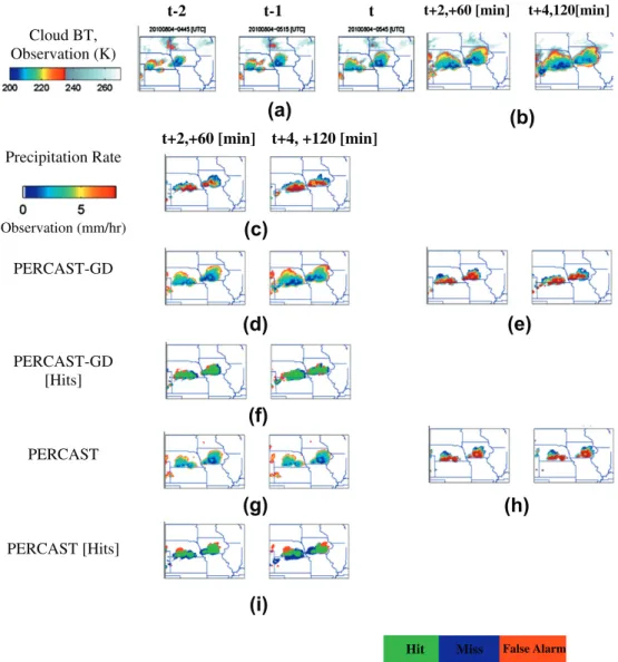
Fig. 4.Case study on 4 August 2010, the most recent cloud BT and observation, as well as the PERCAST-GD and PERCAST algorithms, cloud BT, and rate of rainfall. Hits from predicted vs. CCS and radar Q2 observation. (a) Three consecutive cloud-BT imageries (rainfall >1 mm/h). (b) Cloud-BT observation for +60 (t+ 2) and +120 (t+ 4) [min]. (c) Precipitation rate, CCS observation (t+ 2,t+ 4). (d) Predicted PERCAST-GD (cloud BT) for +60 (t+ 2) and +120 (t+ 4) [min] lead time. (e) PERCAST-GD corresponding predicted rate of rainfall for (d). (f) Hits from PERCAST-GD (e) vs. PERSIANN-CCS observation which is (c). (g) Predicted PERCAST (cloud BT) for +60 and +120 [min] lead time. (h) PERCAST corresponding predicted rate of rainfall for (g). (i) Hits from PERCAST (h) vs. observation (c), less hits more missing compared to (f).
Table 1
PERCAST and PERCAST-GD algorithms, POD and FAR, for the event shown inFig. 4, including +60 and +120 [min] lead time.
Nowcasting POD FAR CSI Nowcasting POD FAR CSI
PERCAST lead time = 60 min 0.57 0.37 0.42 PERCAST lead time = 120 min 0.41 0.51 0.24 PERCAST-GD lead time = 60 min 0.70 0.31 0.53 PERCAST-GD lead time = 120 min 0.63 0.42 0.38
Rainfall estimates from the NEXRAD-based National Mosaic and QPE system (Q2;Zhang et al., 2011) are used for comparison and evaluation of the proposed algorithms. Q2 is a state-of-the-art rainfall estimation system which has significantly mitigated the ef-fects of non-weather contaminants, such as insects, anomalous propagation, and ground clutter and mosaics rainfall estimates into 0.01°0.01°grids every 5 min (Lakshmanan et al., 2007; Vasiloff et al., 2007). For the purposes of this study, the Q2 data have been resampled to the IR satellite resolution.
4. Results
Both PERCASST and PERCAST-GD nowcasting scenarios have been verified vs. both satellite-based observed rainfall (PERSI-ANN-CCS) and ground-based radar rainfall observation. As it was mentioned the proposed model estimate rainfall using projected storms and PERSIANN-CCS. Thus, there are two sources of uncertainty regarding the storm projection and
rain-Fig. 5.Four selected severe storms, GOES-IR observations: (a) Event 1: 20090508-1200 [UTC], (b) Event 2: 20090609-1800 [UTC], (c) Event 3: 20100614-0600 [UTC], and (4) Event 4: 20100623-0450 [UTC] (Unit: Brightness Temperature = K).
fall estimation. To discriminate different errors, the PERSIANN-CCS observations are also compared with the radar-observed rainfall (Q2).
Five performance measures are used for verification of PER-CAST-GD including: (1) Correlation Coefficient (CC), (2) Probability of Detection (POD), (3) False-Alarm Ratio (FAR), and (4) Critical Success Index (CSI) and (5) Odds ratio. They measure the agree-ment between forecast (F) and observation (O) (Legates and McC-abe, 1999; Grecu and Krajewski, 2000; Hogan et al., 2009).Grecu and Krajewski (2000)stated that POD, FAR, and CSI are better met-rics for pattern matching. POD shows the ability of the forecasting algorithm in prediction of rainy/non-rainy pixels, based upon pre-defined thresholds. FAR indicates instances in which the storm is predicted while there is no storm. CSI shows how well the pre-dicted storm corresponds to the observed storm. Hogan et al. (2009)also indicated that POD and FAR have limitations in charac-terizing forecasting skill.Stephenson (2000)represents the odds ratio as a complementary verification measure.
5. Models evaluation
The efficacy of both SQPF scenarios, PERCAST and PERCAST-GD, is evaluated with four case studies. The first case study evaluates a single convective storm event. The second case study shows the application of the proposed model to nowcast four severe storm events. The third evaluation is based on average monthly forecast-ing skill. Estimations from PERCAST and PERCAST-GD algorithms with forecasting lead times up to 240 min using the entire month of May 2010 are evaluated over the entire study area. The fourth evaluation covers five successive months May, June, July, August, and September 2010. The comparison and evaluation of the pro-posed algorithm is conducted over the entire study region for storms greater than 256 km2.
5.1. Case Study I: Evaluation for a single event
Fig. 4displays the application of both PERCAST and PERCAST-GD algorithms for an event on 5:45 UTC 4 August 2010, over the
Midwest US. Fig. 4a shows three consecutive time steps of GOES-IR cloud imagery (BT) in which two separate convective activities start growing at the same time.Fig. 4b displays the next two time steps (t+ 2 andt+ 4), including +60 min and +120 min cloud BT observations, respectively.Fig. 4c illustrates the corre-sponding precipitation rate estimated from PERSIANN-CCS for the storms depicted inFig. 4b.Fig. 4d gives the projected storm using PERCAST-GD, andFig. 4e provides the PERCAST-GD corre-sponding predicted rainfall.Fig. 4f shows the hit, missing, and false alarms with the PERCAST-GD forecast compared with PERSIANN-CCS observations.Fig. 4g displays the projected storm using the PERCAST algorithm, andFig. 4h gives the PERCAST corresponding
Table 2
Information for four storms/events during 2009–2010, including time, length, and states damaged by the storm. The last three columns show if the storms had severe winds, flash flooding, and/or tornados.Source:National Climate Data Center;ncdc.noaa.gov.
Event Time [mm/dd/yy] Length [h] States Severe wind Flash flood Tornado
1 05/08/09 18 KS, MO, KY, VA Yes Yes Yes
2 06/[09–10]/09 18 KS, MO Yes Yes Yes
3 06/[13–14]/10 24 OK, KS Yes Yes Yes
4 06/[22–23]/10 21 NE, SD, IA, WI Yes Yes Yes
Table 3
POD, FAR, and CSI, for four selected storms using PERCAST-GD, PERCAST, WDSS-II, and PER models vs. PERSIANN-CCS observation. Lead time +30 min.
Model +30 (min)
Index Event 1 Event 2 Event 3 Event 4 PERCAST-GD POD 0.65 0.68 0.59 0.54 FAR 0.39 0.37 0.46 0.49 CSI 0.40 0.42 0.33 0.32 PERCAST POD 0.59 0.62 0.5 0.5 FAR 0.44 0.44 0.49 0.53 CSI 0.34 0.36 0.27 0.25 WDSS POD 0.56 0.58 0.48 0.46 FAR 0.45 0.46 0.54 0.55 CSI 0.31 0.32 0.21 0.19 PER POD 0.48 0.51 0.46 0.41 FAR 0.49 0.53 0.56 0.58 CSI 0.22 0.21 0.19 0.16 Table 4
POD, FAR, and CSI, for four selected storms using PERCAST-GD, PERCAST, WDSS-II, and PER models vs. PERSIANN-CCS observation. Lead time +60 min.
Model +60 (min)
Index Event 1 Event 2 Event 3 Event 4 PERCAST-GD POD 0.58 0.6 0.54 0.44 FAR 0.44 0.48 0.43 0.52 CSI 0.32 0.32 0.27 0.2 PERCAST POD 0.49 0.52 0.44 0.39 FAR 0.52 0.6 0.56 0.57 CSI 0.25 0.22 0.18 0.16 WDSS POD 0.43 0.47 0.41 0.38 FAR 0.54 0.59 0.59 0.62 CSI 0.2 0.18 0.16 0.14 PER POD 0.34 0.34 0.36 0.3 FAR 0.6 0.66 0.63 0.68 CSI 0.11 0.09 0.12 0.08
Fig. 6.The Correlation Coefficient (CC) vs. lead time [min] on average for May 2010. The PERCAST + Growth–Decay (GD) algorithm, the PERCAST, the WCN/WDSS-II, and PERsistency (PER) have been plotted. The PERCAST-GD prediction vs. the Q2 radar data is also plotted. The PERSIANN-CCS vs. the Q2 radar shows the application of the rain-conversion algorithm compared to the radar observation. Bars show the minimum, maximum, and average values of the correlation coefficients for May 2010, for PERCAST-GD. The first forecasting time (lead time) ist+ 1 = +30 (min).
predicted rainfall.Fig. 4i shows the hit, missing, and false alarms with the PERCAST forecast compared with PERSIANN-CCS observa-tions. A comparison ofFig. 4e and h shows that the PERCAST algo-rithm predicts storm advection based on the storm movement from time steps t and t1 reasonably well, whereas the PER-CAST-GD predicts both storm advection and convection growth more accurately, as it is designed to do.
ConsideringFig. 4a–i andTable 1, the PERCAST-GD could more accurately forecast advection and evolution of the growing convec-tive activities; for example, comparingFig. 4f and i shows that the POD of PERCAST-GD and PERCAST in lead time of 120 min are 63% and 41%, respectively. Therefore, the PERCAST-GD may be consid-ered a relatively more reliable precipitation forecasting tool, par-ticularly for convective dominant events/seasons.
5.2. Case Study II: Very short term severe storms nowcasting
The second case study involves the evaluation of the proposed models in nowcasting specific severe storms. Four relatively severe storm events over the contiguous United States (CONUS) area are
selected (Fig. 5). They have produced severe winds, flash floods, or tornadoes (Table 2). All storms have caused either human fatal-ities or significant property damage. The selected storms are fast-evolving with complicated structures, and they all produced in-tense rainfall. In addition, the third storm is a unique, relatively stationary storm producing more than 250 mm of rainfall in less than 6 h over Oklahoma.
Four SQPF models have been used, including PER, WDSS-II, PER-CAST, and PERCAST-GD. WDSS-II works with a modified definition of clustering using size criteria (Lakshmanan et al., 2009). Also, it applies the tracking algorithm proposed by Morel and Senesi (2002)to match storms.
Given the fact that this is an event-based case study, a dynamic window traveling with each storm has been applied. Throughout the storm life cycle, this window moves with the storm and iso-lates it from neighboring events to evaluate the performance of the proposed algorithms for that specific severe storm. Each fore-cast is updated every 30 min (Dt) with new satellite observation, using few consecutive time steps (t= current time) and (tDt,
t2Dt= previous time steps).
Fig. 7.(a) The Probability of Detection (POD) vs. lead time [min] for May 2010, PERCAST, PERCAST-GD, WDSS-II, and PER. The PERCAST-GD algorithm is compared with real-time radar observations. The precipitation estimation algorithm (PERSIANN-CCS) is compared with radar (Q2) data. (b) The False-Alarm Ratio (FAR) vs. lead real-time [min] for May 2010, PERCAST, PERCAST-GD, WDSS-II, and PER. The PERCAST-GD vs. real-time radar observation Q2, and PERSIANN-CCS vs. (Q2) data. (c) The Critical Success Index (CSI) vs. lead time [min] for May 2010, PERCAST, PERCAST-GD, WDSS-II, and PER. PERCAST-GD vs. real-time radar observation Q2, and PERSIANN-CCS vs. radar (Q2) data. (d) Logarithm of Odds ratio vs. lead time [min] for May 2010, PERCAST, PERCAST-GD, WDSS-II, and PER. PERCAST-GD vs. real-time radar observation Q2, and PERSIANN-CCS vs. radar (Q2) data. Bars show the minimum, maximum, and average values of the POD, FAR, CSI, and Log (Odds) for PERCAST-GD. The first forecasting time (lead time) is
t+ 1 = +30 (min).
In Tables 3 and 4, performance of PERCAST-GD, PERCAST, WDSS-II and PER models are compared. According to Tables 3 and 4, the PERCAST-GD shows improved performance in very short-term forecasting (30 and 60 min lead time), and PERCAST and WDSS-II perform in a relatively similar manner. Considering the GD and BT trends and robust advection fields of the convective storms, PERCAST-GD is slightly superior to the comparisons mod-els. Assuming there is a newly generated and growing storm, the applied growth trend could enhance POD of the growing storm. Also, the decay trend minimizes FAR ratio when a convective storm dissipates.
On the other hand, PER which is a control model has shown the worst performance amongst the other models, except for the third storm which is relatively stationary.
5.3. Case Study III: Evaluation of May 2010
The third evaluation focuses on forecasting skill vs. lead time for the entire month of May 2010, over the previously mentioned study domain. WDSS-II, PERCAST, and PERCAST-GD, have been ap-plied with every 30 min update.
Figs. 6 and 7 illustrate the application of the three models against the PERSIANN-CCS rainfall observation, PERCAST-GD vs. Q2 and PERSIANN-CCS vs. Q2 observation which are averaged over
the entire domain for May 2010. The verification measures have been used to show the skill of the SQPF algorithms in the next 4 h (from lead time = +30 min, and every 30 min). It is observed that, in terms of CC, POD, FAR, CSI, and odds ratio statistics, the PERCAST-GD algorithm is relatively more accurate, as compared to both PERCAST and WDSS-II.
In the first couple of minutes of lead time (e.g., +30, +60, etc.), all algorithms perform well. The forecasting ability of extrapolation-based SQPF algorithms decreases with increasing lead time. InFig. 6, considering an acceptable Correlation Coef-ficient (CC) threshold of 35–40%, which is the CC of PERSI-ANN-CCS observation vs. radar Q2 observation (a flat line averaged for the entire spatial–temporal study domain), shows that the PERCAST and PERCAST-GD algorithms are capable of providing effective forecasts for the next 90 and 120 min, respectively.
Fig. 7indicates the superiority of using the PERCAST-GD algo-rithm vs. comparison algoalgo-rithms using POD, FAR, CSI, and the log-arithm of the odds ratio for May 2010. Overall, the proposed PERCAST-GD has provided acceptable forecasts in the first 2 h; after that, all models begin to lose their merit and merge toward each other. In addition, the extended lead time (up to 4 h) reveals that extrapolation-based SQPF models may not have any efficacy after 4 h.
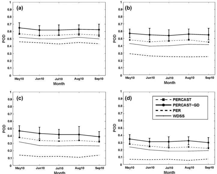
Fig. 8.Probability of Detection (POD) vs. time [month] including May, June, July, August, and September 2010 for rainfall >1 [mm/h], using PERSIANN-CCS as observation. (a) +30 [min] prediction. (b) +60 [min] prediction. (c) +90 [min] prediction. (d) +120 [min] prediction. Bars show the minimum, maximum, and average values of the POD for PERCAST-GD.
As previously mentioned, there are two sources of errors: (1) projection error, and (2) precipitation estimation error of the pro-jected storm. The projection error can be investigated by compar-ing the forecasts with precipitation estimates from PERSIANN-CCS (e.g., PERCAST-GD vs. PERIANN-CCS;Figs. 6 and 7). The precipita-tion estimaprecipita-tion (PERSIANN-CCS) errors due to the conversion of observed brightness temperatures to precipitation rates is identi-fied by comparing PERSIANN-CCS with Q2 estimates, as flat lines shown inFigs. 6 and 7(PERSIANN-CCS vs. Q2), assuming Q2 esti-mates as ‘‘truth’’. Therefore, comparing PERCAST-GD vs. PERSI-ANN-CCS, and Q2 observations, the former only present the error in projection algorithm, while the latter presents the total SQPF er-ror. The gap between the PERCAST-GD vs. Q2 observation and PER-SIANN-CCS vs. Q2 observation (flat line) is assigned to the forecasting algorithm. This difference is initially minor and gradu-ally increases in longer lead time (e.g., after 90–120 min). If the projection algorithm did not have any error, PERCAST-GD vs. Q2 would merge to the flat line.
Figs. 6 and 7also reveal that the main priority of using the pro-posed PERCAST-GD algorithm might be its ability to identify and track local evolving convective storms which are likely to become very severe thunderstorms. These storms might produce signifi-cant amounts of rainfall, while other comparison algorithms have been unable to accurately identify and track them (e.g., WDSS-II).
Adequate tracking of storms is generally considered a prerequisite for accurate SQPF.
In addition, according toGermann et al. (2006), there are a few other important factors affecting forecasting skill, such as the scale dependency. The fact that the selected case studies contain short lifetime and fast-evolving small-scale storms, might be a reason for the relative drop in the forecasting skill after a few minutes of forecasting (e.g.,+30 min lead time).
5.4. Case Study IV: Monthly evaluation (May, June, July, and August 2010)
The previous example showed the forecasting skills of the pro-posed models for a single month (May 2010) vs. lead time, in which there was a decreasing trend in forecasting skill vs. lead time up to 240 min. In those instances where the proposed PER-CAST-GD model performed relatively robust in the first 120 min, models arguably lose their capabilities beyond 120 min. Therefore, this case study evaluates the efficacy of PERCAST-GD over 5 months, for lead time up to 2 h. The verification statistics include POD and FAR at forecast lead times of +30, +60, +90, and +120 min. As shown inFigs. 8 and 9, the +30-min prediction is more reli-able than +60 min and so on. The ability of PERCAST and PERCAST-GD to perform better is due to their ability to more accurately
Fig. 9.False-Alarm Ratio (FAR) vs. time [month] including May, June, July, August, and September 2010 for rainfall >1 [mm/h], using PERSIANN-CCS as observation. (a) +30 [min] prediction. (b) +60 [min] prediction. (c) +90 [min] prediction. (d) +120 [min] prediction. Bars show the minimum, maximum, and average values of the FAR for PERCAST-GD.
identify and track a broader range of storms. Additionally, the con-sistent performance of PERCAST-GD is superior to that of PERCAST and other comparison algorithms. For example,Fig. 8shows that PERCAST-GD outperforms others and is followed by PERCAST for all prediction lead times. Relatively speaking, the PERCAST-GD algorithm improves the predictability of storms (particularly con-vective storms) about 15–20% compared to PERCAST. The GD, as well as the intensity-change components, significantly enhance the capability of the PERCAST-GD algorithm.
Therefore, considering the broad range of global satellite infor-mation, the proposed algorithm may be used as an SQPF tool. The PERCAST-GD algorithm is relatively efficient for operation over the contiguous US and can be extended for precipitation forecasting worldwide.
6. Conclusions
Two object-based algorithms, called PERCAST and PERCAST-GD, suitable for detecting important storm features (e.g., size and intensity trends) were applied and verified. The basic PERCAST algorithm uses two consecutive time steps to track and project the storm, while the PERCAST-GD algorithm considers three previ-ous consecutive time steps, along with the cloud-brightness tem-perature and GD trends. Forecast precipitation fields are estimated based on IR features at cloud-top. Verification results using standard statistical tests demonstrate the superior perfor-mance of PERCAST-GD for short-term forecasts over comparison algorithms.
PERCAST and PERCAST-GD were applied for precipitation fore-casting, and their performances were compared to the WDSS-II and PER using single storm events and 5 months of data during the warm season (May–September) in 2010. Although the WDSS-II algorithm could usually capture storm advection and signifi-cantly outperform the PER model, the verification results based on the standard statistical tests show that both PERCAST and
Fig. A1.(a) GOES-IR observation, 2010618-21:15 [UTC]. (b) Segmented image using watershed transform algorithm.
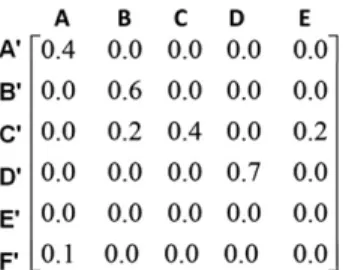
Fig. A2.The contribution matrix, objects at timet1 (A,B, etc.) andt(A0,B0, etc.).
Fig. A3.According to the contribution matrix (Fig. A2), matching corresponding objects. (a) The top-left box belongs to objects at timet1, and the box on the right belongs to objects at timet. Objects are associated fromt1 tot. (b) Storm matching using contribution matrix.
PERCAST-GD perform relatively better. The PERCAST-GD algorithm has the best overall performance.
Using POD, FAR, CSI, the odds ratio, and CC reveals that PER-CAST-GD improves the predictability of convective storms about 15–20% compared to PERCAST. Considering the CC between the PERSIANN-CCS observation and radar observation that is about 35–40% as the threshold, the PERCAST algorithm forecasts well in the first 90 min. Using the same threshold, the PERCAST-GD im-proves predictability by about 30–45 min up to120 min.
While this is the first part of the current research that is more focused on the methodology, and while initial results are encour-aging, more complex and advanced forecasting scenarios (e.g., using cloud life cycles) still need to be investigated. The proposed algorithms need to be comprehensively evaluated (e.g., in cold sea-sons). Efforts are underway by the authors to improve the algo-rithm by testing more scenarios and we will report our findings in future.
Acknowledgements
This research was supported by the Center for Hydrometeorol-ogy and Remote Sensing (CHRS) at the University of California, Ir-vine. Partial financial support was provided by NOAA/NESDIS/ NCDC (prime award NA09NES4400006, NCSU CICS subaward 2009-1380-01), ARO (grant W911NF-11-1-0422) and NASA NEWS (Grant NNX06AF93G). Graduate fellowship support provided by the Hydrologic Research Lab of the US National Weather Service (HRL-NWS) is also greatly appreciated. Part of the research was carried out at the National Severe Storm Lab (NSSL/NOAA), Nor-man, OK. The authors thank Dr. Jeff Kimpel from NSSL for providing the opportunity for collaboration between CHRS and NSSL. Appendix A
A.1. Storm identification/segmentation
Similar to PERSIANN-CCS, the PERCAST model uses a segmenta-tion algorithm named watershed transform (Roerdink and Meij-ster, 2001; Lakshmanan et al., 2009; Hong et al., 2004). This cloud-segmentation algorithm has a few definitions, as follows:
Seed:A seed is a cloud pixel with the relatively coldest pixel of each cold core. A cloud patch starts growing from a cold seed until reaching the terminated condition that can be a size or brightness temperature threshold.
Connectivity:The growing direction that was started from seed points for a 2-D.
Topography of cloud imagery:Assuming that the IR brightness temperature is well correlated with the height of the cloud accord-ing to the physical law of lapse rate, the lower temperature is asso-ciated with higher clouds in the troposphere. In a 3-D overview, the minimum BT represents the cloud-top overshooting points:
s
ðzÞ ¼ dTdz ðA:1Þ
where the actual lapse rate
s
(z) in the atmosphere will be a function of latent heat given to the air by condensation of water vapor. The lapse rate usually ranges in 6–10 K km1.Tandzare temperatureand altitude, respectively.
Segments:Conventionally, a segment is defined as a collection of adjacent pixels having similar values or gradual changes in values. The gradual change of BT is defined as Temperature Interval (TI).
Temperature Interval (TI):It is important how to gradually grow regions from seed points. The TI is a temperature interval to mon-itor the process of patch constitution. TI is estimated from the rela-tionship between cloud BT and cloud height. Larger TI decreases the computation time and increases the undersegmentation of
cloud regions, as opposed to smaller TI, which increases the pro-cessing cost and may oversegment (Hong et al., 2004). PERCAST ap-plies the TI equal to 10.
Topographical Hierarchical Thresholds (THT):Assuming the tem-perature minima as Tmin and the discrimination threshold from
clear sky asTmax, THT is defined as:
THT¼TminþTI i; i¼1;2;. . .;m; where m
¼ jjðTmaxTminÞ=TIjj ðA:2Þ
The THT performs topographically top-down hierarchical thres-holding from the cloud-top coldest core to the discrimination threshold (e.g., 235 K) (Griffith et al., 1978; Xu et al., 1999).
The algorithm primarily locates the coldest seedsTminand then
starts to iteratively expand each seed’s area neighborhood size one at a time by including the border/warmer pixels until touching the separation threshold or the boundary of neighborhood patches. THT conducts a direct growing scheme in which colder pixels/re-gions join first.
Stepwise Seeded Region Growing (SSRG):The seed regions located on the coldest cores of cloud BT will grow up to the warmer region until touching the BT equal to THT =Tmin+ TI. Assuming that the
process completes inmsteps, then all related pixels colder than the specified THTmthreshold are labeled as cloud regions. The pro-cess repeats the previous step until THTmPTmax.
Fig. A1shows the application of the proposed algorithm to seg-ment cloud imageries.
Appendix B
Appendix Bdescribes the storm tracking algorithm.
B.1. Object-based storm tracking and matching
After storm identification/clustering, a tracking algorithm is ap-plied to the identified cells. The object-based tracking algorithm matches the cells/objects from an image to the next one, corre-sponding to the same storm/cloud. As mentioned earlier, the PER-CAST algorithm uses the pixel-based algorithm to track cloud pixels. PERCAST applies the contribution function to associate each storm object at timet1 to the corresponding storms at timet. The contribution function works based on the number of pixels that have been tracked using the pixel-based tracking algorithm. Using a technique that sets all contribution functions in a matrix helps to deal with complicated situations in which hundreds of storms occur simultaneously.
Figs. A2 and A3present this technique.Fig. A2shows the corre-sponding contribution matrix of the storm objects at time steps
t1 andt, andFig. A3illustrates the storm objects from time steps
t1 tot.
Assuming thatn1andn2are the number of identified objects at
time stept1 andt, rows are objects at timetand columns are objects at timet1. There are six rows (n2= 6) and five columns
(n1= 5) (Fig. A2). The hypothetical numbers inside the matrix
rep-resent the contribution function between each two objects at time
t1 andt.
The contribution matrix defines the relationship between ob-jects attandt1. For example, theFA0,A= 0.4 introduces the
con-tribution of the objectA0(timet) from objectA(timet1) at about 0.4 or 40%. This algorithm calculates the contributed area ofA0that actually comes fromA using the pixel-based tracking algorithm. Considering a threshold25% for acceptable contribution function of two storms (betweent1 andt), the 40% contribution is large enough to associate two stormsAandA0.Fig. A3shows the final re-sults in which two storm objectsAandA0are associated. TheF
F0,
-A= 0.1 (Fig. A2) means that object A does not have a major
contribution in the generation of objectF’. The contribution less than the threshold is not acceptable; hence, objectF0is not associ-ated to objectA. Because objectF0is not associated with any object at timet1 (FF0,B= 0,FF0,C= 0,FF0,D= 0,FF0,E= 0), it is a newly
gener-ated storm (Figs. A2 and A3). This matching process eventually associates all storm objects from t1 tot. If an object at time
t1 (e.g., B) is connected with more than one object at time
t1, it may be a split. Conversely, if one object at timet(e.g.,C’) is connected to more than one object at timet1, it may be a merger.
Separation threshold (tsep): The parameter tsepis an important parameter for the tracking-algorithm performance. As mentioned before, the proposed storm-tracking algorithm is defined based on the contribution function of storm objects betweent1 and
t. The contribution function shows what portion (or percentage) of each storm at timetis associated with any of the storms at time
t1. The separation threshold (tsep) is the minimum acceptable contribution function between two objects. As shown by Morel and Senesi (2002), smaller settings oftsepcan lead to some uncer-tainties for events in which storms are moving very close to each other.
Examining the sensitivity oftsepwith respect to different cloud BT and storm size can also be found from prior studies (Vila et al., 2008; Morel and Senesi, 2002). For approximately 75% of the large-scale storms, including MCS and tropical storms, the overlapping ratio is more than 60%. These studies have recommended a separa-tion threshold tsepof about 15–20% for larger-scale atmospheric events (e.g., MCS). For the purpose of this research, a conservative value oftsep= 0.25 is selected to consider both large- and small-scale events.
Appendix C
It describes the storm feature extraction algorithm.
C.1. Storm-feature extraction
After completion of the cloud segmentation and tracking, cloud features should be extracted. The PERCAST-GD model projects each storm based on extracted features. This feature will be applied to estimate how the cloud evolves in the future. The following fea-tures will be used:
(1) Minimum temperature of each cloud object (BTmin).
(2) The minimum-temperature gradient for each storm object using time stepst,t1, andt2.
Considering there are two gradients, Grad (BTmin1) and Grad
(BTmin2), determine how the cloud- minimum BT changes from
time stept1 tot2 andttot1, respectively, and the algo-rithm applies the average of two gradients asDBTmin:
D
BTmin¼ 12fGradðBTmin1Þ þGradðBTmin2Þg ðC:1Þ
(3) Mean temperature of each cloud object (BTmean).
(4) The mean-temperature gradient for each storm object using time stepst,t1, andt2. Considering there are two gradi-ents Grad (BTmean1) and Grad (BTmean2), determine how the
cloud-mean BT changes from time stept1 tot2 andtto
t1, respectively, and the algorithm applies the average of two gradients asDBTmean:
D
BTmean¼ 12fðGradBTmean1Þ þGradðBTmean2Þg ðC:2Þ
(5) Each storm area (A).
(6) Growth and Decay (GD) trend: The PERCAST-GD algorithm uses each storm-size trend to extract GD coefficients. Three consecutive time steps, includingt2,t1, andt, have been applied. DA1 andDA2 are the gradients of each storm object
area from time t2 tot1 and t1 tot, respectively. The algorithm eventually applies DA, which is the average of the storm-object growth and decay trend.DA1andDA2greater than
zero means object growth and vice versa.
Growth—Decay factor¼
D
A¼12f
D
A1þD
A1g ðC:3ÞThe PERCAST-GD projection module applies DA, DTmin, and DTmeanto project each storm object.
References
Adler, R.F., Huffman, G.J., Keehn, P.R., 1994. Global rain estimates from microwave-adjusted geosynchronous IR data. Remote Sens. Rev. 11, 125–152.
Afshar, A., Zahraei, A., Mariño, M., 2010. Large-scale nonlinear conjunctive use optimization problem: decomposition algorithm. J. Water Resour. Plann. Manage. 136 (1), 59–71. http://dx.doi.org/10.1061/(ASCE)0733-9496(2010) 136:1(59).
Ashley, W., Mote, L., Dixon, P.G., Trotter, S.L., Powell, E.J., Durkee, J.D., Grundstein, A.J., 2003. Distribution of mesoscale convective complex rainfall in the United States. Mon. Weather Rev. 131 (12), 3003–3017.
Behrangi, A., Hsu, K., Imam, B., Sorooshian, S., Huffman, G.J., Kuligowski, R.J., 2009. PERSIANN-MSA: a precipitation estimation method from satellite-based multispectral analysis. J. Hydrometeorol. 10, 1414–1429.
Bellerby, T.J., 2006. High-resolution 2-D cloud-top advection from geostationary satellite imagery. IEEE Trans. Geosci. Remote Sens. 44 (12), 3639–3648. Benjamin, S.G., Smirnova, T.G., Weygandt, S.S., Hu, M., Sahm, S.R., Jamison, B.D.,
Wolfson, M.M., Pinto, J.O., 2009. The HRRR 3-km storm resolving, radar-initialized, hourly updated forecasts for air traffic management. In: AMS Aviation, Range and Aerospace Meteorology Special Symposium on Weather-Air Traffic Management Integration, Phoenix, AZ.
Benjamin, S.G., Devenyi, D., Weygandt, S.S., Brundage, K.J., Brown, J.M., Grell, G.A., Kim, D., Schwartz, B.E., Smirnova, T.G., Smith, T.L., Manikin, G.S., 2004. An hourly assimilation-forecast cycle: the RUC. Mon. Weather Rev. 132, 495– 518.
Berenguer, M., Sempere-Torres, D., Pegram, G.G.S., 2011. SBMcast – an ensemble nowcasting technique to assess the uncertainty in rainfall forecasts by Lagrangian extraplation. J. Hydrol. 404 (3–4), 226–240.
Chiang, Y.M., Chang, F.J., Jou, B., Lin, P.F., 2006. Dynamic ANN for precipitation estimation and forecasting from radar observations. J. Hydrol. 334 (1–2), 250– 261.
Dixon, M., Wiener, G., 1993. TITAN: thunderstorm identification, tracking, analysis and nowcasting – a radar-based methodology. J. Atmos. Oceanic Technol. 10, 785–797.
Ganguly, A.R., Bras, R.L., 2003. Distributed quantitative precipitation forecasting using information from radar and numerical weather prediction models. J. Hydrometeorol. 4 (6), 1168–1180.
Germann, U., Zawadzki, I., 2002. Scale-dependence of the predictability of precipitation from continental radar images. Part I: description of the methodology. Mon. Weather Rev. 130 (12), 2859–2873.
Germann, U., Zawadzki, I., 2004. Scale-dependence of the predictability of precipitation from continental radar images. Part II: probability forecasts. J. Appl. Meteorol. 43 (1), 74–89.
Germann, U., Zawadzki, I., Turner, B., 2006. Predictability of precipitation from continental radar images. Part IV: limits to prediction. J. Atmos. Sci. 63, 2092– 2108.
Golding, B.W., 1998. Nimrod: a system for generating automated very short-range forecasts. Meteorol. Appl. 5 (1), 1–16.
Grecu, M., Krajewski, W.F., 2000. A large-sample investigation of statistical procedures for radar-based short-term quantitative precipitation forecasting. J. Hydrol. 239 (1–4), 69–84.
Griffith, C.G., Woodley, W.L., Grube, P.G., Martin, D.W., Stout, J., Sikdar, D.N., 1978. Rain estimation from geosynchronous satellite imagery – visible and infrared studies. Mon. Weather Rev. 106, 1153–1171.
Hogan, R., O’Connor, E., Illingworth, A., 2009. Verification of cloud-fraction forecasts. Quart. J. Roy. Meteor. Soc. 135, 1494–1511.
Hong, Y., Hsu, K., Sorooshian, S., Gao, X., 2004. Precipitation estimation from remotely sensed imagery using an artificial neural network cloud classification system. J. Appl. Meteorol. 43 (12), 1834–1853.
Hong, Y., Hsu, K., Sorooshian, S., Gao, X., 2005. Self-organizing nonlinear output (SONO): a neural network suitable for cloud patch-based rainfall estimation at small scales. Water Resour. Res. 41, W03008. http://dx.doi.org/10.1029/ 2004WR003142.
Hsu, K.L., Gupta, H.V., Gao, X., Sorooshian, S., 1999. Estimation of physical variables from multichannel remotely sensed imagery using a neural network: application to rainfall estimation. Water Resour. Res. 35, 1605–1618.
Janowiak, J.E., Joyce, R.J., Yarosh, Y., 2001. A real-time global half-hourly pixel-resolution infrared dataset and its applications. Bull. Am. Meteorol. Soc. 82 (2), 205–217.
Johnson, J.T., MacKeen, P.L., Witt, A., Mitchell, E.D., Stumpf, G.J., Eilts, M.D., Thomas, K.W., 1998. The storm cell identification and tracking algorithm: an enhanced WSR-88D algorithm. Weather Forecast. 13 (2), 263–276.
Lakshmanan, V., Fritz, A., Smith, T., Hondl, K., Stumpf, G.J., 2007. An automated technique to quality control radar reflectivity data. J. Appl. Meteorol. Climatol. 46, 288–305.
Lakshmanan, V., Hondl, K., Rabin, R., 2009. An efficient, general-purpose technique for identifying storm cells in geospatial images. J. Atmos. Oceanic Technol. 26, 523–537.
Legates, D.R., McCabe Jr., G.J., 1999. Evaluating the use of ‘‘goodness-of-fit’’ measures in hydrologic and hydroclimatic model validation. Water Resour. Res. 35 (1), 233–241.
Liang, Q., Feng, Y., Deng, W., Hu, S., Huang, Y., Zeng, Q., Chen, Z., 2010. A composite approach of radar echo extrapolation based on TREC vectors in combination with model-predicted winds. Adv. Atmos. Sci. 27 (5), 1119–1130. http:// dx.doi.org/10.1007/s00376-009-9093-4.
Machado, L.A.T., Rosso, W.B., Guedes, R.L., Walker, A.W., 1998. Life cycle variations of mesoscale convective systems over the Americas. Mon. Weather Rev. 126 (6), 1630–1654.
Machado, L.A.T., Laurent, H., 2004. The convective system area expansion over Amazonia and its relationships with convective system life duration and high-level wind divergence. Mon. Weather Rev. 132 (3), 714–725.
Mecklenburg, S., Joss, J., Schmid, W., 2000. Improving the nowcasting of precipitation in an Alpine region with an enhanced radar echo tracking algorithm. J. Hydrol. 239 (1–4), 46–68.
Montanari, L., Montanari, A., Toth, E., 2006. A comparison and uncertainty assessment of system analysis techniques for short-term quantitative precipitation nowcasting based on radar images. J. Geophys. Res. 111, D14111.http://dx.doi.org/10.1029/2005JD006729, 12 p.
Mathon, V., Laurent, H., 2001. Life cycle of Sahelian mesoscale convective cloud systems. Quart. J. Roy. Meteor. Soc. 127 (572), 377–406.
Morel, C., Orain, F., Senesi, S., 1997. Automated detection and characterization of MCS using the meteosat infrared channel. In: Proceedings of the Meteorological Satellite Data Users Conference. Brussels, Belgium, EUMETSAT, pp. 213–220. Morel, C., Senesi, S., 2002. A climatology of mesoscale convective systems over
Europe using satellite infrared imagery. I: methodology. Quart. J. Roy. Meteor. Soc. 128 (584), 1953–1971.
Mueller, C., Saxen, T., Roberts, R., Wilson, J., Betancourt, T., Dettling, S., Oien, N., Yee, J., 2003. NCAR auto-nowcast system. Weather Forecast. 18 (4), 545–561. Roerdink, J., Meijster, A., 2001. The watershed transform: definitions, algorithms
and parallelization strategies. Fundam. Inform. 41 (3), 187–228.
Scofield, R., Kuligowski, R., Davenport, C., 2004. The use of the Hydro-Nowcaster for mesoscale convective systems and the Tropical Rainfall Nowcaster (TRaN) for landfalling tropical systems. In: Preprints, Symposium on Planning, Nowcasting, and Forecasting in the Urban Zone, Seattle, WA, American Meteorological Society, 1.4.
Sokol, Z., 2006. Nowcasting of 1-h precipitation using radar and NWP data. J. Hydrol. 328 (1–2), 200–211.
Sokol, Z., Pesice, P., 2012. Nowcasting of precipitation–advection statistical forecast model (SAM) for the Czech Republic. J. Atmos. Res. 103, 70–79.
Stephenson, D., 2000. Use of the ‘‘odds ratio’’ for diagnosing forecast skill. Weather Forecast. 15, 221–232.
Vant-Hull, B., Ba, M., Rabin, R., Mahani, D.S., Kuligowski, R.J., Gruber, A., Smith, S.B., 2008. Transitioning GOES-based nowcasting capability into the GOES-R era. In: Proceedings of the 5th GOES Users’ Conference, New Orleans, LA, pp. 213–220. Vasiloff, S.V., Seo, D.J., Howard, K.W., Zhang, J., Kitzmiller, D.H., Mullusky, M.G., Krajewski, W.F., Brandes, E.A., Rabin, R.M., Berkowitz, D.S., Brooks, H.E., McGinley, J.A., Kuligowski, R.J., Brown, B.G., 2007. Improving QPE and very short term QPF: an initiative for a community-wide integrated approach. Bull. Am. Meteorol. Soc. 88, 1899–1911.
Vila, D.A., Machado, L.A.T., Laurent, H., Velasco, I., 2008. Forecast and tracking the evolution of cloud clusters (ForTraCC) using satellite infrared imagery: methodology and validation. Weather Forecast. 23, 233–245.
Wilson, J.E., Ebert, E., Saxen, T.R., Roberts, R.D., Mueller, C.K., Sleigh, M., Pierce, C.E., Seed, A., 2004. Sydney 2000 forecast demonstration project: convective storm nowcasting. Weather Forecast. 19, 131–150.
Xu, L., Gao, X., Sorooshian, S., Arkin, P.A., Imam, B., 1999. A microwave infrared threshold technique to improve the GOES precipitation index. J. Appl. Meteorol. 38, 569–579.
Zahraei, A., Hsu, K., Sorooshian, S., 2010a. Severe storms nowcasting: using cloud advection field. American Geophysical Union Proceeding, vol. 1. American Geophysical Union, San Francisco, CA, U.S.A, pp. 1141–1146, <http:// adsabs.harvard.edu/abs/2010AGUFM.H33B1141H>.
Zahraei, A., Gourley, J.J., Hong, Y., Lakshmanan, V., Hsu, K., Sorooshian, S., 2010b. Pixel-based very short-term precipitation forecasting for hydrological application. American Geophysical Union Proceeding, vol. 1. American Geophysical Union, San Francisco, CA, U.S.A, pp. 1111–1116, <http:// adsabs.harvard.edu/abs/2010AGUFM.H21E1111Z>.
Zahraei, A., Hsu, K., Sorooshian, S., Behrangi, A., 2011a. Advection-based short-term quantitative precipitation forecasting algorithm using radar and satellite information. American Geophysical Union Proceeding, vol. 1. American Geophysical Union, San Francisco, CA, U.S.A, pp. 2–6, <http:// adsabs.harvard.edu/abs/2011AGUFM.H13I..02Z>.
Zahraei, A., Hsu, K., Sorooshian, S., Behrangi, A., 2011b. Short-term severe storm forecasting using an object-based tracking technique. American Meteorological Conference Proceeding, 18th Conference on Satellite Meteorology, Oceanography and Climatology, vol. 1. American Meteorological Society, New Orleans, LA, U.S.A, pp. 1–8, <https://ams.confex.com/ams/92Annual/ webprogram/Paper201880.html>.
Zahraei, A., Hsu, K., Sorooshian, S., Gourley, J.J., Hong, Y., Lakshmanan, V., Bellerby, T., 2012. Short-term quantitative precipitation forecasting: a Lagrangian pixel-based approach. J. Atmos. Res., 418–434, <http://www.sciencedirect.com/ science/article/pii/S0169809512002219>.
Zhang, J. et al., 2011. National mosaic and multi-sensor QPE (NMQ) system: description, results, and future plans. Bull. Am. Meteorol. Soc. 92, 1321–1338.


![Fig. 7. (a) The Probability of Detection (POD) vs. lead time [min] for May 2010, PERCAST, PERCAST-GD, WDSS-II, and PER](https://thumb-us.123doks.com/thumbv2/123dok_us/10082720.2908320/10.892.90.818.94.695/fig-probability-detection-pod-lead-percast-percast-wdss.webp)