Multiple attribute analysis for deep learning based apparent personality analysis

(1)

Universitat Polit`ecnica de Catalunya

Facultat d’Inform`

atica de Barcelona

Multiple attribute analysis for deep learning

based apparent personality analysis

Ricardo Dar´ıo P´erez Principi

Submitted in part fulfilment of the requirements for the degree of Master of Artificial Intelligence of the FIB UPC

(2)

(3)

Abstract

In this work, we address the problem of apparent personality estimation, meaning the estimation of the impression other people have with respect to someone’s personality.

Apparent personality trait recognition is a complex problem with potential applications in fields such as affective interfaces, social robotics, adaptive marketing and advertising, adaptive tutoring systems, psychological therapy and job recruitment.

Big five traits of personality has emerged as one of the dominant paradigms used in computer based apparent personality estimation. We propose a novel methodology to estimate the fol-lowing personality traits, from a perception perspective: extraversion, agreeableness, openness, conscientiousness, and neuroticism, by including extra sources of information to the primary sources in a multi-modal deep learning fashion. This new information streams are person age, gender, ethnics, emotions, attractiveness and background scene description.

We claim that some of these new extra features are indirectly used by people when estimat-ing others people personality, therefore by includestimat-ing them in the analysis, results should be improved.

With the exception of gender and ethnics, which are given as ground truth, the rest of the features are estimated using different artificial neural networks architectures. As a result a multimodal learning model is presented for apparent personality trait estimation.

En este trabajo, abordamos el problema de la estimación de la personalidad aparente, es decir, la estimación de la impresión que personas tienen con sobre la personalidad de otra persona. El reconocimiento de rasgos de la personalidad aparente es un problema complejo con aplica-ciones potenciales en campos como las interfaces afectivas, robótica social, marketing y publi-cidad adaptativa, sistemas de tutor´ıa adaptativa, terapia psicológica y contratación laboral. Los cinco grandes rasgos de la personalidad han emergido como uno de los paradigmas dom-inantes utilizados en la estimación de la personalidad aparente basada en computadora. Pro-ponemos una metodolog´ıa novedosa para estimar los siguientes rasgos de personalidad, desde

(4)

una perspectiva de percepción: extraversión, amabilidad, franqueza, conciencia y neuroticismo, al incluir fuentes de información adicionales a las fuentes primarias en un modelo de apren-dizaje profundo multimodal. Estas nuevas fuentes de información son edad de la persona, género, etnia, emociones, atractivo y descripción de la escena de fondo.

Afirmamos que algunas de estas nuevas caractersticas adicionales son utilizadas indirectamente por las personas al estimar la personalidad de otras personas, por lo tanto, al incluirlas en el an´alisis, los resultados deben mejorarse.

Con la excepción de género y etnia, que son conocidas, el resto de las caracter´ısticas se estiman utilizando diferentes arquitecturas de redes neuronales artificiales. Como resultado, se presenta un modelo de aprendizaje multimodal para la estimación de rasgos de la personalidad aparente.

KeywordsApparent Personality Estimation; OCEAN model; Deep Convolutional Neural Net-works; Affective interfaces; Social robotics

(5)

Acknowledgements

I would like to express gratefulness to:

• My supervisor, Sergio Escalera, who gave me the opportunity of developing this master thesis and never hesitated in helping me in a very professional and expedite way. His good predisposition for helping, will never be forgotten. I’m deeply grateful.

• My second supervisor, Julio C. S. Jacques Junior, who stood by me and helped with many technical issues that came up during the development of the work. Also for his great suggestions for the conducted experiments, thank you.

• My girlfriend, Bel´en, who supported me in Barcelona and in Buenos Aires. I don’t have enough words to express how much do you mean to my life. Infinite thanks.

• My mother, Adriana, who, always believed in me and in particular during my grade studies of engineering in Buenos Aires and my master studies in Barcelona. Thank you mother.

(6)

(7)

Dedication

I would like to dedicate this master thesis to many people. First, to the person who started my passion for the topic Artificial Intelligence after reading one of his books. Santiago Bilinkis. During the master, I have encountered many interesting, dedicated and good people. Some were teachers, study partners, collegues. I became friend with some of them, and for their friedness, I am deeply grateful. I would like to dedicate this work also to them.

My girlfriend was a key factor by providing me support and love during the whole process. Also a dedication to her.

(8)

Our intuition about the future is linear. But the reality of information technology is exponential, and that makes a profound difference. If I take 30 steps linearly, I get to 30. If I take 30 steps exponentially, I get to a billion.

Ray Kurzweil

(9)

List of Tables

3.1 Information sources, size and description. . . 14

4.1 Experiments performed and which information stream was included in each one of them. V.(Video), A. (Age), G.(Gender), Et. (Ethnics), Em. (Emotions), At. (Attractiveness), P. (Places). . . 29 4.2 Accuracy results over test set. Video (V.), age (A.), gender (G.), ethnics (Et.),

emotions (Em.), attractiveness (At.) and places (P.). Personality traits: ex-traversion (E), agreeableness (A), conscientiousness (C), neuroticism (N) and openness (O). . . 31 4.3 Total number of images for test set for the following population segments:

Male-Asian, Male-Caucasian, Male-AfricanAmerican, Female-Male-Asian, Female-Caucasian and Female-AfricanAmerican. . . 41

(14)

(15)

List of Figures

2.1 Big 5 personality traits. Figure from [Wik18b]. . . 8

3.1 Examples of single frame for some of the clips. . . 12

3.2 Full network architecture including all the extra information streams. . . 15

3.3 Network architecture with only emotions information. . . 16

3.4 Age distribution IMDB + WIKI dataset [RTG16]. . . 18

3.5 Age estimation for some of the images for the First Impression dataset. From top to bottom, from left to right 34, 20, 19 and 21 years old respectively. . . 19

3.6 Most predominant emotion for some images of the First Impressions dataset. From top to bottom, from left to right: sadness, disgust, neutral and fear re-spectively. . . 21

3.7 Beauty scores examples from the paper [LLJ+18]. . . 22

3.8 Average attractiveness factor histogram for the different populations according to ethnicity. First Impressions dataset. . . 23

3.9 Scene prediction results using the VGG16 for randomly selected images of the Places365-Standard dataset. . . 24

3.10 Left: Probability vs CategoryClass (365 classes). Top Right: three most probable classes. Bottom Right: sample frame of sample video. . . 25

(16)

xiv LIST OF FIGURES

4.1 Accuracy over test set. Each block of columns represent one experiment. Nine experiments are represented here, baseline, baseline + age, baseline + gender, baseline + ethnics, baseline + emotions, baseline + attraction, baseline + places, baseline + all - places and baseline + all the features. . . 31

4.2 Personality trait score histogram for each of the five traits (extraversion, agree-ableness, openness, conscientiousness and neuroticism). Ground truth, baseline and baseline + age. . . 33

4.3 Personality trait score histogram for each of the five traits (extraversion, agree-ableness, openness, conscientiousness and neuroticism). Ground truth, baseline and baseline + gender. . . 34

4.4 Personality trait score histogram for each of the five traits (extraversion, agree-ableness, openness, conscientiousness and neuroticism). Ground truth, baseline and baseline + ethnics. . . 35

4.5 Personality trait score histogram for each of the five traits (extraversion, agree-ableness, openness, conscientiousness and neuroticism). Ground truth, baseline and baseline + emotions. . . 36

4.6 Personality trait score histogram for each of the five traits (extraversion, agree-ableness, openness, conscientiousness and neuroticism). Ground truth, baseline and baseline + attraction factor. . . 36

4.7 Personality trait score histogram for each of the five traits (extraversion, agree-ableness, openness, conscientiousness and neuroticism). Ground truth, baseline and baseline + places. . . 37

4.8 Images of videos from the top 20 most accurate image results (extraversion). Baseline (B) vs Improve model (age). Ground truth (GT). 1) GT:0.85046726, B:0.4894714, B+A: 0.78445417; 2) GT:0.3364486, B:0.6353641, B+A: 0.37536004; 3) GT:0.69158876, B:0.43417218, B+A: 0.6644097; 4) GT:0.76635516, B:0.52502894, B+A: 0.75191694. . . 38

(17)

4.9 Images of videos from the top 20 most accurate image results (extraversion). Baseline (B) vs Improve model (gender). Ground truth (GT). 1) GT:0.6635514, B:0.3455922, B+G: 0.65422666; 2) GT:0.85046726, B:0.4894714, B+G: 0.7789629. 38

4.10 Images of videos from the top 20 most accurate image results (extraversion). Baseline (B) vs Improve model (ethnics). Ground truth (GT). 1) GT:0.85046726, B:0.5119484, B+ET: 0.750787; 2) GT:0.7570093, B:0.5042182, B+ET: 0.726135; 3) GT:0.6635514, B:0.3894887, B+ET: 0.608043; 4) GT:0.5794392, B:0.3630559, B+ET: 0.57859546. . . 39

4.11 Images of videos from the top 20 most accurate image results (neuroticism). Baseline (B) vs Improve model (ethnics). Ground truth (GT). 1) GT:0.73333335,

B:0.37926748, B+ET: 0.67457247; 2) GT:0.73333335, B:0.39857784, B+ET: 0.6830916. 39

4.12 Images of videos from the top 20 most accurate image results (conscientious-ness). Baseline (B) vs Improve model (emotions). Ground truth (GT). 1) GT:0.34375, B:0.6799654, B+EM: 0.4277872; 2) GT:0.8645833, B:0.3954034,

B+EM: 0.6284485; 3) GT:0.8333333, B:0.55324715, B+EM: 0.77577513; 4) GT:0.36458334, B:0.6222483, B+EM: 0.4058559. . . 40

4.13 Images of videos from the top 20 most accurate image results (neuroticism). Baseline (B) vs Improve model (emotions). Ground truth (GT). 1) GT:0.43333334, B:0.6767487, B+EM: 0.44482204; 2) GT:0.7777778, B:0.52615035, B+EM: 0.7380421. 40

4.14 Personality trait accuracy by population segment. (Ma-As: Male-Asian, Ma-Ca: Male-Caucasian, Ma-Af: Male-AfricanAmerican, Fe-As: Female-Asian, Fe-Ca: Female-Caucasian and Fe-Af: Female-AfricanAmerican) with age information. . 41

4.15 Personality trait accuracy by population segment. (Ma-As: Male-Asian, Ma-Ca: Male-Caucasian, Ma-Af: Male-AfricanAmerican, Fe-As: Female-Asian, Fe-Ca: Female-Caucasian and Fe-Af: Female-AfricanAmerican) with emotions informa-tion. . . 42

(18)

4.16 Personality trait accuracy by population segment. (As: Male-Asian, Ma-Ca: Male-Caucasian, Ma-Af: Male-AfricanAmerican, As: Female-Asian, Fe-Ca: Female-Caucasian and Fe-Af: Female-AfricanAmerican) with attractiveness information. . . 42

(19)

Chapter 1 Introduction

This chapter introduces the First Impression problem within the scope of Apparent Personality estimation. We cover what motivated us to do this work, main contributions to the research area, and why it claims to be original and a state-of-the-art proposal.

1.1 Motivation and Objectives

When people meet for the first time another person they create a mental image of the person, a ”First Impression” [Wik18c]. This mental image can be made very quickly ([WT06]) based on different features perceived by the observer. Such features include facial expression, physical appearance, body language, clothing, and many more [TMBACGP14]. As an example, pictures taken from the same person but with a different facial expression can change the value of perceived personality traits such as trustworthiness and extroversion [TP14].

Generally speaking, personality prediction can be split into two areas of work, the first one is the correctly recognition of the actual personality traits of people and the second one is estimation of apparent personality traits of others [VM14]. This work focuses on the last one, i.e., apparent personality trait recognition.

The motivation behing this master thesis is to understand how different percieved features, 1

(20)

2 Chapter 1. Introduction

such as emotions, attractiveness, age, gender, etc, can help an automatic system to assess, in a better way, Apparent Personality traits for the First Impression problem.

This master thesis is also motivated by the fact that any of these information sources has been so far jointly analysed in order to address apparent personality trait recognition in a single multimodal framework.

Possible uses for automatic apparent personality trait recognition can be found in areas such as affective interfaces, social robotics, adaptive marketing and advertising, adaptive tutoring systems, psychological therapy and human resourcing, specially in the recruitment process [NGP16].

1.2 Contributions

The paper [GGvGvL16] uses two main information streams to estimate apparent personality traits using videos as input. These information streams are video and audio stream. However, this master thesis focuses on the visual stream only, to investigate and exploit the improvements obtained by using only visual information.

Our contribution to this work is the inclusion of extra information on the baseline pipeline for personality estimation, which demonstrated to be useful for improving accuracy performance. Such features are: emotions, based on facial recognition [Ekm92] [EF71], gender, ethnic, age [RTVG15], attractiveness factor [LLJ+_{18] and background scene information [ZLX}+_14].

In this sense, we will help the model by including all the features above listed. The authors of [JJG+_{18] in their survey of Personality Trait Analysis describe many of the attributes that can}

be a bias in the perception of personality traits.

Some of the features can be quite straight forward to understand why they should be included. For example, emotions play a fundamental role in human cognition and they are an essential field in studies of cognitive sciences like neuroscience or psychology [OJL14]. Human facial

(21)

1.3. Statement of Originality 3

expressions communicates emotions and intentions, therefore, seems to be a valid hypothesis to claim that people tend to estimate personality traits with the aid of perceived emotions. We also claim that perceived people gender, ethnics, age and attractiveness can help apparent personality trait recognition through the inclusion of subjective bias in human perception. Obtained results suggest that personality perception can in fact benefit from these fectures, as detailed in Chapter 4.

To corroborate that, we analyze and discuss the use of different features (age, gender, etc), individually and jointly, when addressing apparent personality recognition.

The proposed model outperformed the baseline model when people emotions information was considered and when all the extra features are jointly considered.

As a final remark, we show that the inclusion of different attributes people generaly use in daily life to perceive others can help apparent personality recognition to achieve better results.

1.3 Statement of Originality

Regarding apparent personality traits estimation, most of the papers only include visual and audio features in the sense that the model takes the images and audio as inputs for different ar-chitectures of Neural Networks (NN) [Wik18a] [SPM+_{16]. Under ChaLearn LAP 2016 challenge}

[Chab], a competition designed to push the state-of-the-art in apparent personality recognition, team NJU-LAMDA [EBEG17] has included verbal content information to his model.

We focus only on the visual aspect of apparent personality estimation which was greatly im-proved by the addition of extra information sources such as gender, ethnics, age, emotions, attractiveness and background scene description, therefore, obtaining a state of the art model. With that regard, we claim the results of apparent personality traits estimation are improved by merging the information provided by the extra features, to the video information channel.

(22)

Chapter 2 Background Theory

In this section we review previous work on personality estimation, starting with solely facial based ones. We set us in context, with the idea of understand how the models have evolved during the past years. Later on, different personality models based on traits are breafly men-tioned, making a particular emphasis in the OCEAN model, also called the Big Five personality model. Finally this chapter will end up with the introduction of the ChaLearn challenge, under which the 2016 First Impression challenge for Apparent Personality recognition took place.

2.1 Previous work

Personality is relevant to any computing area involving understanding, prediction or synthesis of human behavior. All computing domains concerned with personality consider the same three main problems [VM14]:

1. The recognition of the true personality of an individual (Automatic Personality Recogni-tion).

2. The prediction of the personality others attribute to a given individual (Automatic Per-sonality Perception)

(23)

2.1. Previous work 5

3. The generation of artificial personalities through embodied agents (Automatic Personality Synthesis).

During this work, we will deal exclusively with topic number two, Apparent Personality esti-mation.

Among the different people personality theories proposed, trait theory has emerged. Trait theory [CM98] is an approach based on the definition and measurement of habitual patterns of behaviors, thoughts and emotions relatively stable over time. Trait models are built upon human judgments in the form of adjectives that people use to describe themselves and others. For example people with high levels of excitability, sociability, talkativeness, assertiveness, and high amounts of emotional expressiveness can be consider extrovertive.

Those that are against the use of personality trait models argue that the model is purely descriptive and do not correspond to actual characteristics of individuals. One way to discard this criticism is by mentioning that several decades of research and experiments have shown that the same traits appear with regularity across a wide range of situations and cultures, making the personality trait model a valid alternative to characterized psychological phenomena [VM14].

The first models based on visual analysis, for apparent personality estimation, considered the person face as an important source of information for the task. In [WJVS11], they used a static facial information model, to formalize a set of criterion, which is used to make person-ality trait judgments such as aggressiveness, extroversion, likeability, among others. Other authors ([BTMGP12] and [GKS16]) also consider that faces are a rich source of information for apparent personality attribution. They claim that the way people perceieve others might influence on social achievements of the perceived person. For example, attractive people have better mating success, jobs prospects, and earning potential than their less attractive peers. There is a tendency to use global evaluations to make judgments about specific traits, such as attractiveness correlates with perceptions of intelligence.

The importance of First impressions was exceptional presented by the authors of [BT07] who studied how fast judgments of competence based solely on the facial appearance of candidates

(24)

6 Chapter 2. Background Theory

was enough to predict the outcomes of gobernor and Senate elections in the United States in 68.6% and 72.4% of the cases, respectively.

In [JJG+_{18] a comprehensive survey of computer vision based methods for apparent}

person-ality estimation is presented. This work has a very exahustive description of techniques and models for Apparent Personality estimation. The authors also address the problem of apparent personality trait labelling and evaluation. With this regard, it is worth to mention some key issues that should be considered.

It is commonly known that any AI model will learn based on the ground truth information available at training stage, therefore it is expected that the outcome will have the same bias of the ground truth data. Thus, turns out to be necessary to pay attention on how this data is annotated. The author of [JJG+_{18] shows that the validity of such data in case of apparent}

personality recognition can be influence by several factors, such as cultural [WJVS11], social [SYR17], contextual [TP14], gender [MTM+15], appearance [RRGW17], etc. All these factors make the research in this field very challenging. A possible solution for reducing this variability could be to enforce some agreement between annotators in order to make the annotations as reliable as possible.

Biel et al. [BAGP11][BGP13], were the pioneers in studying the Big Five Personality traits from audio visual cues in thin-slices of YouTube personal videos. They took YouTube personal videos as a repository of brief behavioral slices which are a unique medium for selfpresentation and interpersonal perception. They found significant associations between automatically extracted nonverbal cues for several personality judgments. They also explored how different personality traits could be connected to differences in outcome measures of social media participation.

As a side remark, all the work done so far in Apparent Personality trait recognition was in part motivated by the potential interesting applications, all of them based on visual information, in fields greatly diverse such as affective interfaces, social robotics, adaptive marketing and advertising, adaptive tutoring systems, psychological therapy and job recruitment by means of hiring recommendation systems [NGP16].

(25)

2.2. Big Five Personality Model 7

In recent years related topics to First Impression analysis are receiving increasing attention. Those topics are, the already mentioned, hiring recommendation systems and in the field of psychology, depression recognition [PLCO+_{16] [VSS}+_{13] [EPLW}+_16].

As a novel approach to previous works, we will integrate different information sources (gender, ethnics, age, emotions, attractiveness and scene background information) in a single multi-modal, deep learning framework to advance the state-of-the-art in apparent personality recog-nition, integration which, has not been done before.

2.2 Big Five Personality Model

Trait theories of personality have long attempted to describe exactly how many personality traits exist. Earlier theories have suggested a various number of possible traits, including Gor-don Allport’s, with 4,000 personality traits [All37], Raymond Cattell’s with his 16 personality factors [Cat50], and Hans Eysenck’s three-factor theory [EE65]. Between the many traits of Cattell’s theory and the few ones of Eysenck’s theory, many researchers feel that the first model was too complicated and the latter was too limited. As a result, a new theory was developed, and today, many contemporary personality psychologists believe that there are five basic dimen-sions of personality, often referred to as the ”Big 5” personality traits or the OCEAN (Openess,

Conscientiousness, Extraversion, Agreebleness and Neuroticism) model [Nor63] illustrated in figure 2.1.

According to [RC03], the big 5 traits of personality are extraversion, agreeableness, openness, conscientiousness, and neuroticism and can be described as follows.

2.2.1 Openness

This trait features characteristics such as imagination and insight. People who are high in this trait tend to have a broad range of interests. They are curious about the world and other people and eager to learn new things and enjoy new experiences. As well as more adventurous

(26)

Figure 2.1: Big 5 personality traits. Figure from [Wik18b].

and creative. People low in this trait are often much more traditional and may struggle with abstract thinking.

2.2.2 Conscientiousness

Standard features of this dimension include high levels of thoughtfulness, good impulse control, and goal-directed behaviors. Highly conscientious people tend to be organized and mindful of details. They plan ahead, think about how their behavior affects others, and are mindful of deadlines. People with low values of conscientiousness tend to procrastinate important tasks, dislike structure and schedules or fail to complete necessary or assigned tasks.

2.2.3 Extraversion

Extraversion or extroversion is characterized by excitability, sociability, talkativeness, assertive-ness, and high amounts of emotional expressiveness. People who are high in extraversion tend to gain energy in social situations. Being around other people helps them feel energized and excited. For them it is easy to make new friends and they have a wide social circle of friends and acquaintances. People who are low in extraversion (or introverted) tend to be more reserved and on the contrary, have to expend energy in social settings.

(27)

2.3. ChaLearn Challenge 9

2.2.4 Agreeableness

This dimension includes attributes such as trust, altruism, kindness, affection. People with high values of agreeableness tend to feel empathy and concern for other people, they enjoy helping and contributing to the happiness of other people. People who are high in agreeableness also tend to be more cooperative while those low in this trait tend to be more competitive, they don’t care about other people’s interest or problems and sometimes they can even behave in a manipulative way.

2.2.5 Neuroticism

Neuroticism is a trait characterized by sadness, moodiness, and emotional instability. Individu-als who are high in this trait tend to experience mood swings, anxiety, irritability, and sadness. Those low in this trait tend to be more stable and emotionally resilient. They rarely feel sad or depressed and they don’t worry much.

2.3 ChaLearn Challenge

Looking at People (LAP) is a challenging area of research that deals with the problem of recognizing people in images, detecting and describing body parts, inferring their spatial con-figuration, performing action/gesture recognition from still images or image sequences, also considering multi-modal data, among others. Any scenario where a visual or multimodal anal-ysis can be made, is in the field of Looking at People.

Within the frame of ChaLearn, several challenges have been proposed since year 2012 [Chaa]. The challenge for 2016 was First Impressions estimation. And the description of the challenge states that participants have to develop solutions for recognizing personality traits of users in short video sequences. The dataset consists of 10,000 videos of about 15-seconds each collected from YouTube, annotated with personality traits by Amazon Mechanical Turk (AMT) workers

(28)

[AMT]. For each video sample, RGB and audio information are provided, as well as personality impressions (ground truth) values for each of the five traits.

This challenge released the First Impression database for apparent personality recognition, which is the state-of-the-art database on the topic.

The First impression database is used in this master thesis for development, evaluate and compare state-of-the-art models, by using a well known evaluation protocol, defined on the First impression Challenge (described in detail in the next chapter).

(29)

Chapter 3 Methodology

In this section we first describe the dataset used to train, validate and test the proposed models. Later on this section, the different architectures proposed, are described in detail. Finally, given that, the we deal with a multimodal architecture, a detailed description of each of the information streams used is presented.

3.1 Dataset

The original First Impression dataset was released at ECCV 2016 Challenge [PLCO+_{16]. It}

consist in 10,000 videos of 15 seconds each, extracted from more than 3,000 different YouTube high-definition videos of people facing and speaking in English to a camera.

Videos are labeled with traits values (apparent personality). AMT was used for generating the labels [AMT]. A principled procedure was adopted to guarantee the reliability of labels. The considered personality traits were those from the OCEAN model, which is the dominant paradigm in personality research. Each clip has a ground truth label for these five traits represented with a value within the range [0, 1]. Videos show only one person, the scene is clear and the person is facing front at least 80% of the time. Frame rate is not always the same, therefore for a 15 seconds video, the number of frames goes between 115 and 459 frames. Figure 3.1 shows some frames of different videos for the First Impression database.

(30)

12 Chapter 3. Methodology

First impression annotation is a very complex and subjective task. Several aspects can influence the way people perceive others, such as cultural aspects, gender, age, attractiveness, facial expression, among others (from the observer point of view as well as from the perspective of the person being observed). A full description of the annotation agreement can be found in [EKS+_18].

Figure 3.1: Examples of single frame for some of the clips.

Dataset was split in train, validation and test set following a 3:1:1 ratio. Therefore having, 6000 videos for train, 2000 videos for validation and 2000 videos for test.

Besides the labeling of the Big 5 Personality traits, all words in the video clips were transcribed by the professional transcription service Rev. In total, 435984 words were transcribed (183861 non-stopwords), which corresponds to 43 words per video on average (18 non-stopwords). Among these words, 14535 were unique (14386 non-stopwords) [Chac] [Chad].

In addition, AMT workers labeled each video with a variable indicating whether the person should be invited or not to a job interview (the ”job-interview variable”). This variable is also represented with a value within the range [0, 1].

We will not use verbal content analysis because we are focusing exclusively in visual attributes, as was described in Chapter 1.

(31)

3.2. Architecture 13

Due to limitations in GPU resources and time, we could not use complete videos as input for the network. Therefore, we take equally distributed frames, 10 for each videos in the training set, 10 for each video in the validation set and 50 for each video in the test set. The greater number of frames per video taken for the test set, can be easily justified by the fact that more frames mean more video representation and testing takes much less time than training.

Even though, we are not using the full video, at the end we use the frames to recognize the apparent personality of a particular video, which means, we are using and evaluating the same 10,000 videos.

3.2 Architecture

3.2.1 Full and partial architecture

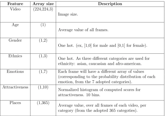
In this work we propose a multi-modal deep neural network which can be feeded with partial or all additional features previously described (age, gender, etc.). The only mandatory one, obviously, is the video stream, which constitutes the baseline for our experiments. Table 3.1 shows the array size, along with the description, of each extra feature.

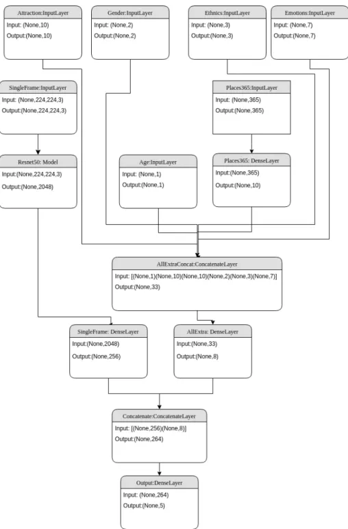
Figure 3.2 shows the complete architecture. Each extra information (video as only exception) is precomputed before hand. Detailed information and methodology used to extract additional features (emotion, attractiveness, etc) are provided in Section 3.3.

There is an important issue to consider regarding how to merge video information with the rest of the sources. There must be a clear balance between all of them, therefore the necessity of including some extra dense layers to adjust the sizes of the input arrays. Models with only one extra information source are simple. For instance, figure 3.3 shows the network architecture when only emotion information is included. The model with all the extra information sources minus background scene information has also the structure depicted in figure 3.2.

(32)

Feature Array size Description

Video (224,224,3)

Image size.

Age (1)

Average value of all frames. Gender (1,2)

One hot. (ex, [1,0] for male and [0,1] for female). Ethnics (1,3)

One hot. As three different categories are used for ethnicity: asian, caucasian and afro-american. Emotions (1,7) Each frame will have a different array of values

(corresponding to the probability distribution of each emotion, from the 7 adopted categories).

Attractiveness (1,10)

Normalized histogram of computed scores for attractiveness. 10 bins.

Places (1,365)

Average value, over all frames of each video, per category (from the adopted 365 categoties). Table 3.1: Information sources, size and description.

architecture we started with, was very similar to the final model. The main problem with this architecture is that in the concatenation layer, before the final 5 units dense layer, the sizes of the video stream and the rest of the features are too dissimilar (2048 for the video input vs no more than 10, for the rest of the features). This kind of difference made practically neglectable the influence of the extra information streams in compare with the video one.

The final solution was the one depicted in figure 3.2 because somehow balance the importance of different features in the right way, making a compact and highly accurate model.

3.2.2 Training the network

ResNet-50 was selected for image processing because is a state of the art, deep, architecture, which has proved to be useful in a wide range of problems.

(33)

3.2. Architecture 15

Figure 3.2: Full network architecture including all the extra information streams.

for apparent personality estimation. We define the baseline architecture as the one which only has video information.

Regarding the initial ResNet-50 weight values, Imagenet weights are loaded into the network.

The training is made in two steps. During the first stage we train only the new layers responsible to model the extra information, as well as the Dense layer related to the visual stream. The

(34)

Figure 3.3: Network architecture with only emotions information.

number of epochs is setted to 10 with a learning rate of 0.001. For the second stage, all layers are trained with a lower learning rate (0.0005) during 100 epochs. In order to improve the learning process, learning rate is automatically adjusted by a factor of 0.95 when no improvement was detected after 5 epochs. This mechanism is called reduce learning rate on plateau, and we use mean absolute error over validation dataset as metric to take the decision on when to reduce the learning rate.

Input size of the images is 224 by 224 pixels. Batch size is 25. Images shuffle procedure is not implemented. Initial weights for all the dense layers (ResNet-50 is preloaded with imagenet

(35)

3.3. Information sources 17

weights), are randomly selected from a glorot uniform distribution. In order to make the experiments reproducible, a fixed seed is used.

The final output layer has 5 units, one per each personality trait (extraversion, agreeableness, openness, conscientiousness, and neuroticism). The activation function of this layer is sigmoid, which is the standard activation function for regression problems. The loss function is mean square error (MSE) and the optimizer, is Adam with the following parameters: learning rate (as commented before, varies depending on training step), beta 1=0.9, beta 2=0.999, epsilon=1e-08, decay=0.0 and amsgrad flag setted to false.

Best models are constantly and automatically saved when improvement in the mean absolute error over the validation set is detected.

3.3 Information sources

3.3.1 Video stream

Due to limitations in computation resources (GPU) and time, only 10 frames for each video are extracted for training and validation and 50 frames per video for testing. The selected frames are equally distributed according to the video duration, assuring the presence of frames from all parts of the videos.

The number of frames equal to 10 was set based on experiments and represents a good balance between cost and benefit.

All the images are JPEG image data files, with density 1x1, segment length 16, precision 8, and resolution 1280x720. Image size is reduced to 224x224 (RGB), from its original size 1280x720.

(36)

3.3.2 Age

Age estimation is based on the work done by [RTVG15]. In that paper, a pretrained VGG network is adopted. However, the code we use to reproduce the results, adopt a Wide Residual Network (WideResNet) [ZK16] trained from scratch. Also, the original implementation of WideResNet was changed and two classification layers (for age and gender estimation) are added on the top of the WideResNet. Only age is considered because gender ground truth information was available in First Impressions dataset.

Age estimation needs only person face, therefore face detection is implemented as a first step. DLIB Frontal Face Detection [Kin09] is used for that task.

Age is estimated for all frames for all videos in the dataset. For some of the frames DLIB is not able to retrieve the face, therefore, age cannot be estimate. For the remaining frames, we compute the average of all the values, ending with a single age value for each video. This means that 10 images taken from the same video will have the same age value.

Figure 3.4: Age distribution IMDB + WIKI dataset [RTG16].

The authors of [RTVG15] used the IMDB-WIKI dataset to train the model. Which, at that time, was the largest publicly available dataset of face images with gender and age labels for training. It consist of a total of 460,723 face images from 20,284 celebrities from IMDb and

(37)

62,328 images from Wikipedia, thus 523,051 images in total [RTVG15]. Figure 3.4 shows age distribution for the IMDB + WIKI dataset.

Figure 3.5 shows some examples of age estimation for some videos of the First Impressions dataset.

Figure 3.5: Age estimation for some of the images for the First Impression dataset. From top to bottom, from left to right 34, 20, 19 and 21 years old respectively.

3.3.3 Gender

First Impressions dataset provides ground truth information regarding gender. A categorical variable called gender with values 1 for male and 2 for female is provided with this aim. One hot encoding is performed with this information, so a 2 values vector is the final size of the information source.

Gender can be automatically computed with state-of-the-art models [RTVG15]. We did not estimate gender values because automatic recognition of this attribute is not part of this master thesis.

(38)

3.3.4 Ethnics

The dataset also provides ground truth information about ethnics. In this regard, a categorical variable called ethnics is provided, with values 1 for Asian people, 2 for Caucasian and 3 for African-American. Again, one hot encoding is implemented, so finally a 3 values vector is the final size of this information source.

Also, ethnics can be automatically estimated [NB16]. Like gender, automatic estimation of this attribute is out of the scope of this master thesis.

3.3.5 Emotions

For emotion estimation we have used the code developed by Juan Luis Rosa, former student of the AI Master at the University of Barcelona, in his master thesis titled Deep Learning for Universal Emotion Recognition in Still images. The model is able to classify a face image into one of the following 7 classes: neutral, anger, disgust, fear, happy, sadness and surprise. The network used for emotion inference on our dataset is the Alexnet, which is the architecture finally proposed in his work.

The work presents several network architectures (AlexNet, VGG-16 and ResNet-50) trained with several datasets. Those dataset are the Japanese Female Facial Expression dataset [LAK+98], the Extended Cohn-Kanade dataset [LCK+10], the Karolinska Directed Emotional Face dataset [CL08], the Radboud Faces Database [LDB+10], the Oulu-CASIA dataset [ZHT+11] and many more.

First, as many others information sources, it is necessary to detect, extract and frontalize the faces from each frame all videos. DLIB is used with this purpose.

A key difference between this source and some of the others, is that here, no aggregation of the information is made for all the frame in a single video. In this case, for each frame we have a 7 value array probability distribution, each value ranging between [0,1] for each of the 6 emotions plus the neutral one.

(39)

An important issue to discuss, is that the author, found that for african-american, one the most predominant estimated emotion was anger, when it should have been neutral. This could in principle affect the performance of this information source for apparent personality estimation in african-american people.

Figure 3.6 show the most predominant estimated emotion for some of the frames in some videos of the First Impressions dataset.

Figure 3.6: Most predominant emotion for some images of the First Impressions dataset. From top to bottom, from left to right: sadness, disgust, neutral and fear respectively.

3.3.6 Attractiveness

The authors of [GYXG10] use a feed forward model to predict facial beauty, enabling the model to self detect facial features responsible for classifying beauty in faces. Prior models, like the one presented by [GT94] are based on face landmarks such as simmetry.

Estimation of attractiveness factor is made based on the work of [LLJ+_{18]. The authors tested}

three different architectures (AlexNet, ResNet-18 and ResNeXt-50) using the SCUT-FBP5500 dataset which was created by them.

(40)

including 2000 Asian females, 2000 Asian males, 750 Caucasian females and 750 Caucasian males. Figure 3.7 shows beauty scores [LLJ+_{18] for some images.}

Figure 3.7: Beauty scores examples from the paper [LLJ+_18].

In order to have an architecture capable of predicting the attractiveness factor, we have used the SCUT-FBP5500 dataset to train a modifided VGG16 model (i.e., the final layer was replaced by a dense layer of size=1, responsible to regress the attractive score). First of all, face extraction and frontalization is made using DLIB for each frame for all videos of the First Impressions dataset. Faces could not always be extracted from the videos because sometimes it was not detected. However we are able to apply this procedure to almost all the frames.

The original work ranked the attraction factor with values between 0 and 5. We modify it, with the objective of working with continuos values between 0 and 1. Imagenet weights are used as initial weights for the network. We have trained the network in two steps, first we trained only the last layer and later we fined tune all the layers.

As a result the output of the network will be a value ranging between [0,1] for each frame of the each video. So, in order to capture the richness of having diffent values of attractiveness for the same person in a video (due mainly to diffent face angles to the camera), we compute a normalized histogram from the scores obtained for all frames on each video using 10 bins. In this way, for each video, each frame has the same histogram of attractiveness.

(41)

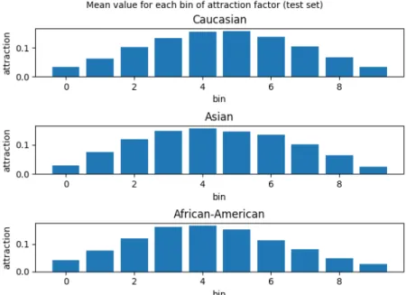
Figure 3.8: Average attractiveness factor histogram for the different populations according to ethnicity. First Impressions dataset.

SCUT-FBP5500 and First Impression datasets are very different. The first one, contains only caucasian and asian people faces, while the latter also has african-american faces. So, it could be expected, that the network has some problems when estimating the attraction score for african-american people. Fortunatly, this was not the case. Figure 3.8 shows the normalized histogram for the average attractiveness score of each of the three ethnics considered (caucasian, asian and african-american) on the First Impression dataset. While it is true that, the mean value of attractiveness seems to be higher for the caucassian population than for african-american population, the small diferences could not be considered as a true estimation bias.

3.3.7 Backgroud scene

With the aim of incorporating background scene information, code from [Pla] is used, which is based on the paper [ZLX+14].

Places365-Standard is a 1,803,460 training images dataset with the image number per class varying from 3,068 to 5,000. The validation set has 50 images per class and the test set has 900 images per class. From the original 434 classes, those with more than 4,000 images per class were selected, making a total of 365 classes. Places365-Challenge has extra 6.2 million images

(42)

along with all the images of Places365-Standard, making a total of roughly 8 million images, where at most 40,000 images per category. In 2018, an even larger version of the dataset was release ([ZLK+_18]).

Figure 3.9 shows prediction examples over randomly selected images of the Places365-Standard dataset.

Figure 3.9: Scene prediction results using the VGG16 for randomly selected images of the Places365-Standard dataset.

Several pre-trained CNN models are available for Places365-Standard: AlexNet-places365, GoogLeNet-places365, VGG16-places365, VGG16-hybrid1365, ResNet152-places365, which is a fine-tuned from ResNet152-ImageNet, ResNet152-places365, etc. We use the AlexNet archi-tecture because the code is publicly available.

Contrary to the good results with VGG16 for images of the Places365 dataset, figure 3.10 (bottom, right side) shows one frame of some of the videos of the First Impressions dataset. In all the cases, this methodology classifies with almost the same classes all the images. Therefore, no improvement of the results with respect to the baseline (only video stream) should be expected, given that no extra useful information is given to the network.

Perhaps this missclassification is due to the small variability of the background scene. A stronger reason, could be the fact that, the person occupies a big percentage of the image, therefore

(43)

Figure 3.10: Left: Probability vs CategoryClass (365 classes). Top Right: three most probable classes. Bottom Right: sample frame of sample video.

making harder to estimate the scene.

This feature will have a total of 365 values (probability distribution array), thus each value represents the probability for the scene to belong to a class.

As it will be shown in section 4, the inclusion of this particular feature did not improve the results. For this reason, the background information (as it was computed) is removed from the final model depicted in Figure 3.2.

(44)

Chapter 4 Results

This section includes a brief description of the hardware and software used for the experiments. It also presents the evaluation protocol used to validate the experiments. Later on, a description of experiments and discussion.

4.1 Implementation details and resources

All the experiments were run in a server at the Computer Vision Center at the Universit`at Aut´onoma de Barcelona. The server has 10 GPUs, 9 of the them are NVIDIA Geforce GTX 1080 with 12G of memory and the remaining one is a NVIDIA Quadro P6000 with 24 G of memory. We usually used one GPU per experiment and occasionally two, to speed up calculations.

The code was developed in Python, version 3.5.2. Tensorflow version 1.8.0 was used as backend and keras version 2.2.0 as a high level API to build, train and test the models.

Regarding extra python libraries, we used OpenCV version 3.4.1, Dlib version 19.13.1 and for graphics, Matplotlib version 3.0.1.

(45)

4.2. Evaluation protocol 27

4.2 Evaluation protocol

Equation 4.1 presents the way in which the accuracy is calculated. For each of the 5 big traits of personality (j ={1, ..,5}) a value of accuracy is calculated. Here pi,j is the predicted value for image i, for trait j; gti,j is the ground truth for image i, for trait j and N is the size of the test set. Both, predicted and ground truth values are continuous values ranging between 0 and 1. The maximum value the aacuracy can achieve is 1.

Accuracyj = 1− PN i=1 pi,j −gti,j N (4.1)

The evaluation protocol is the same as the one used in the ChalearnLAP First impression challenge [Chab]. However, one consideration should be made. The accuracy results will be very similar for all the experiments, which does not mean that the results are the same. Quite the contrary, a significant improvement of the predicted values of the personality traits, could derive in a small change in the overall accuracy value. This happens because the values of the scores are between 0 and 1, and for instance a 0.1 average difference between predicted and ground truth value, leads to an accuracy of 0.9.

With this in mind, besides presenting the overall accuracy results, we will show examples where the predicted values are closer to the ground truth, after the inclusion of extra information.

4.3 Experiments

Given the features described in table 3.1, we have performed several experiments by combining them, in order to get the best possible model with the architecture describe in section 3.2.

Let us first calculate how many experiments must be done to cover all the possibilities. Video stream is mandatory, because is the one that gives more information. The rest of the features are age, gender, ethnics, emotions, attractiveness and places (scene background information).

(46)

28 Chapter 4. Results

1. Taken in groups of one: 6 variables, taking 1 each time, and without repetitions, the exact number of combinations can be calculated with the following equation_{(6−1)!∗1!}6! = 6. So, the possible combinations are : {(Age), (Gender), (Ethnics), (Emotions), (Attractiveness), (Places)}.

2. Taken in groups of two: 6 variables, taking 2 each time, and without repetitions, the ex-act number of combinations can be calculated with the following equation _{(6−2)!∗2!}6! = 15. So, the possible combinations are : {(Age, Gender), (Age, Ethnics), (Age, Emotions), (Age, Attractiveness), (Age, Places), (Gender, Ethnics), (Gender, Emotions), (Gender, Attractiveness), (Gender, Places), (Ethnics, Emotions), (Ethnics, Attractiveness), (Eth-nics, Places), (Emotions, Attractiveness), (Emotions, Places), (Attractiveness, Places)}.

3. Taken in groups of three: 6 variables, taking 3 each time, and without repetitions, the exact number of combinations can be calculated with the following equation _{(6−3)!∗3!}6! = 20. So, the possible combinations are : {(Age, Gender, Ethnics), (Age, Gender, Emotions), (Age, Gender, Attractiveness), (Age, Gender, Places), (Age, Ethnics, Emotions), (Age, Ethnics, Attractiveness), (Age, Ethnics, Places), (Age, Emotions, Attractiveness), (Age, Emotions, Places), (Age, Attractiveness, Places), (Gender, Ethnics, Emotions), (Gender, Ethnics, Attractiveness), (Gender, Ethnics, Places), (Gender, Emotions, Attractiveness), (Gender, Emotions, Places), (Gender, Attractiveness, Places), (Ethnics, Emotions, At-tractiveness), (Ethnics, Emotions, Places), (Ethnics, Attractiveness, Places), (Emotions, Attractiveness, Places)}.

4. Taken in groups of four: 6 variables, taking 4 each time, and without repetitions, the exact number of combinations can be calculated with the following equation _{(6−4)!∗4!}6! = 15. So, the possible combinations are : {(Age, Gender, Ethnics, Emotions), (Age, Gender, Eth-nics, Attractiveness), (Age, Gender, EthEth-nics, Places), (Age, Gender, Emotions, Attrac-tiveness), (Age, Gender, Emotions, Places), (Age, Gender, Attractivenes, Places), (Age, Etnics, Emotions, Attractiveness), (Age, Etnics, Emotions, Places), (Age, Etnics, Attrac-tiveness, Places), (Age, Emotion, AttracAttrac-tiveness, Places), (Gender, Ethnics, Emotions, Attractiveness), (Gender, Ethnics, Emotions, Places), (Gender, Ethnics, Attractiveness,

(47)

4.3. Experiments 29

Places), (Gender, Emotions, Attractiveness, Places), (Ethnics, Emotions, Attractiveness, Places)}.

5. Taken in groups of five: 6 variables, taking 5 each time, and without repetitions, the exact number of combinations can be calculated with the following equation _{(6−5)!∗5!}6! = 6. So, the possible combinations are : {(Age, Gender, Ethnics, Emotions, Attractiveness), (Age, Gender, Ethnics, Emotions, Places), (Age, Gender, Ethnics, Attractiveness, Places), (Age, Gender, Emotions, Attractiveness, Places), (Age, Ethnics, Emotions, Attractive-ness, Places), (Gender, Ethnics, Emotions, AttractiveAttractive-ness, Places)}.

6. Taken in groups of six: 6 variables, taking 6 each time, and without repetitions, the exact number of combinations can be calculated with the following equation _{(6−6)!∗6!}6! = 1. So, the possible combinations are : {(Age, Gender, Ethnics, Emotions, Attractiveness, Places)}.

A total of 64 experiments, that could be done. Due to limitations in time and resources, only key relevant experiments have been done.

Id. V. A. G. Et. Em. At. P.

1 x 2 x x 3 x x 4 x x 5 x x 6 x x 7 x x 8 x x x x x x 9 x x x x x x x

Table 4.1: Experiments performed and which information stream was included in each one of them. V.(Video), A. (Age), G.(Gender), Et. (Ethnics), Em. (Emotions), At. (Attractiveness), P. (Places).

We decided to focus only in the very basic ones, with the objective of trying to catch how each of the extra information streams will behave in the final results. Table 4.1 shows the experiments presented in this master thesis. Experiment 8 (all of them minus background scene) is justified by the fact that, as we claimed before in the methodology section, background scene was poorly

(48)

calculated, mainly because the person is present in more than half of the image, making the scene detection, a very difficult task.

4.4 Discussion

This section analyse and discuss the experiments and results done in this study. Different anal-ysis are performed, such as single trait analanal-ysis (section 4.4.1), personality traits distribution discussion (section 4.4.2) and gender and ethnics discussion (section 4.4.4).

4.4.1 Single trait discussion

We begin this section by discussing how the addition of each information source influences each of the personality traits. Table 4.2 shows the accuracy values for each trait and each experiment. Figure 4.1 shows the same accuracy values in a much compact and visual way.

The first interesting behaviour, is that, for the extraversion trait, adding almost any of the features will end up in better accuracy results. The addition of solely background scene informa-tion did not improve overall results, and this can be correlated to the fact that this informainforma-tion stream is not contributing useful information, as it was stated in chapter 3, subsection 3.3.7. So from now we will not pay much atention to this information feature, mainly because, it will introduce noise to the system instead of actual information. The most oustanding results are achieved when all the features are included, and in particular when scene background is ignored.

Regarding theagreeablenesstrait, none of the extra information features improved the results when treated individually. Same as extraversion trait, the best model comes from experiment 8.

With respect to the third trait,conscientiousness, the accuracy values are much higher than for the rest of the traits, even only with baseline information. In this case, any of the extra

(49)

4.4. Discussion 31

Figure 4.1: Accuracy over test set. Each block of columns represent one experiment. Nine experiments are represented here, baseline, baseline + age, baseline + gender, baseline + eth-nics, baseline + emotions, baseline + attraction, baseline + places, baseline + all - places and baseline + all the features.

Id. V. A. G. Et. Em. At. P. E A C N O Avg.

1 x 0.907 0.908 0.916 0.905 0.908 0.909 2 x x 0.910 0.907 0.912 0.905 0.907 0.908 3 x x 0.910 0.906 0.915 0.905 0.906 0.908 4 x x 0.909 0.907 0.914 0.904 0.909 0.909 5 x x 0.911 0.907 0.915 0.906 0.909 0.910 6 x x 0.909 0.908 0.914 0.903 0.908 0.908 7 x x 0.908 0.907 0.913 0.904 0.908 0.908 8 x x x x x x 0.912 0.910 0.921 0.908 0.912 0.913 9 x x x x x x x 0.910 0.910 0.919 0.908 0.910 0.911

Table 4.2: Accuracy results over test set. Video (V.), age (A.), gender (G.), ethnics (Et.), emotions (Em.), attractiveness (At.) and places (P.). Personality traits: extraversion (E), agreeableness (A), conscientiousness (C), neuroticism (N) and openness (O).

information streams helped to improve accuracy performance when individually combined with the visual stream. The closest value to the baseline comes with the inclusion of emotions

(50)

in-32 Chapter 4. Results

formation, even though, the values are still low. We can conclude that conscientiousness trait estimation cannot be apparently improved by adding any of the information streams availables here, in an individual manner. Surprisingly, the accuracy for this trait was significantly im-proved when all features were integrated (even when considering scene background feature). Maybe the way all the extra features are combined is the key to improve conscientiousness trait.

For the fourth trait, neuroticism the accuracy values for each of the experiments are the lowest when comparing with the rest of the traits. The addition of emotions information have a positive efect in the estimation of this trait, by improving the accuracy values. And similary as before, the best result was obtained through the integration of all traits (case 8), either if places is considered or not.

For the last trait,openness, the accuracy results for the baseline and for the single extra source experiments are more or less the same, with the exception experiment 4 and 5. In these cases, when ethnics or emotions information is added, the accuracy value is improved. Again, the best model is the one with all the features minus background scene information. The accuracy value achieved by this model is far superior than the baseline. The integration of all extra information sources seems to be the key.

As it can be seen, the overall best improvement, disregarding the integration of all features, is obtained when emotion features have been included, suggesting that emotion expression have strong influence on apparent personality trait recognition.

The last column of each of the experiments depicted in figure 4.1 is the average accuracy value. Even though, we consider that the right way to proceed is to analyze each trait in a separate way, by averaging the acurracy values for all the traits, we have a methodology to evaluate how good is the addition of a particular information source, for the problem of apparent personality estimation, using the OCEAN model.

The best model is the one from experiment 8. With an average accuracy over the test set of 0.913.

(51)

4.4. Discussion 33

4.4.2 Personality traits distribution discussion

In this section we discuss and analyse how the scores for each attribute are distributed. Figures 4.2, 4.3, 4.4, 4.5, 4.6 and 4.7 present the distribution of the scores for ground truth, baseline and experiments 2, 3, 4, 5, 6 and 7 respectively. The idea behind this section is to described in a global manner estimated personality trait scores vs ground truth.

Figure 4.2: Personality trait score histogram for each of the five traits (extraversion, agree-ableness, openness, conscientiousness and neuroticism). Ground truth, baseline and baseline + age.

In case of baseline plusage, the distribution curve for almost all of the traits looks very similar to the baseline distribution, suggesting that the inclusion of age, individually, have almost no effect on the results when compared to the baseline. For almost all traits, with the exception of conscientiousness, the ground truth has a wider distribution of values, in comparison with the estimated values, which concentrates more around the mean. This is a constant in all experiments, although for some of them, the obtained distribution get very close to the ground truth. The fact that the ground truth distribution of conscientiousness trait is very similar to the experiment distribution could be a way to understand why the accuracy values for this trait are higher than every other, for all the experiments.

(52)

Figure 4.3 shows the effect on the distribution when gender is included. The effect of this information source does not seem to make much improvement to the distribution, more over, as figure 4.1 shows, the only benefit of incorporating this information, is an improvement on the extraversion trait estimation.

Figure 4.3: Personality trait score histogram for each of the five traits (extraversion, agree-ableness, openness, conscientiousness and neuroticism). Ground truth, baseline and baseline + gender.

Table 4.2 shows how the addition of ethnicsimproves the estimation of extraversion, neuroti-cism and openness. This behaviour can be seen in the distribution curves of these three traits (figure 4.4). In all cases, the addition of ethnicity makes wider the distribution of the scores for these traits. Definetly, ethnics information, should be taken as one of the main information sources considered.

The most interesting case is the addition of emotions information. Figure 4.5 shows the score distribution for ground truth, baseline and baseline with emotions. With respect to the previous information sources, the addition of emotion information, clearly modifies in a significant manner the distribution of the scores. This effect can be perceived in all the traits with the exception of conscientiousness. This trait again, seems to remain more or less constant

(53)

4.4. Discussion 35

Figure 4.4: Personality trait score histogram for each of the five traits (extraversion, agree-ableness, openness, conscientiousness and neuroticism). Ground truth, baseline and baseline + ethnics.

regarding the addition of individual information sources.

With respect to the addition of attractiveness factor, the score distribution depicted in figure 4.6, shows very small improvement in the curve distribution, with the possible exception of extraversion trait, which always showed itself as very favorable to newly information sources. Even thought we said scene background information is not a useful source of information, due to the errors during the classification process, mainly because a person is occuping almost all the scene; we end this section by commenting how the addition of this source changes the distribution curve of the baseline. Figure 4.7 shows the distribution curve when this feature is included. Here the addition of background scene information is making the distribution more concentrated than before, instead of making it wider.

We think this effect is because, given the scene estimation is more or less the same for all the images in the dataset, when we feed the architecture with this information, is like saying that all the images are the same, and therefore, a concentrated distribution should be expected.

(54)

Figure 4.5: Personality trait score histogram for each of the five traits (extraversion, agree-ableness, openness, conscientiousness and neuroticism). Ground truth, baseline and baseline + emotions.

Figure 4.6: Personality trait score histogram for each of the five traits (extraversion, agree-ableness, openness, conscientiousness and neuroticism). Ground truth, baseline and baseline + attraction factor.

(55)

4.4. Discussion 37

Figure 4.7: Personality trait score histogram for each of the five traits (extraversion, agree-ableness, openness, conscientiousness and neuroticism). Ground truth, baseline and baseline + places.

4.4.3 Estimation improvements examples

This section shows some qualitative results achieved when adding each of the information sources. In all cases, what we present here are images from the top 20 best results where the model with the extra information source is superior to the baseline model. Score values for the ground truth, the baseline and the baseline plus the extra information source are reported for quantitative comparison.

The examples show in the next figures are for those trait / experiments combinations, where the extra information addition leads to better overall results.

Figure 4.8 shows the scores for 4 images for extraversion trait when age information is included. As can be seen, images in the top 20 best results, belong to caucasian females.

(56)

Figure 4.8: Images of videos from the top 20 most accurate image results (extraversion). Base-line (B) vs Improve model (age). Ground truth (GT). 1) GT:0.85046726, B:0.4894714, B+A: 0.78445417; 2) GT:0.3364486, B:0.6353641, B+A: 0.37536004; 3) GT:0.69158876, B:0.43417218, B+A: 0.6644097; 4) GT:0.76635516, B:0.52502894, B+A: 0.75191694.

Figure 4.9 shows the scores for extraversion trait with video plus gender information. Again, caucasian female in the top 20. Image number 2 has one of the best performances in experiments 2, 3 and 4. Image 1 and 2 belong to the best performant videos for extraversion (experiment 3).

Figure 4.9: Images of videos from the top 20 most accurate image results (extraversion). Base-line (B) vs Improve model (gender). Ground truth (GT). 1) GT:0.6635514, B:0.3455922, B+G: 0.65422666; 2) GT:0.85046726, B:0.4894714, B+G: 0.7789629.

Figure 4.10 shows the scores for extraversion trait when ethnics information is added. Mostly female in top 20 and only two caucasian males (only one is shown).

(57)

4.4. Discussion 39

Figure 4.10: Images of videos from the top 20 most accurate image results (extraversion). Baseline (B) vs Improve model (ethnics). Ground truth (GT). 1) GT:0.85046726, B:0.5119484, B+ET: 0.750787; 2) GT:0.7570093, B:0.5042182, B+ET: 0.726135; 3) GT:0.6635514, B:0.3894887, B+ET: 0.608043; 4) GT:0.5794392, B:0.3630559, B+ET: 0.57859546.

Figure 4.11 shows the scores when ethnics information is added for neuroticism trait. Frame 1 and 2 belong to the same video, which has the best accuracy results for neuroticism.

Figure 4.11: Images of videos from the top 20 most accurate image results (neuroticism). Baseline (B) vs Improve model (ethnics). Ground truth (GT). 1) GT:0.73333335, B:0.37926748, B+ET: 0.67457247; 2) GT:0.73333335, B:0.39857784, B+ET: 0.6830916.

The last two figures present frames of the top performant with emotions information. Figure 4.12 shows the scores for conscientiousness. Image 2 is present also figure figure 4.13 (neuroti-cism). Again, videos with caucasian females achieve the most accurate results.

(58)

Figure 4.12: Images of videos from the top 20 most accurate image results (conscientiousness). Baseline (B) vs Improve model (emotions). Ground truth (GT). 1) GT:0.34375, B:0.6799654, B+EM: 0.4277872; 2) GT:0.8645833, B:0.3954034, B+EM: 0.6284485; 3) GT:0.8333333, B:0.55324715, B+EM: 0.77577513; 4) GT:0.36458334, B:0.6222483, B+EM: 0.4058559.

Figure 4.13: Images of videos from the top 20 most accurate image results (neuroticism). Base-line (B) vs Improve model (emotions). Ground truth (GT). 1) GT:0.43333334, B:0.6767487, B+EM: 0.44482204; 2) GT:0.7777778, B:0.52615035, B+EM: 0.7380421.

We performed this analysis in the hope of finding some visual key pattern or some feature, that give us a clue of why the scores are much closer to the ground truth, when including the extra information source. Sadly, we cannnot extract any conclusion on the matter.

Finally and probably the most important feature that can be extracted is the fact that a great percentage of the better estimated videos are from caucasian female people. We can think that the addition of information of age, gender, ethnicity, emotions and facial beauty could help to estimate personality traits far better for female than for men. With this regard, subsection 4.4.4 analyse the accuracy segmented by gender and ethnics.

(59)

4.4. Discussion 41

4.4.4 Gender and Ethnics discussion

With the idea of corroborate if the model estimates are better for female than for men, we decide to analize the accuracy for some experiment for the following population segments: asian male, caucasian male, african-american male, asian female, caucasian female and african-american female. The experiments conducted only include age, emotions or attractiveness factor. Table 4.3 shows the number of images per segment in the test set.

Asian Caucasian African-American

Male 700 40200 3500

Female 1700 46200 7700

Table 4.3: Total number of images for test set for the following population segments: Male-Asian, Male-Caucasian, Male-AfricanAmerican, Male-Asian, Caucasian and Female-AfricanAmerican.

Figure 4.14 shows personality traits accuracy results in test set, for all population segments considered with age information. Accuracy results for females for all the ethnics are higher than for males.

Figure 4.14: Personality trait accuracy by population segment. (As: Male-Asian, Ma-Ca: Male-Caucasian, Ma-Af: Male-AfricanAmerican, Fe-As: Asian, Fe-Ma-Ca: Female-Caucasian and Fe-Af: Female-AfricanAmerican) with age information.

Multiple attribute analysis for deep learning based apparent personality analysis

Universitat Polit`ecnica de Catalunya

Facultat d’Inform`

atica de Barcelona

Multiple attribute analysis for deep learning

based apparent personality analysis

Ricardo Dar´ıo P´erez Principi

Abstract

Acknowledgements

Dedication

Contents

List of Tables

List of Figures

Chapter 1

Introduction

1.1

Motivation and Objectives

1.2

Contributions

1.3

Statement of Originality

Chapter 2

Background Theory

2.1

Previous work

2.2

Big Five Personality Model

2.2.1

Openness

2.2.2

Conscientiousness

2.2.3

Extraversion

2.2.4

Agreeableness

2.2.5

Neuroticism

2.3

ChaLearn Challenge

Chapter 3

Methodology

3.1

Dataset

3.2

Architecture

3.2.1

Full and partial architecture

3.2.2

Training the network

3.3

Information sources

3.3.1

Video stream

3.3.2

Age

3.3.3

Gender

3.3.4

Ethnics

3.3.5

Emotions

3.3.6

Attractiveness

3.3.7

Backgroud scene

Chapter 4

Results

4.1

Implementation details and resources

4.2

Evaluation protocol

4.3

Experiments

4.4

Discussion

4.4.1

Single trait discussion

4.4.2

Personality traits distribution discussion

4.4.3