Case Studies of a Machine Learning Process for Improving the Accuracy of Static Analysis Tools

(1)

Case Studies of a Machine Learning

Process for Improving the Accuracy

of Static Analysis Tools

by

Peng Zhao

A thesis

presented to the University of Waterloo in fulfillment of the

thesis requirement for the degree of Master of Mathematics

in

Computer Science

Waterloo, Ontario, Canada, 2016

c

(2)

I hereby declare that I am the sole author of this thesis. This is a true copy of the thesis, including any required final revisions, as accepted by my examiners.

(3)

Abstract

Static analysis tools analyze source code and report suspected problems as warnings to the user. The use of these tools is a key feature of most modern software development processes; however, the tools tend to generate large result sets that can be hard to process and prioritize in an automated way. Two particular problems are (a) a high false positive rate, where warnings are generated for code that is not problematic and (b) a high rate of non-actionable true positives, where the warnings are not acted on or do not represent significant risks to the quality of the source code as perceived by the developers. Previous work has explored the use of machine learning to build models that can predict legiti-mate warnings with logistic regression [38] against Google Java codebase. Heckman [19] experimented with 15 machine learning algorithms on two open source projects to classify actionable static analysis alerts.

In our work, we seek to replicate these ideas on different target systems, using different static analysis tools along with more machine learning techniques, and with an emphasis on security-related warnings. Our experiments indicate that these models can achieve high accuracy in actionable warning classification. We found that in most cases, our models outperform those of Heckman [19].

(4)

Acknowledgements

First, I would like to extend my sincere gratitude to my supervisor, Michael Godfrey, for his helpful guidance on my thesis.

I am deeply grateful for Andrew Walenstein, Andrew Malton, and Jong Park for their great help and useful suggestions to my thesis.

(5)

Dedication

(6)

List of Tables

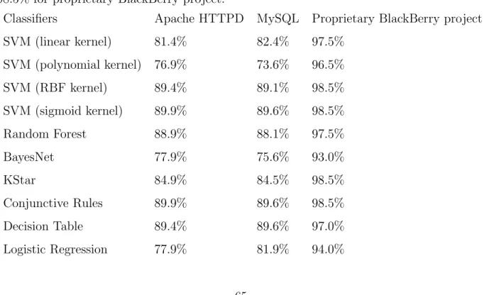
1.1 Three Research Questions and Methods of the thesis . . . 8 4.1 Names and explanations of all the features extracted in our project . . . . 25 6.1 Accuracy of highest results of classifiers on Apache HTTPD, MySQL, and

Proprietary BlackBerry project . . . 37 6.2 Correlated precision of highest accuracy of best classifiers on Apache HTTPD,

MySQL, and proprietary BlackBerry project . . . 38 6.3 Correlated recall of highest accuracy of best classifiers on Apache HTTPD,

MySQL, and proprietary BlackBerry project . . . 38 6.4 Features that have ever been selected for all three projects with seven feature

selection strategies. . . 42 6.5 Accuracy of highest results of feature selection strategies on Apache HTTPD,

MySQL, and proprietary BlackBerry project . . . 44 6.6 Correlated precision of highest accuracy of best feature selection strategies

on Apache HTTPD, MySQL, and proprietary BlackBerry project . . . 45 6.7 Correlated recall of highest accuracy of best feature selection strategies on

Apache HTTPD, MySQL, and proprietary BlackBerry project . . . 46 6.8 Accuracy of the highest results of resampling techniques for Apache HTTPD,

MySQL, and proprietary BlackBerry project.. . . 47 6.9 Correlated precision of the highest accuracy of resampling techniques for

Apache HTTPD, MySQL, and proprietary BlackBerry project. . . 48 6.10 Correlated recall of the highest accuracy of resampling techniques for Apache

(10)

6.11 Accuracy of the highest results of cost-sensitive techniques for Apache HTTPD, MySQL, and proprietary BlackBerry project.. . . 49 6.12 Correlated precision of the highest accuracy of cost-sensitive techniques for

Apache HTTPD, MySQL, and proprietary BlackBerry project. . . 50 6.13 Correlated recall of the highest accuracy of cost-sensitive techniques for

Apache HTTPD, MySQL, and proprietary BlackBerry project. . . 51 6.14 Accuracy of the highest results of Heckman’s methodology on our dataset. 53 6.15 Correlated precision of highest accuracy of Heckman’s methodology on our

dataset. . . 54 6.16 Correlated recall of highest accuracy of Heckman’s methodology on our

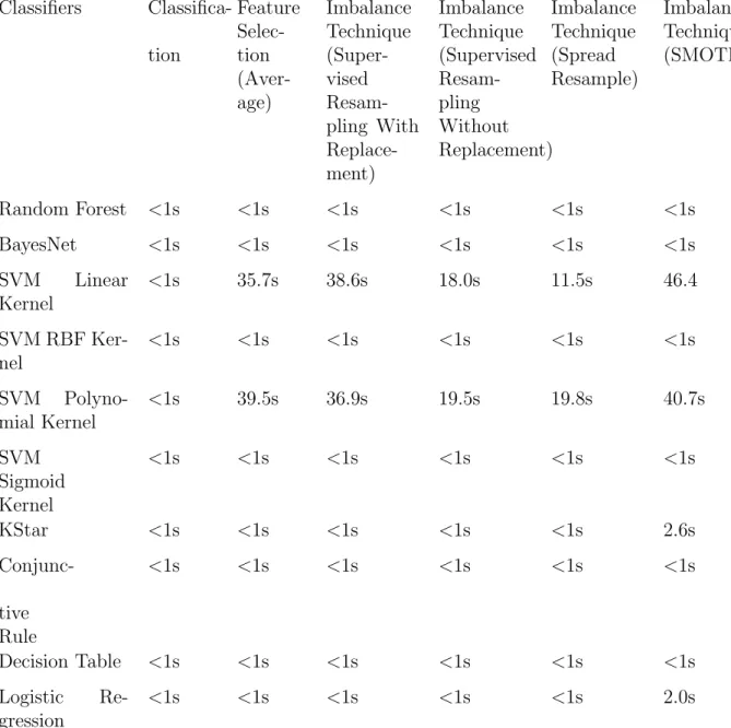
dataset. . . 55 6.17 Execution time in classification, average time for one process in feature

selection and resampling imbalance techniques for MySQL datasets. . . 56 6.18 Execution time in cost sensitive imbalance techniques for MySQL datasets. 57 A.1 All the accuracies of actionable warnings classification on three projects with

classifiers. . . 65 A.2 All the precisions of actionable warnings classification on three projects with

classifiers. . . 66 A.3 All the recalls of actionable warnings classification on three projects with

classifiers. . . 67 A.4 All the accuracies of actionable warnings classification on Apache HTTPD

with combinations of seven feature selection strategies and seven classifiers 68 A.5 All the precisions of actionable warnings classification on Apache HTTPD

with combinations of seven feature selection strategies and seven classifiers. 69 A.6 All the recalls of actionable warnings classification on Apache HTTPD with

combinations of seven feature selection strategies and seven classifiers. . . . 70 A.7 All the accuracies of actionable warnings classification on MySQL with

com-binations of seven feature selection strategies and seven classifiers. . . 71 A.8 All the precisions of actionable warnings classification on MySQL with

(11)

A.9 All the recalls of actionable warnings classification on MySQL with combi-nations of seven feature selection strategies and seven classifiers . . . 73 A.10 All the accuracies of actionable warnings classification on proprietary

Black-Berry project with combinations of seven feature selection strategies and seven classifiers. . . 74 A.11 All the precisions of actionable warnings classification on proprietary

Black-Berry project with combinations of seven feature selection strategies and seven classifiers. . . 75 A.12 All the recalls of actionable warnings classification on proprietary

Black-Berry project with combinations of seven feature selection strategies and seven classifiers. . . 76 A.13 All the accuracies of actionable warnings classification on Apache HTTPD

project with resampling techniques. All the classifiers are trained with the reconstructed datasets generated by resampling techniques. KStar and su-pervised resampling with replacement achieve the highest accuracy at 93.5%. 77 A.14 All the precisions of actionable warnings classification on Apache HTTPD

project with resampling techniques. All the classifiers are trained with the reconstructed datasets generated by resampling techniques. Decision Table and spread subsample achieve the highest precision at 100.0%. . . 78 A.15 All the recalls of actionable warnings classification on Apache HTTPD project

with resampling techniques. All the classifiers are trained with the recon-structed datasets generated by resampling techniques. A few classifiers such as SVM Sigmoid Kernel with supervised resampling with replacement achieve 100.0% recall. . . 79 A.16 All the accuracies of actionable warnings classification on MySQL project

with resampling techniques. All the classifiers are trained with the recon-structed datasets generated by resampling techniques. The highest accuracy is achieved by Logistic Regression and supervised resampling replacement. 80 A.17 All the precisions of actionable warnings classification on MySQL project

with resampling techniques. All the classifiers are trained with the recon-structed datasets generated by resampling techniques. The highest precision is achieved by Logistic Regression and supervised resampling with replacement 81

(12)

A.18 All the recalls of actionable warnings classification on MySQL project with resampling techniques. All the classifiers are trained with the reconstructed datasets generated by resampling techniques. Supervised resampling with replacement and KStar achieve 100.0% recall. . . 82 A.19 All the accuracies of actionable warnings classification on proprietary

Black-Berry project with resampling techniques. All the classifiers are trained with the reconstructed datasets generated by resampling techniques. A few clas-sifiers with supervised resampling with replacement achieve 100.0% accuracy. 83 A.20 All the precisions of actionable warnings classification on proprietary

Black-Berry project with resampling techniques. All the classifiers are trained with the reconstructed datasets generated by resampling techniques. A few clas-sifiers with supervised resampling with replacement achieve 100.0% precision. 84 A.21 All the recalls of actionable warnings classification on proprietary

Black-Berry project with resampling techniques. All the classifiers are trained with the reconstructed datasets generated by resampling techniques. All the classifiers with supervised resampling with replacement achieve 100.0% recall. . . 85 A.22 All the accuracies of actionable warnings classification on Apache HTTPD

project with cost-sensitive techniques. SVM RBF Kernel and cost-sensitive prediction achieves highest accuracy at 91.5%. . . 86 A.23 All the precisions of actionable warnings classification on Apache HTTPD

project with cost-sensitive techniques. The highest precision is achieved by SVM RBF Kernel and cost-sensitive prediction. . . 87 A.24 All the recalls of actionable warnings classification on Apache HTTPD project

with cost-sensitive techniques. The highest recall is achieved by Conjunctive Rules with cost-sensitive prediction. . . 88 A.25 All the accuracies of actionable warnings classification on MySQL project

with cost-sensitive techniques. The best classifier is SVM which achieves 89.1% accuracy with cost-sensitive prediction. . . 89 A.26 All the precisions of actionable warnings classification on MySQL project

with cost-sensitive techniques. Most of the precisions for MySQL despite of classifiers are from 10.0% to 20.0% . . . 90 A.27 All the recalls of actionable warnings classification on MySQL project with

cost-sensitive techniques. Conjunctive Rules and Decision Table both achieve 100.0% recall with cost-sensitive prediction. . . 91

(13)

A.28 All the accuracies of actionable warnings classification on proprietary Black-Berry project with cost-sensitive techniques. All the accuracies are over 90.0% except from classifier BayesNet despite of cost-sensitive techniques. . 92 A.29 All the precisions of actionable warnings classification on proprietary

Black-Berry project with cost-sensitive techniques. The highest precision is achieved by KStar and meta-cost at 50.0%. . . 93 A.30 All the recalls of actionable warnings classification on proprietary

Black-Berry project with cost-sensitive techniques. The highest recall achieved by a few classifiers is 66.7%. . . 94

(14)

List of Figures

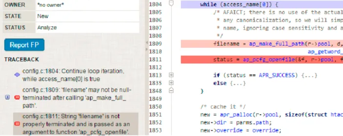
1.1 A non-actionable warning example from Apache HTTPD. In the example, the return value from functionap make full path is not properly termi-nated. . . 4 4.1 Process of feature extraction, feature selection, ground truth labeling, and

machine learning in Prioritizer . . . 21 4.2 An example of a warning that labeled as actionable from CSAT analysis of

MySQL . . . 27 4.3 The fix of the actionable labeled warning from CSAT analysis of MySQL . 27 4.4 An example of a warning that labeled as non-actionable from CSAT analysis

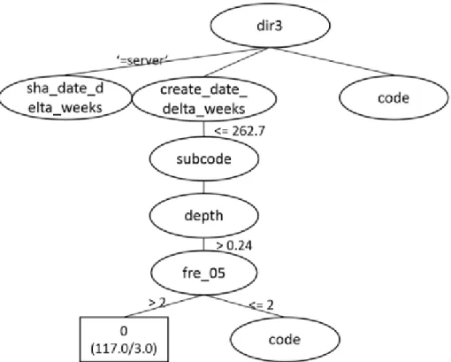
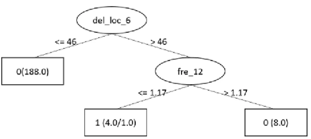
of MySQL . . . 28 6.1 Random Forest trained on Apache HTTPD dataset to classify actionable

warnings(partial) . . . 39 6.2 Random Forest trained on MySQL dataset to classify actionable

warn-ings(partial) . . . 40 6.3 Random Forest trained on proprietary BlackBerry project to classify

(15)

Chapter 1 Introduction

Large computer systems invariably have bugs. To combat this problem, many kinds of tools have been designed to analyze software systems in different ways. One class of these tools, known asstatic analyzers or static analysis tools, analyze programs by examining the source code, such as looking for poor programming style and known bad designs, extracting dependency information about program entities such as control flow graphs, and building various kinds of models of the structure of the program source code. These tools are called static because they perform their tasks without actually executing the system. Findbugs is an open source example of a static analyzer for Java that is in wide use.

Many companies employ static analysis tools as part of their development process; they may use them for a variety of purposes, such as performing quality assurance or as part of a code review process. In particular, systems that require unusually strong assurance of reliability and trust may use static analysis tools to look for critical bugs and detect known security vulnerabilities. For example, in our studies we have used a commercial tool which we shall refer to as CSAT (Commercial Static Analysis Tool); used by development teams that work on high-security systems, this tool pays special attention to well-known classes of security vulnerabilities, such as the Common Weakness Enumeration database (CWE). 1 Performing a myriad of checks for well-known problems such asBuffer Overflow,Injection,

and Null Pointers Dereferencing, CSAT also allows developers to add their own checks to

their CSAT installation. For example, Blackberry adds dozens of their own checkers to look out for specific security concerns in their systems.

One of the major problems of existing static analysis tools is the amount of non-automatable work that it takes to get useful results. By their nature, static analysis 1_{A non-disclosure agreement with our industrial partner prevents us from identifying CSAT by name.}

(16)

tools have only an imperfect idea of the meaning of the underlying code; they tend to assume that all possible problems should be reported, resulting in a high false-positive rate. Furthermore, it is known that off-the-shelf static analysis tools often report perceived problems that developers may not consider worth acting on. For example, in Google [38],

for Findbugs, only 55% of the warnings are addressed after loging into a bug tracking

system. Thus, even if a reported problem is a true-positive, it may not be considered to

be actionable by the development team. In BlackBerry, fewer than 10% of the warnings

from CSAT were acted on by engineers.

Listing 1.1 shows an actionable warning example of demonstration from CSAT that detected in Apache HTTPD 2.2.10. The fix of the warning (bug) in Apache HTTPD 2.2.16 is shown in Listing 1.2.

1 char kb[MAX_STRING_LEN];

2 int i = 0;

3 rv = apr_dbm_firstkey(htdbm->dbm, &key);

4 if (rv != APR_SUCCESS) {

5 fprintf(stderr, "Empty database -- %s\n", htdbm-> ,→ filename);

6 return APR_ENOENT;

7 }

8 while (key.dptr != NULL) {

9 rv = apr_dbm_fetch(htdbm->dbm, key, &val);

11 fprintf(stderr, "Failed getting data from %s\n",

,→ htdbm->filename);

12 return APR_EGENERAL;

13 }

14 strncpy(kb, key.dptr, key.dsize);

15 kb[key.dsize] = ’\0’;

16 fprintf(stderr, " %-32s", kb);

Listing 1.1: An actionable warning that CSAT detected in Apache HTTPD 2.2.10 usage of unsafe String API “strncpy”

The checker that caused the warning is looking for occurences of the C library function

strncpy which is historically unreliable and not a best practice according to security experts. The function copies a certain number of characters from source to destination. It

(17)

does not require a terminator at the end of the destination string so it could be susceptible to a variety of exploits such as buffer overflow.

In this case,strncpy copieskey.dptr tokbwith the length of key.dsize. Then \0-terminator is added to the end of kb before printing kb out. If key.dsize>=

MAX STRING LEN then there is a buffer overflow in kb. avoid using kb, so there won’t have buffer overflow In Listing1.2,printfprints out characters fromkey.dptrdirectly without using dbwhich avoids buffer overflow.

1 while (key.dptr != NULL) {

2 rv = apr_dbm_fetch(htdbm->dbm, key, &val);

4 fprintf(stderr, "Failed getting data from %s\n",

,→ htdbm->filename);

5 return APR_EGENERAL;

6 }

7 /* Note: we don’t store \0-terminators on our dbm data ,→ */

8 fprintf(stderr, " %-32.*s", (int)key.dsize, key.dptr

,→ );

9 cmnt = memchr(val.dptr, ’:’, val.dsize);

10 if (cmnt)

11 fprintf(stderr, " %.*s", (int)(val.dptr+val.dsize

-,→ (cmnt+1)), cmnt + 1);

12 fprintf(stderr, "\n");

Listing 1.2: Fix of the example of the actionable warning in Apache HTTPD 2.2.16 that removed the usage of String APIstrncpy

A non-actionable warning example in Figure 1.1 refers to the return value filename from the function ap make full path. The return value filename is not terminated properly. The comments of the function is shown in Listing 1.3 and the code of the function ap make full path is shown in Listing 1.4.

(18)

Figure 1.1: A non-actionable warning example from Apache HTTPD. In the example, the return value from function ap make full path is not properly terminated.

1 /*

2 _{* @return A copy of the full path, with one byte of extra} ,→ space after the NUL

3 _* to allow the caller to add a trailing ’/’.

4 _{* @note Never consider using this function if you are dealing} ,→ with filesystem

5 _{* names that need to remain canonical, unless you are merging} ,→ an apr_dir_read

6 _{* path and returned filename.} Otherwise, the result is not ,→ canonical.

7 _*/

8 AP_DECLARE(char _{*) ap_make_full_path(apr_pool_t *a,} const char

,→ *dir, const char *f)

9 AP_FN_ATTR_NONNULL_ALL;

Listing 1.3: Comment of the function ap make full path that caused problems in the non-actionable warning example

1 AP_DECLARE(char _{*) ap_make_full_path(apr_pool_t *a,} const char

,→ *src1,

(19)

3 {

4 apr_size_t len1, len2;

5 char _*path;

6

7 len1 = strlen(src1);

8 len2 = strlen(src2);

9 /* allocate +3 for ’/’ delimiter, trailing NULL and ,→ overallocate

10 _{* one extra byte to allow the caller to add a trailing} ,→ ’/’

11 _*/

12 path = (char _{*)apr_palloc(a, len}1 + len2 + 3);

13 if (len1 == 0) { 14 _{*path =} ’/’; 15 memcpy(path + 1, src2, len2 + 1); 16 } 17 else { 18 char _*next; 19 memcpy(path, src1, len1);

20 next = path + len1;

21 if (next[-1] != ’/’) { 22 _{*next++ =} ’/’; 23 } 24 memcpy(next, src2, len2 + 1); 25 } 26 return path; 27 }

Listing 1.4: Code in the functionap make full path that generated the non-actionable warning example

The code and comment of the functionap make full path verify the imperfect de-sign of leaving one byte of extra space at the end of the return value. However, this warning has never been fixed in their later versions of the code, presumably because the developers did not consider it to be a serious risk. As long as a warning has never been acted on, we define the warning as non-actionable.

(20)

reduce the rate of non-actionable true-positives of static analysis tools for both industrial and open source projects. We build on previous work by Ruthruff [38] and Heckman [19]. Ruthruff adopted logistic regression on highly associated features against Google’s Java codebase, while Heckman enlarged the feature sets from Ruthruff and compared more popular machine learning models with selected features on open source Java projects.

Different from previous work, we explore the static analysis tool CSAT with a security focus on both open source and commercial projects. We improve the usability and value of static analysis tool by classifying actionable warnings. Ordinarily, static analysis tools neither classify nor filter their output. Our Prioritizer project serves to develop techniques to automatically classify as “actionable” and “non-actionable” warnings using machine learning models. These machine learning models are derived from training the models on labeled warnings generated by static analysis tools. One novel contribution of our work is the security focus during the analyses which causes more false positives. A second contribution of this project is the usage of machine learning techniques to handle the extremely high ratio of false positives. A third innovative aspect concerns the generation of the datasets, which consist of features and associated metrics that are extracted from the source code repository and the development context. Features and associated metrics are properties of source code repositories, source code development histories, static analysis tool settings, and static analysis tool warnings histories. Significantly, the code repository, development context, and static analysis tool warnings histories are typically not exploited by static analysis tools. However, the context information shows statistical significance in machine learning models. Some features are strongly correlated with the actionability of warnings. We expect the results of our research to increase the usability of static analysis tools for both open-source and commercial projects by using code contexts information.

Security experts at Blackberry, our industrial collaborator on this project, have selected a set of default settings for the use of CSAT; in part, this is based on CSAT’s off-the-shelf default settings. Apart from this set of default settings, security experts added customized BlackBerry security checkers. The regular setting of CSAT enables its critical checkers to detect potential critical bugs in less than an hour for Apache HTTPD. Those customized BlackBerry security checkers cover a variety of known issues, such as the uses of unsafe string API, misuse of memcpy, and customized message handlers.

The goal of this research is to improve the accuracy of static analysis tools with a secu-rity focus related to actionability. We use supervised machine learning models and feature selection algorithms on source code and extra-code (“context”) features. The security em-phasis, supervised machine learning techniques for imbalanced datasets, and commercial static analysis tools distinguish our work from previous work. We propose a portable pro-cess of building machine learning models with features extracted from customized CSAT

(21)

analysis and experiment with different projects in the following steps: 1) analyze different versions of source code; 2) extract features and explore strongly correlated feature sets; and 3) compare different classifiers with highly imbalanced datasets including classifica-tion, feature selecclassifica-tion, and imbalance handling. We conduct experiments and validation on both commercial and open-source projects.

We found that thousands of warnings are generated by our use of CSAT using the target systems of Apache HTTPD, MySQL, and BlackBerry code base. Sampling hundreds of warnings from them, our models classify actionable warnings. In our experiments, models trained with the oversampling datasets correctly classify 90% of the warnings from the datasets according to their actionability. These models achieve 100% recall, which means these models classify all the actionable warnings as actionable. Our experiments improve CSAT performance within BlackBerry and also indicate a method of improving security vulnerability detection.

1.1 Problem

Static analysis tools detect potential critical bugs and generate warnings without ex-ecuting the code. There are three risks in detecting actionable warnings. First, static analysis tools detect a restricted number of (actionable) warnings but involve two trade offs: false negatives versus false positives and accuracy vesus efficiency. This often results in high false positive rates. Simultaneously, the static analysis tool provides flexibility for users to adjust tradeoffs. It is historically difficult for users to successfully adjust the sensitivity without a fair amount of experimentation. Second, the tools normally output all the generated warnings without any filter or classification. With a high false positive rate, most of the warnings displayed by static analysis tools are not useful for developers. Third, the tools are typically not written to consider reporting warnings based on non-program factors, such as frequency of code update, project type, and project sensitivity, each of which has a significant value in actionable warnings prediction. However, those non-program factors are not included in the scope of most static analysis tools.

1.2 Research Questions

With the problems we came across, table 1.1 lists the research questions that are in scope for this research, and states the approach we will use.

(22)

Research Question Research Method RQ1 What features are useful for predicting

security vulnerability warnings?

Over-generate features that arguably are correlated to vulnerabilities and use feature selection measures and accu-racy observed to rank, evaluate, and se-lect.

RQ2 What statistical models best predict actionable warnings?

Explore supervised machine learning algorithms and analyze their execution time

RQ3 What are the differences between com-mercial and open-source projects?

Compare commencial and open-source projects with same techniques

Table 1.1: Three Research Questions and Methods of the thesis

1.3 Contributions

There are three main research contributions of this work:

1. A method for generating a predictive statistical model for filtering actionable static analysis tool warnings that improves upon prior work in terms of accuracy and utilizes features not explored in prior research.

2. An analysis of the utility of an extensive set of code and non-code features are predictive of actionability of static analysis tool warnings. This includes measuring and characterizing the utility of introduced features as well as previously used ones (which were never evaluated in this way).

3. A method for selecting classifiers and machine learning techniques for predicting actionable warnings from static analysis tools by combining rule-based (expert) filters with the statistical classifier.

1.4 Organization

(23)

Chapter 1 explains the problems static analysis tools are facing. Chapter3 introduces the background of static analysis tools and security vulnerability standards. Chapter 2 discussed related work in this field. Chapter 4 describes our process and implementation. Chapter 6and 7concludes the thesis and assesses threats.

(24)

Chapter 2 Related Work

Past research has attempted to resolve concerns of high false positives rate with non-program factors, most commonly with respect to general problem of bug finding, rather than the more specific purpose of discovering security vulnerabilities. Ranking warning categories by the violated checkers based on historical experience (consider no other factors) and using machine learning models [38], [20], and [19] are two strategies that have been well-explored to date.

2.1 Ranking warning categories

The first technique uses history-based code information to rank warning categories in order to prioritize warnings. Based on industrial experience, some categories of checkers detect more severe warnings [22], [23], [43], and [44]. Kim and Ernst [22] proposed a history-based warning prioritization (HWP) for static analysis tool warning categories by mining software change history and warnings. They used keywords to identify commits for three open source programs. They then marked code lines with software change history and warnings. Afterwards, they calculated each warning category weight based on marked code lines — the more often marked code lines have the heavier weight. Finally, the weight was normalized for each category. This technique is most effective when the categories are relatively fine grained. Their technique shows better results than classification based only on warning categories in two out of three projects. However, one limitation of classifying with warning categories is that it is most effective when the checkers in each category have the same importance and weight.

(25)

The second technique uses more than purely categories ranking information to prior-itize warnings which include code metrics. Heckman [20] proposed an adaptive ranking model that utilizes feedback from developers to rank the likelihood of false positives. This adaptive ranking model considers factors including developers’ feedback, historical data from previous releases, and alert type. Boogerd and Moonen [1] presented a technique for computating the likelihood of the code location being executed to rank warnings. The higher the likelihood the code location would be executed, the more important the warning is. Later, Liang [28] and Wu used code location information for identification of “generic-bug-related” lines to label actionable warnings in a training set.

More studies have been done on the relevant factors of predicting warnings. Gall et al. [14] have identified relationships between maintainability of systems and classes and modules. Graves et al. [15] has pointed out that information from change history plays a more important role than file characteristics, Hanam et al. [37] found warnings with similar pattern based on code characteristics to classify actionable warnings, Williams and Holling-worth [43], [44] automatically rank warnings based on information from history stored in CVS repository (context information) and current version of the software (contemporary context information). They rank functions that produce warnings with historical context

information and contemporary context information. Historical context information

con-tains functions that include potential bug fix in a CVS commit. Contemporary context

information shows the frequency of each function’s return value tested. They emphasized

warnings from static analysis tools would be more related to bugs identified in the software development change history than in metrics based on the code based on their preliminary manual inspection.

2.2 Machine learning models

Ruthruff et al. [38] exploited an open source static analysis tool, FindBugs, with warning category ranking severity based on Google experience to classify true positives and legitimate warnings that would be acted by developers. They sampled thousands of warnings to validate their model and those models showed high accuracy and efficiency. Two logistic regression models in binary classification were constructed for true positives and legitimate warnings against Google Java codebase. In their models, a set of factors and metrics were chosen for static analysis warning and programs based on their experience in Google.

Originally, they collected code complexity metrics based on Nagappan et al. [34]. Those factors were automatically collected, built, and analyzed from source code in

(26)

enterprise-wide settings. In total, they selected fourteen factors with their screening process. The screening process used partial warnings and source code of 5%, 25%, 50%, and incremen-tally up to 100% percent of the training datasets for their classifer. The screening process does not decrease the accuracy while improve the efficiency of training classifiers by de-creasing the size of the datasets. Their regression model was built with the screening process with selected factors. It worth notice that the accuracy in model construction is important as it is an incremental process with increasing warnings.

Similar to Ruthruff’s work [38], Heckman and Williams [19] used machine learning models to classify warnings from FindBugs on two open source projects against Java code-base. Their models were constructed based on a larger origin feature set. They compared more than ten different classifiers combined with feature reduction algorithms. There is no learner or feature set that work for every project based on their study.

Feature sets previous research studied included: 1. Importance of warning category type

2. Life span of defect related files

3. Similarities between defect related files [25] (defects from the same file are likely to be fixed again); all show a positive effect on bug fixing [16].

4. Textual quality of bug reports 5. Perceived customer/business impact 6. Seniority of the bug opener

7. Interpersonal skills of the bug opener

There are 55 more features, apart from these seven possible features, for static analysis warnings and program rankings from Ruthruff [38] and Heckman [20]. The difference between our work and Ruthruff’s [38] work is that our work targets in applying more machine learning techniques to classifying warnings with a security focus. Algorithms used to select relevant factors include: BestFirst, GreedyStepwise, RandSearch, and Chi-squared tests. BestFirst and GreedyStepwise add factors as they increase the predictive power of the set. RankSearch evaluates each factor individually and returns the whole set of factors [19]. Chi-squared tests evaluate deduction of different factors with deviance ranges [38]. Most research was done with benchmarks [19] or comparably small data sets that can be evaluated manually [38].

(27)

Machine learning algorithms towards relevant factors are likely to promote the ratio of actionable defects. Widely used classification algorithms such as Bayesian Network (BN) [25], Logistic Regression [38], J4.8, are used to prioritize warnings from static analysis tools. Classified categories could be “false positives” (FP) or “true positives” (TP) [23].

2.3 Security warnings

While there has been some previous research studying how static and dynamic analysis tools target security vulnerabilities in code, more work remains to be done. Chess [7] developed a prototype checker that allows finding security flaws in C program. Their prototype checker detects substantial classes of security vulnerabilities while LCLint [12] can detect limited types of problems in C programs.

Liu and Huuck investigated the strengths and weaknesses of the tool Cppcheck and

Goanna [29] on the Android Kernel along with static security checking. Goanna has a

rate of over 90% TP rate or higher in eleven warning categories while Cppcheck has only six categories have a rate of over 90% TP. V.Benjamin and Monica focused on security vulnerabilities in Web applications such as SQL injections [30]. They did not explore more general types of security vulnerabilities such as Null Pointer. Chess and McGraw summarized the pros and cons of utilizing static analysis tools in security vulnerabilities [6]. But the performance of commercial static analysis tools still remains unexplored.

(28)

Chapter 3 Background

In this Chapter, before discussing the research methods and experiment design, we discuss technical background and contextual information that is relevant to the industrial security vulnerability standards, static analysis tools, and terms in this thesis.

There are public industrial security vulnerability databases with effective discussion and description of vulnerabilities in source code. One of the popular security vulnerability scoring standards is Common Vulnerability Scoring System (CVSS) [13]. CVSS assigns a severity score to security vulnerabilities by measuring metrics calculated by CVSS Calcu-lator.

Static analysis tools analyze code without execution and generate warnings for potential bugs. The commercial static analysis tool we used in our work — which we refer to as CSAT, as we cannot name it explicitly — has a security emphasis with security relevant checkers and customized security checkers. Among the generated warnings, some of them needed to be acted on by developers later. Those warnings are called actionable warnings in this thesis.

Commercial Static Analysis Tool (CSAT) is a commercial static analysis tool for major programming languages including C and C++. It has more than 200 checkers for C and C++ code. These checkers are divided into more than twenty categories. Some of these checkers map to the recognition of security vulnerabilities reported in CWE. Our industrial partner in this work, Blackberry, has adopted the use of CSAT enterprise-wide. We perform static analysis on one proprietary BlackBerry project and two open source projects sufficiently to classify actionable warnings to display to engineers.

(29)

3.1 Static Analysis Tools

Static analysis tools are designed to identify potential flaws, defects, or otherwise un-desirable code patterns such as buffer overflow without having to execute programs. Those undesirable code patterns in software systems that are exploited to detect potential vulner-abilities are calledcheckers in CSAT. Checkers in CSAT are defined differently for several major programming languages such as Java and C++, and are based on design properties of the individual languages. The flexibility provided by CSAT allows users to customize checkers to meet specific needs of the users.. These checkers are used to generate warnings which make up data sets for further machine learning models.

CSAT pinpoints the warnings to accurate line numbers of code in source code files (location). Line numbers of code might change for different versions of source code for the same program. Location details determine specific pieces of code in revision history. They are utilized to collect factors from specific pieces of code.

3.1.1 Commercial Static Analysis Tool

CSAT can look for seven categories of potential critical bugs and security vulnerabil-ities including: Buffer Overflow, Memory and Resources Management, Web application vulnerabilities such as SQL injection, Dereferencing Null pointers, memory allocation er-rors, etc., for several major programming languages. It has a security emphasis with over 100 of CWE items mapped to CSAT checkers which differentiate it from a lot of static analysis tools such as Findbugs.

CSAT uses checkers as predefined “rules” for code. Different programming languages have different checkers due to the characteristics of programming languages. If there is any potential in violating the rules, warnings are generated by CSAT. For instance, “ABV.ANY SIZE ARRAY” is a checker in C++ with C99 style. Array size is determined later in the code when memory is allocated rather than defining with initialization. This can result in a buffer overflow. When there is a potential violation of any enabled checkers, CSAT generates warnings — also called issues — accordingly.

Warning states indicate the history and states of a warning from the time it was gener-ated to the time it is fixed. A warning is in one of the three states: “New”, “Existing”, and “Fixed”. A new generated warning status is “New”. If the warning still exists in following builds, it state is changed to “Existing”. If the warning is fixed, then the warning is marked as “Fixed” in the next build.

(30)

CSAT has a good usability with its user interface and further analysis without any changes to the code. Instead of compiling the code with a compiler, CSAT can compile the code and analyze it at the same time or alternatively analyze the bytecode of the program. The CSAT server makes it convenient to check all warnings through a web browser.

3.1.2 Checker

Each checker has an associated severity which is not related to the code base. Most checkers are scored from 1 to 4 with 1 being the critical ones and 4 being review issues based on CSATs experience. Different from traditional static analysis tools like Findbugs, CSAT gives users the flexibility to enable and disable checkers and additional customized checkers.

Configuration in CSAT projects has a setting of active checkers. BlackBerry uses two settings: Regular and Noisy. Regular set enables most of the critical checkers with some other non-severe checkers, as well as part of the BlackBerry customized checkers. Noisy setting enables almost all the checkers including severe and non-severe checkers as well as all of BlackBerry’s checkers.

BlackBerry has created over forty customized checkers for security vulnerability de-tection. These customized checkers include unsafe usage of String API, memory copy, etc. One of the customized checkers is to detect unsafe usage of String API, the function

sprintf can write past an array and therefore triggers undefined behavior.

3.1.3 Actionable Warnings

In building our training data sets, we treat actionable warnings as warnings that can be fixed pragmatically, and which also are important enough to be fixed given the warning’s severity and team’s resources [38]. Instead of using the false positive warnings marked by developers, we labelled the data sets with two developers inside of BlackBerry for all the projects used in the experiment.

The analysis projects are built based on modules or projects level which are typically developed by a few teams in organizations. Within the organization, it is hard to guarantee that all the teams would be using the same tool with the same settings. With different development patterns of open source projects and commercial projects, it is even harder for them to have the same frequency of maintenance. Therefore, the difference in development patterns between open source projects and commencial projects leads to different rates of

(31)

false positives and datasets. In order to generate an unbiased training dataset, we randomly select warnings from the whole warning set for each project and label their actionability with our best judgement.

3.2 Security Vulnerabilities

Security vulnerabilities are security weakness in software that leave the software with potential of being attacked. For example, buffer overflow allows attackers to access or over-write data in memory if the associated programming language does not has protections.

3.2.1 Security Vulnerability Enumeration

There are some well-known security enumerations such as the National Vulnerability Database (NVD) [35], Common Vulnerabilities and Exposures (CVE) [32], Common Weak-ness Enumberation (CWE) [33]. They provide standards of weakness and vulnerability description, management, and usage in source code.

CWE provides a set of security vulnerabilities to the public with detailed description and industrial standard scoring. CVE identifies vulnerabilities for common usage. It developed a preliminary classification of vulnerabilities. However, the CVE grouping is too rough for the growing security assessment industry. CWE enriches the code security assessment industry with better classification, analysis and further needs.

CWE also provides hierarchical analysis for NVD and CVE. NVD is a standards-based security vulnerability database that enables security vulnerability management. NVD is built upon CVE entries using CWE with hierarchies. Every entry in NVD has a CVSS severity score and CVSS vector.

3.2.2 Common Vulnerability Scoring System

The Common Vulnerability Scoring System (CVSS) is a framework that represents the severity of vulnerabilities with metric groups. There are three metric groups: Base, Temporal, and Environmental. Those three metric groups consist of more detailed metric vectors. Those vectors made up for CVSS vector.

Base metrics represents the characteristics that cause the vulnerability. They in-clude exploitability metrics, scope and attack complexity. Exploitability metrics measured

(32)

whether the attack is through network or local namely Attack Vector (AV), Attack Com-plexity (AC) of accessing the attack; Privileges Required (PR) before abusing the vulner-ability; User Interface which captures if the attacker can exploit the vulnerability without users’ participate (UI). Scope (S) refers to the authority granted by computer to compute resources. Impact metrics refers to Confidentiality (C) of limited information access, In-tegrity (I) as the veracity of resource, and Availability (A) as the loss of confidentiality and integrity.

Temporal metrics include exploit code maturity, remediation level, and report confi-dence. Exploit Code Maturity (E) measures the likelihood of attacking the vulnerability with the current status. Remediation Level (RL) reflects the urgency of fixing the vul-nerability. Report Confidence (RC) shows the exposures of the vulnerability, whether the report describes a confirmed vulnerability with details.

Environmental metrics include security requirements and modified base metrics. Se-curity Requirements enable the customized CVSS score depending on the needs of users. This is measured with metrics of Confidentiality Requirement (CR), Integrity Requirement (IR), and Availability Requirement (AR).

The detailed metrics of base metric, temporal metric, and environmental metric make up the CVSS vector. With defined equations and scores of different levels in the metrics, the CVSS calculator would calculate the CVSS score of the vulnerability.

3.3 Machine Learning

Machine learning builds statistical models of classification or prediction from study-ing of data. In our case, the dataset are labeled with classification before trainstudy-ing, it is called supervised learning. If the training is upon data without labeling then it is called unsupervised training. The classification of dataset can be binary or multiple classes.

3.3.1 Feature Selection

In machine learning, a feature is a measurement of observation such as total number of lines of code in our project. Feature selection is an automatic process of selecting features that are more relevant to the results. Feature extraction selects a subset of the features and constructs new features from them. Different from feature extraction, feature selection selects existing features instead of constructing new ensemble data factors. It can

(33)

decrease the complexity of machine learning models and therefore make the models more understandable without information loss like feature extraction.

3.3.2 Imbalance

In a classification problem, the dataset used to train the model has more than one class. If one of the classes takes much bigger part of the dataset, the ratio of different classes can be extreme. For example, if the two classes are positive (90% of the data) and negative (10% of the data), then it would be easy to train a classifier that always returns positive and has an accuracy of 90%, but the classifier would have little practical use failing to detect true negatives. In that case, machine learning classifiers might not be efficient. We have this imbalance problem in our dataset too.

3.3.3 Machine Learning Adoption

We adopt machine learning approaches to classify actionable warnings from all the warnings generated by CSAT. Machine learning features such as lines of code (expressed with integer) in a file are utilized in classification. These features add more information to classifiers that CSAT does not contain. We have way more actionable warnings than non-actionable warnings. We reconstruct datasets and use specific approaches like cost sensitive learning to solve the imbalance problem.

(34)

Chapter 4 Methodology

Classifying static analysis warnings based on actionability for large projects, especially in a large industrial organization, can be costly due to the enormous size of the data set with a high proportion of false positives. Our goal is to classify warnings generated by static analysis tools with machine learning models in a cost-efficient way.

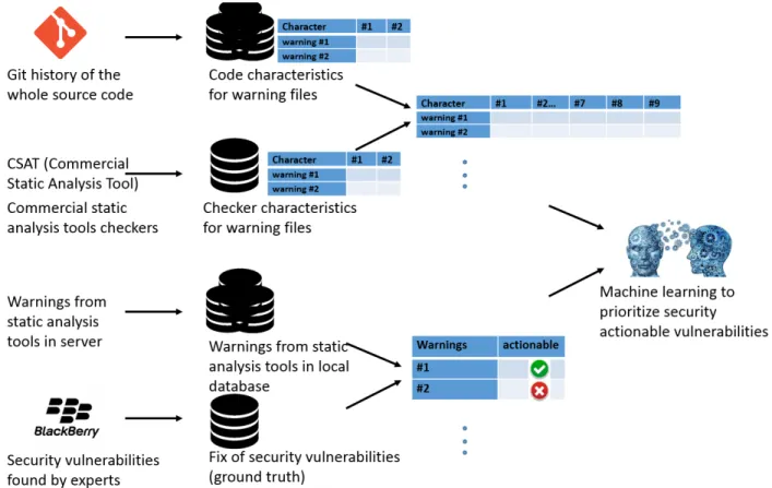
As shown in Figure 4.1, we do static analysis on several versions of the source code of three projects and then collect the generated warnings to create data sets for further training. Factors (features) of those warnings in the data sets were extracted from the source code repository and history. Ground truth refers to the facts of which class any given warning belongs to (e.g., actionable versus non-actionable). Ground truth labeling is performed manually by experts. Labelling is based on the existence of a warning over time in CSAT and code changes in the source code. Some of the warnings might be marked as

Fixed in CSAT without being fixed. With a large amount of features, feature selection is

important for classifier performance. Ensemble classifiers are built on selected features. Our approach uses feature extraction, feature selection, ground truth labeling, and statistical models to predict whether a warning is an actionable warning or not.

4.1 Commercial Static Analysis Tool Analysis

In our work, we use the CSAT tool to perform analyses on two open source projects (Apache HTTPD and MySQL) and one commercial project (BlackBerry internal project) with the regular setting of checkers. We analyzed multiple versions of three different projects — Apache HTTPD, MySQL, and an internal proprietary project from Blackberry

(35)

Figure 4.1: Process of feature extraction, feature selection, ground truth labeling, and machine learning in Prioritizer

Source code: commercial projects and open-source projects Ground truth: label false positives or actionable warnings

(36)

— in turn. Five versions of the code from Apache HTTPD and nine versions of the code from MySQL are picked spreading over two years. Three versions of the source code from the proprietary BlackBerry project are picked spreading over half a year. Each of the projects has over 500,000 lines of code. The regular setting satisfies the need for detecting critical vulnerabilities without too many false positives based on experts’ experience from BlackBerry. It should be noted that, both MySQL and Apache HTTPD include third party libraries which are not maintained by the project development team. The source code of these third party libraries is included in our analyses for completeness as those third party libraries upgrade with the source code. For the proprietary BlackBerry project, due to the size of the project, only one of the major modules is analyzed by CSAT while all the other modules within the same project are ignored.

4.2 Data Sources and Feature Extraction

We chose our features based on experiences from experts in BlackBerry and other researchers. These features were extracted from four perspectives of the static analysis tools and the code where the warning was detected. First, we extracted some information from the static analysis tool as do the work of Ruthruff [38], Heckman [19], and Kim [22] for warning descriptions. Kim [22] found a strong correlation between warning severity and bugs. Second, work by Bell [36] utilized features from individual files and commit information. Heckman [19] added features from function level, package level, and project level of the warning for predicting actionability. Third, code complexity often leads to more security vulnerabilities in the code [31], [39]. Complicated code has a higher possibility of being attacked. Shin [40] noticed that code complexity is the most important factor among code complexity, code churn (history of code changes), and developer activity in their benchmarks. Fourth, Ruthruff [38] and Heckman [19] both proved relevance of code churn factors with the bug occurrences. Shin [40] proved relevant of code churn factors with security vulnerabilities.

The goal of feature extraction is to remove noisy features and extract more structural features such as code metrics from code repositories and factors from static analysis tools that have good discriminatory value. Code metrics are made up of file characteristics, source code factors, and churn factors. File characteristics include the files age which reflects how long ago the file was created. Source code factors include lines of code which count the total number of lines of code excluding blank lines and comments in a source code file. Churn factors include total changes of code prior to the warning was reported. By replicating previous research and extending it to experiment with more precise machine

(37)

learning and feature selection algorithms, these features were selected, as shown in Table 4.1.

Commercial Static Analysis Tool issues (warning) descriptorCSAT descriptor has 274 checkers for C/ C++ and 190 checkers for Java.

Code The code (issue code) refers to the unique abbreviated name assigned to a detected warning type. For instance, ABV.ANY SIZE ARRAY is the issue code and buffer overflow-unspecified-sized array index out of

bounds is the description.

Subcode Subcode refers to the unique abbreviated category name of a code. For instance, ABV is the subcode of code ABV.ANY SIZE ARRAY and stands for buffer overflow for array.

Severity Each checker has a severity from 1 to 4 with 1 being critical warning and 4 being review warning. The severity shows up with each warning is never changed with warnings status as each checker is bonded with a severity.

File characteristicsFile characteristics contain the properties of the files where warnings were reported.

File age The total days of time period between created date of the file and the date the warning was detected.

File programming language

Programming language the file was written in. The programming lan-guage is expressed as a number: +1(C/C++)/ -1(Java)

Sha date delta weeks

The total number of the weeks the file was released prior to the warning detection

Directory The top one, top two, and top three hierarchies of the directories of file path before file name. The top one hierarchy of the directories dis-tinguish source code of open source projects from third party libraries source code. If there are only two directories before the file, then the top three hierarchies would be the same as the top two hierarchies of the directories.

(38)

Source code factorsMetrics of source code and code characteristics together form source code factors. File length, lines of code (loc), and code indentation [21] show the complexity of code.

Depth The ratio of the distance from the top of the file to the line of the warning detection compared to the total lines of the file.

File length Total number of lines in the file including lines of code, empty lines, and comments.

Mean tab Mean tabs indented in the beginning of code. If there is not tab in the beginning of code, then mean tab would be zero.

Mean space Mean spaces and tabs indented in the beginning of code. If there is not space in the beginning of code, then mean space would be zero.

Churn factors Churn factors consider the history of code changes prior to the warnings detection calculated from development history.

Add loc Added lines of code in two weeks, three months, six months, nine months, and twelve months prior to the warning detection.

Del loc Deleted lines of code in two weeks, three months, six months, nine months, and twelve months prior to the warning detection.

Fre Frequency of the file been were touched in two weeks, three months, six months, nine months, and twelve months prior to the warning detection. Change total Number of total lines of code has been changed, which is the sum of added lines of code and deleted lines of code, in two weeks, three months, six months, nine months, and twelve months prior to the warning detec-tion.

Percentage (add loc perc, del loc perc)

Percentage of added/ deleted lines of code in the past three months compared to loc.

(39)

CSAT warnings descriptors

code Types of warnings CSAT detect

subcode Categories of the warnings CSAT detect

be-long to

severity Severity of warning types

File characteristics

file age, create date delta weeks The length of the time the file existed file programming language Programming language of the file sha date delta weeks The length of the time the file released

dir The top hierarchies of the file path

Source code factors

depth The ratio of distance of the warning to the

total length

indentation (mean tab, mean space) Spaces and tabs indented in the beginning of code

loc Lines of code

total lines Lines of the file

Churn factors: files

add loc Added lines of code prior to the warning

de-tection

del loc Deleted lines of code prior to the warning

detection

fre Frequency of modifications prior to the

warn-ing detection

change total Modified lines prior to the warning detection percentage (add loc perc, del loc perc) Percentage of added/deleted lines of code

prior to the warning detection

(40)

4.3 Experimental Datasets Labeling

For supervised machine learning models, the datasets require features in machine learn-ing and class that each row (warnlearn-ing) of the datasets belongs to. To have a ground truth to work from, we manually checked the elements in each dataset, and labeled each element with either actionable or non-actionable based on whether the element has been fixed ac-cording to the reported warning in later versions of the code. The labeling was performed by two individuals: the author and another employee from BlackBerry. In the case of disagreement, another BlackBerry employee decided on the label. Otherwise, we keep the class of the warnings as labeled.

CSAT marked all the warnings that disappeared in later analysis as “Fixed”, on the assumption that they disappeared from the code because they had been fixed by the development team. However, not all the “Fixed” warnings are addressed by performers regarding the warning reported issue. For instance, if the file where the warning has been deleted, CSAT would still mark the warning as “Fixed”. But in our opinion, this warning is non-actionable. We verified all the “Fixed” warning manually and labelled them with actionability. If a warning is marked as fixed by CSAT, and fixed by performers towards the warning, then we label it as actionable, vice versa.

For each project, a series of CSAT analysis were conducted on 5 to 10 versions of historical code. Datasets generation is very time consuming as we label the actionability of warnings manually. Therefore, we randomly select around 200 warnings from each of the project and label them to form our datasets. For Apache HTTPD, the total amount of warnings is 208 and 199 are selected, the confidence interval is 0.57 when the confidence level is 95% [41]. If the accuracy is 90%, then with 95% confidence level, the accuracy is between 89.43% (90 - 0.57) and 90.57% (90 + 0.57). For MySQL, the total amount of warnings is 1506 and 193 are selected, the confidence interval is 4.43 when the confidence level is 95% [41]. If the accuracy is 90%, then with 95% confidence level, the accuracy is between 85.6% (90 - 4.4) and 94.4% (90 + 4.4). For proprietary BlackBerry project, the total amount of warnings is 3668 and 200 are selected, the confidence interval is 3.07 when the confidence level is 95% [41]. If the accuracy is 90%, then with 95% confidence level, the accuracy is between 86.93% (90 - 3.07) and 93.07% (90 + 3.07).

All the repetitive warnings are removed from the datasets. If a warning is ever marked as fixed by CSAT in any later analysis, we explore the warning by hand and label it as actionable or inactionable. If a warning is never marked as fixed by CSAT in any of the later analysis, we mark the warning as inactionable (not acted on). It is possible that warning is fixed out of our scope of analysis. But it would be a subjective and biased decision to make about actionability by us.

(41)

If a warning is addressed due to the reason CSAT reported then it is actionable. Two ex-amples of actionable warning and non-actionable warning from CSAT analysis of MySQL.

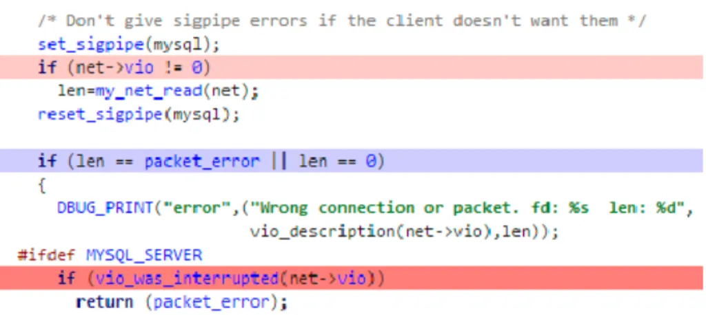
Figure 4.2: An example of a warning that labeled as actionable from CSAT analysis of MySQL

In Figure4.2, “net -> vio” is checked for “NULL”. However, later “net -> vio” is dereferenced without “NULL” checking. Logically, it is possible that “net -> vio” is “NULL” and get dereferenced again. In Figure 4.3, the validity of “net -> vio” is checked before usage. We label it as actionable because the warning is fixed for the potential vulnerability reason as CSAT reported.

Figure 4.3: The fix of the actionable labeled warning from CSAT analysis of MySQL In Figure 4.4, CSAT reported that “el -> el_line.buffer” is used after have been freed. The function “el_realloc” calls realloc function inherited from C. It doesn not automatically free the variable after calling. Thus the usage of “el -> el_line.buffer”

(42)

afterwards does not cause the problem CSAT reported. The warning which reported 4.4 is labelled as non-actionable.

Figure 4.4: An example of a warning that labeled as non-actionable from CSAT analysis of MySQL

4.4 Machine Learning Approaches

Langley [26] showed that there is no machine learning approach that works in all the fields. Therefore, we experiment with three different approaches so as to get the superior results. We apply machine learning models to the same datasets with three different approaches: machine learning classifiers, feature selection, and machine learning classifiers, as well as machine learning techniques for imbalanced datasets. The datasets consist of all the features from Table4.1and labeling of actionable or non-actionable. All the approaches are implemented in Java Weka API [18].

For each of the three approaches, seven machine learning classifiers are trained and evaluated in our study: Random Forest [3], Bayesian Network [2], KStar [8], SVM [4], Conjunctive Rules [18], Decision Table [24], and Logistic Regression [27]. Then the trained classifiers are evaluated with 5-fold cross-validation.

Random Forest [3], BayesNet [2], KStar [8], SVM [4], Conjunctive Rules [18], Decision Table [24], and Logistic Regression [27] are all popular machine learning models for various of tasks.

Random Forest [3] is an ensemble model that combines classification trees with a ran-dom bagging step. Originally, the classification trees are constructed by generating nodes that can best split the datasets. In a random forest, instead of using the best split nodes,

(43)

the random “feature bagging” step generates each node by the best among a subset of nodes. After the construction, the datasets that to be predicted go down each of the trees. Each of the trees gives an result and “vote” for the class.

Bayesian Network [2] is a directed acyclic graphical model that construct the dependen-cies of a dataset. It can be used for classification especially when features have conditional dependencies.

KStar [8] is a distance measure classification model that uses entropy to get benefits such as missing value. It is an instance-based learner that classify new coming data from classes of previous classified data that are similar to it. The distance measure is the transformation of transforming one instance to another.

SVM [4] mode treats datasets as points in space and generates a trained classification to ensure the gap between classes as far as possible. Four kernel models in SVM are included in our experiments: Linear, Polynomial, RBF (Radial basis function), and Sigmoid. If the trained classification kernel is specified as linear, then the generated trained classification is a linear model that separate different categories.

Conjunctive Rules [18] classifies the class from “AND” rule of features.

Kohavi [24] found that Decision Table works surprisingly well in some cases when datases include continuous features. Decision Table classifier [24] classifies datasets with a simple decision table. It selects a subset of features to generate a schema in the decision table. Then match the new coming data to the exact schema for the class. If no match is found, the majority class is returned.

Logistic Regression [27] measures the relationship of features and class wth a logistic regression. The model is modified in Weka to handle weighted datasets.

4.4.1 Machine Learning Classifiers

In the approach of machine learning classifiers, we train the seven classifiers with datasets that consist all of the extracted features from Table 4.1. Within the datasets, each row of the datasets is labeled with actionable or non-actionable as described in sec-tion 4.3. The classifiers are trained for a binary classificasec-tion and later evaluated with 5-fold cross-validation on the same training datasets.

(44)

4.4.2 Feature Selection and Machine Learning Classifiers

In the design of feature selection and machine learning classifiers, we select highly correlated subsets of features first and then apply machine learning classifications to the reduced datasets. There are seven strategies for correlated subset feature selection: Cfs-SubsetEval [17] and GreedyStepwise, CfsSubsetEval and BestFirst, InfoGainAttributeEval and Ranker, ClassifierSubsetEval and GreedyStepwise, ClassifierSubsetEval and BestFirst, ChiSquaredAttributeEval and Ranker, PrincipalComponent (Principal Component Anal-ysis) and Ranker.

CfsSubsetEval selects features that are correlated with the class with no intercorrelation among them. It excludes redundant features during screening and include the highly correlated features as long as they are not correlated with previous selected features.

InfoGainAttributeEval, Information Gain Evaluation in Weka, measures the features with their contribution to reduce the overall entropy. A good feature reduces the most entropy with the most information gaining. Information, also known as purity, represents the necessary information to classify a row in the datasets.

ClassifierSubsetEval evaluates subset of features on training data and estimates the “merit” of the subset with a classifier.

PrincipalComponent converts a set of features into a set of variables called principal components. In Weka, Principal Component Analysis is in usge with Ranker search. This can reduce the noise and redundancy of features.

GreedyStepwise performs a greedy forward or backward search in the feature set. It starts with no or all features and stops when no more features increase the evaluation. It implements steepest ascent search in Weka. In our experiments, we use greedy forward search.

BestFirst, Best-first search in Weka, searches the subsets of features forward from an empty set or backward from the full set of features. The search algorithm beam search is used in BestFirst in Weka. We use forward in our experiments.

Ranker ranks features by their evaluators such as Entropy.

One of the seven strategies first select a subset of correlated features. Then the new dateset that consist of subset of correlated features and actionablitily labeling is used to train one of the seven classifiers. The classifier is then evaluated with original dataset. In total, there are 49 combinations of seven feature selection strategies multiplied by seven classifiers. The trained classifier is later evaluated with 5-fold cross-validation.

(45)

4.4.3 Machine Learning Techniques for Imbalanced Datasets

Within the field of machine learning, there are two major approaches to dealing with imbalanced datasets: tweak the classifiers with cost-sensitive techniques and reconstruct the datasets with resampling techniques. Cost-sensitive techniques, cost-sensitive predic-tion, and meta-cost are three distinct techniques in cost-sensitive learning. Resampling techniques include resample datasets with over-sampling and under-sampling to balance the ratio of the datasets. Resampling techniques consist of over-sampling with replace-ment, over-sampling without replacereplace-ment, under-sampling (such as spread subsample), and Synthetic Minority Oversampling Technique (SMOTE) [5] [11].

In cost-sensitive learning, weights are assigned to different classes in the training datasets. These weights are applied in the machine learning process. Different from cost-sensitive learning, cost-sensitive predicting predicts the class with weights to increase the cost of misclassification. In meta-cost, the training data is reclassified from a bagging approach. The meta-cost uses bagging iteration for reclassifying training datasets and generates one classifier from the training datasets.

In the training of the seven classifiers, the cost matrix used by cost-sensitive learning, cost-sensitive predicting, and meta-cost are the same: one extra cost for false positives and ten extra cost for false negatives. The seven classifiers classify datasets on minimum cost after applying the cost matrix. These trained classifiers are evaluated by 5-fold cross-validation with the same datasets that they are used in training.

Over-sampling technique generates a random subsample of a dataset with or without replacement of instances from the minority class from the original dataset. Under-sampling such as spread subsample reduces the dataset by removing the instances from the majority class (binary classification). In addition, SMOTE shows a combination of over-sampling and under-sampling to achieve a better performance.

The reconstructed datasets from resampling are the same size with the original datasets with 5:1 ratio of majority class compared to minority class. Then the trained classifiers are evaluated with the datasets that are used in training with 5-fold cross-validation.

There is no guarantee that one of the approaches for imbalanced datasets work best for all the projects. Therefore, all the approaches are adopted to experiment and compare for our projects.

Case Studies of a Machine Learning Process for Improving the Accuracy of Static Analysis Tools