Improving Pure-Tone Audiometry Using Probabilistic Machine Learning Classification

(1)

Washington University in St. Louis

Washington University Open Scholarship

Engineering and Applied Science Theses &

Dissertations McKelvey School of Engineering

Summer 8-15-2017

Improving Pure-Tone Audiometry Using

Probabilistic Machine Learning Classification

Xinyu Song

Washington University in St. Louis

Follow this and additional works at:https://openscholarship.wustl.edu/eng_etds

Part of theBiomedical Engineering and Bioengineering Commons,Computer Sciences Commons, and thePsychology Commons

This Dissertation is brought to you for free and open access by the McKelvey School of Engineering at Washington University Open Scholarship. It has been accepted for inclusion in Engineering and Applied Science Theses & Dissertations by an authorized administrator of Washington University Open Scholarship. For more information, please [email protected].

Recommended Citation

Song, Xinyu, "Improving Pure-Tone Audiometry Using Probabilistic Machine Learning Classification" (2017).Engineering and Applied Science Theses & Dissertations. 310.

(2)

WASHINGTON UNIVERSITY IN ST. LOUIS School of Engineering and Applied Sciences

Department of Biomedical Engineering

Dissertation Examination Committee: Dennis L. Barbour, Chair

Steven E. Petersen Baranidharan Raman Mitchell S. Sommers Kurt A. Thoroughman

Improving Pure-Tone Audiometry Using Probabilistic Machine Learning Classification

by Xinyu Song

A dissertation presented to The Graduate School of Washington University in

partial fulfillment of the requirements for the degree

of Doctor of Philosophy

August 2017 St. Louis, Missouri

(3)

(4)

ii

List of Figures

Figure 1.1: A standard clinical audiometer. ... 4

Figure 1.2: Example of a clinical air conduction threshold audiogram. ... 5

Figure 1.3: Example of the clinical modified Hughson-Westlake procedure. ... 6

Figure 1.4: Example of a psychometric function. ... 14

Figure 2.1: Example of Bayesian inference. ... 26

Figure 2.2: Illustration of a latent function passed through a sigmoidal likelihood. ... 31

Figure 2.3: Illustration of the effects of a length scale hyperparameter. ... 34

Figure 2.4: A diagram of a standard active learning cycle. ... 38

Figure 3.1: Illustration of the machine learning (ML) audiogram technique. ... 48

Figure 3.2: Photo of the sound isolation booth used to conduct experiments. ... 49

Figure 3.3: Diagram of the automated ML audiogram procedure. ... 51

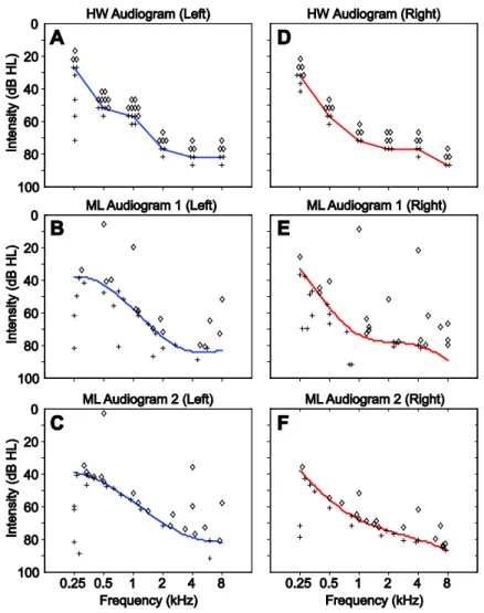
Figure 3.4: Sample plots of HW, ML1, and ML2 audiogram results. ... 55

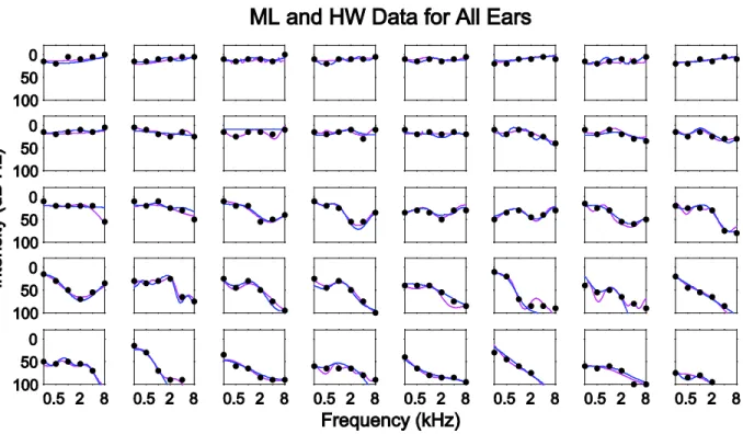
Figure 3.5: Agreement between ML and HW results for all valid ears. ... 56

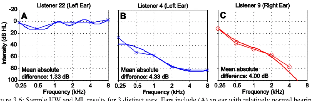
Figure 3.6: Sample HW and ML results for 3 distinct ears. ... 57

Figure 3.7: Direct comparisons of ML1, ML2, and HW threshold estimates. ... 60

Figure 3.8: Agreement between ML and HW as a function of algorithm iteration. ... 61

Figure 3.9: Normalized posterior variance as a function of algorithm iteration. ... 62

Figure 3.10: Data from Listener 17, who fell asleep during ML estimation. ... 65

Figure 4.1: Plot of 4 human audiometric phenotypes. ... 77

Figure 4.2: Examples of 1D PF estimation using PR and GPC. ... 82

Figure 4.3: Error in 1D α and β estimates for PR and GPC across all conditions. ... 83

Figure 4.4: Error in 1D PR and GPC α and β estimates for different β values. ... 84

(8)

vi

Figure 4.6: Direct comparison of 1D PR and GPC α and β estimates. ... 86

Figure 4.7: Sample posterior surface with samples and threshold/spread estimates. ... 88

Figure 4.8: Representative posterior distributions for four audiogram phenotypes. ... 89

Figure 5.1: Representative example of GPC inference using active sampling. ... 104

Figure 5.2: Representative posterior distributions for each sampling method. ... 105

Figure 5.3: Mean acquisition maps for each sampling technique. ... 106

Figure 5.4: Summary of active GP performance across all conditions. ... 107

Figure 5.5: Summary of active GP performance by audiogram phenotype. ... 108

Figure 5.6: Summary of active GP performance by β (spread) value. ... 109

Figure 6.1: Left- and right-ear GP human audiogram estimates. ... 119

Figure 6.2: Screenshot of the current website implementation for remote audiometric testing. 122 Figure A1.1: Error in 1D 50% point and IQR estimates for PR and GPC across all conditions. 141 Figure A1.2: Error in 1D PR and GPC 50% point and IQR estimates for different β values. ... 142

(9)

vii

List of Tables

Table 3.1: Summary of delivered samples for both HW and ML procedures. ... 54

Table 3.2: Differences between the ML audiogram estimate and the HW estimate. ... 58

Table 3.3: Test-retest reliability of ML audiogram. ... 59

Table 4.1: Absolute errors of 2D GP α and β estimates by number of samples. ... 90

Table 4.2: Absolute errors of 2D GP α and β estimates by value of β. ... 90

Table 4.3: Absolute errors of 2D GP α and β estimates by audiogram phenotype. ... 90

Table A1.1: Absolute errors of 2D GP 50% point and IQR estimates by number of samples. .. 143

Table A1.2: Absolute errors of 2D GP 50% point and IQR estimates by value of β. ... 143

(10)

viii

List of Abbreviations

1D: Unidimensional 2D: Two-dimensional

BALD: Bayesian active learning by disagreement dB: Decibels

dB HL: Decibels hearing level

dB SPL: Decibels sound pressure level GP: Gaussian process

GPC: Gaussian process classification GPR: Gaussian process regression

HW: Modified Hughson-Westlake procedure Hz: Hertz (cycles per second)

K-S: Kolmogorov-Smirnov test ML: Machine learning

MLAG: Machine learning audiogram PF: Psychometric function

(11)

ix

Acknowledgments

As I reflect back at the end of my long PhD adventure, I want to offer my gratitude to the many individuals without whom I could never have made it this far. First, I owe a huge debt of gratitude to my advisor, Dr. Barbour. I joined your lab in 2012 with many ideas but uncertain about the way forward. You helped me select and design projects that represented compelling technological and scientific advances, but took special care to ensure they were in line with my interests. Throughout my PhD trajectory, you’ve trusted me to forge my own path forward in research, but offered much-needed incentives and structure when appropriate. You have always been supportive not only of my scholarly endeavors, but also of my many interests outside of the laboratory; I’ve very much enjoyed sharing them with you. I am incredibly fortunate for the opportunity to work with and learn from a supportive, compassionate mentor like you.

The Barbour Lab has been filled with individuals who have had a profound impact on me not only as a scientist, but also as a person. To my labmates and fellow PhD candidates Jeff, Ruiye, and Wensheng: We all started at Washington University around the same time, and now, after completing our PhD journeys together, I feel like we are family. It goes without saying that you’ve been brilliant scientific peers, but I’ve also really appreciated our many non-work-related conversations on anything from politics and technology to entertainment and crazy start-up ideas (and at times, just listening to me complain). Your support and comradery have meant so much to me, and you have truly brightened my graduate school experience. To our post-docs, Noah and Ammar, and our lab technician, Kim: I’ve always looked up to you as role models of how to conduct scientific research, and I’m very thankful for all of the help and advice you’ve provided

(12)

x

during my time here. Of course, I would be remiss not to mention the energy and humor you’ve brought to the lab, always making this workplace a genuinely fun place to be.

I’ve been incredibly fortunate to have the support of some wonderful faculty members through my graduate school experience: Dr. Petersen, Dr. Raman, Dr. Sommers, and Dr. Thoroughman. From my qualifications exam (when I really had no idea what I was doing) to my Project Building presentations (when I was way too ambitious with my proposed research) to my thesis proposal (when I really thought I finally had my project figured out) and now, my defense, you have been there with me every step of the way. As my doctoral project has evolved over the years, your encouragement, insight and advice have always illuminated the way forward. I would not be where I am today without your gracious guidance and support.

This work could not have been completed without the help of two computer science professors. To Dr. Weinberger: I still vividly remember that particular machine learning class in spring 2014 when you first introduced Gaussian processes and active learning. I had originally thought that applying those techniques to audiometry would be a small side project, but it quickly took on a life of its own. To Dr. Garnett: I am truly fortunate for the opportunity to work with and learn from you. Your Bayesian methods courses have helped immensely in my basic grasp of the concepts, and whenever I still didn’t understand something (which was often!), you’ve always taken the time to patiently and thoroughly offer your insight.

Over my 6 years as a PhD student, Washington University has offered a positive, collaborative environment for my studies. In particular, the highly interdisciplinary Cognitive, Computational and Systems Neuroscience (CCSN) pathway has been instrumental in influencing how I think about science, and I am very thankful for my professors and fellow students in that pathway. I

(13)

xi

would also like to acknowledge my funding sources: the American Hearing Research Foundation (AHRF), the Center for Integration of Medicine and Innovative Technology (CIMIT), and Washington University in St. Louis. The research in this thesis would not have been possible without your generous support, for which I will always be grateful.

Within the BME department, I would like to thank Dr. Yin and Dr. George, the two department chairs during my time here: you have always been encouraging and have helped shape this department into the supportive, nurturing place it is has been. I owe so much gratitude to the department staff, Karen, Kate, Glen, and Amanda: I’ve lost track of how many times I’ve run into your office desperately needing help on anything from a room reservation to a last-minute grant submission; you’ve never hesitated to assist me, no matter how busy you were.

Over its approximate three years of existence, this machine learning audiogram project has involved many brilliant minds across various disciplines: Kiron, James, Braham, and Jacob in computer science; Brittany and Rebecca in audiology; Nikki, Katherine, and Joey in engineering, and Danish in ENT. Each of you has brought unique skills and expertise to the project (in addition to your lively personalities), and I’ve learned a great deal from working with you all. I truly would not have gotten where I am now without all of your help along the way; thank you.

I would like to thank my teammates on the audiogame projects: Tommy, Qihan, Sumeet, Jeff, Brittany, David, Danny, and Alice, as well as my collaborators in the Central Institute for the Deaf: Brent, Elizabeth, Cathy, Shannon, and Nancy. While ultimately that work didn't make it into my main thesis, we accomplished some very exciting things and I’ve learned a great deal through working together (including how to program in Android!). I have no doubt that the hard work we put into this project has set the groundwork for exciting research to come.

(14)

xii

A special thank you to my friends in the online music and local game development communities. There is no doubt that, apart from my PhD work, making music and making games have been the biggest parts of my life for these past six years. During times when my research felt tedious or frustrating, I could always turn to these endeavors as a productive outlet for my creative energy. You guys have been amazingly supportive of everything that I do, and I've found (and continue to find) so much inspiration from your kindness, talent, and determination.

These acknowledgments would not be complete without thanking my family: my mom, my dad, my grandparents on both sides of the family, my brothers Eddie and Michael, and many others. From a young age, you have instilled in me the creativity, curiosity, discipline, and will to succeed that have shaped me into the scientist and individual I am today. No matter what paths I have pursued in life, you have never stopped believing in me. Your unwavering faith in my ability and your unconditional love are the greatest sources of inspiration in my life, and this doctoral work is truly the fruit of your selfless devotion over my 27 years.

Xinyu David Song

Washington University in St. Louis

(15)

xiii

(16)

xiv

ABSTRACT OF THE DISSERTATION

Improving Pure-Tone Audiometry Using Probabilistic Machine Learning Classification by

Xinyu D. Song

Doctor of Philosophy in Biomedical Engineering Washington University in St. Louis, 2017

Professor Dennis L. Barbour, Chair

Hearing loss is a critical public health concern, affecting hundreds millions of people worldwide and dramatically impacting quality of life for affected individuals. While treatment techniques have evolved in recent years, methods for assessing hearing ability have remained relatively unchanged for decades. The standard clinical procedure is the modified Hughson-Westlake procedure, an adaptive pure-tone detection task that is typically performed manually by audiologists, costing millions of collective hours annually among healthcare professionals. In addition to the high burden of labor, the technique provides limited detail about an individual’s hearing ability, estimating only detection thresholds at a handful of pre-defined pure-tone frequencies (a threshold audiogram). An efficient technique that produces a detailed estimate of the audiometric function, including threshold and spread, could allow for better characterization of particular hearing pathologies and provide more diagnostic value. Parametric techniques exist to efficiently estimate multidimensional psychometric functions, but are ill-suited for estimation of audiometric functions because these functions cannot be easily parameterized.

The Gaussian process is a compelling machine learning technique for inference of nonparametric multidimensional functions using binary data. The work described in this thesis utilizes Gaussian process classification to build an automated framework for efficient, high-resolution estimation

(17)

xv

of the full audiometric function, which we call the machine learning audiogram (MLAG). This Bayesian technique iteratively computes a posterior distribution describing its current belief about detection probability given the current set of observed pure tones and detection responses. The posterior distribution can be used to provide a current point estimate of the psychometric function as well as to select an informative query point for the next stimulus to be provided to the listener. The Gaussian process covariance function encodes correlations between variables, reflecting prior beliefs on the system; MLAG uses a composite linear/squared exponential covariance function that enforces monotonicity with respect to intensity but only smoothness with respect to frequency for the audiometric function.

This framework was initially evaluated in human subjects for threshold audiogram estimation. 2 repetitions of MLAG and 1 repetition of manual clinical audiometry were conducted in each of 21 participants. Results indicated that MLAG both agreed with clinical estimates and exhibited test-retest reliability to within accepted clinical standards, but with significantly fewer tone deliveries required compared to clinical methods while also providing an effectively continuous threshold estimate along frequency. This framework’s ability to evaluate full psychometric functions was then evaluated using simulated experiments. As a feasibility check, performance for estimating unidimensional psychometric functions was assessed and directly compared to inference using standard maximum-likelihood probit regression; results indicated that the two methods exhibited near identical performance for estimating threshold and spread. MLAG was then used to estimate 2-dimensional audiometric functions constructed using existing audiogram phenotypes. Results showed that this framework could estimate both threshold and spread of the full audiometric function with high accuracy and reliability given a sufficient sample count; non-active sampling using the Halton set required between 50-100 queries to reach clinical reliability,

(18)

xvi

while active sampling strategies reduced the required number to around 20-30, with Bayesian active leaning by disagreement exhibiting the best performance of the tested methods. Overall, MLAG’s accuracy, reliability, and high degree of detail make it a promising method for estimation of threshold audiograms and audiometric functions, and the framework’s flexibility enables it to be easily extended to other psychophysical domains.

(19)

1

Chapter 1: Introduction

“In general and irrespective of the age at which it develops, disabling hearing impairment has devastating consequences for interpersonal communication, psychosocial well-being, quality of life and economic independence.”

−Quotation from (Olusanya et al., 2014)

“The deployment of accurate, automated [audiometric] methods to allow reallocation of time toward doctoral level activities is not only desirable, it is imperative.”

−Quotation from (Margolis and Morgan, 2008)

1.1. Hearing Loss

Hearing loss is a critical public health concern. Over 360 million individuals worldwide are estimated to have disabling hearing loss (Pascolini and Smith, 2009; World Health Organization, 2012), accounting for approximately 5% of the world’s population. For individuals 65 years and above, the proportion of affected individuals rises to 1 in 3. In the United States, approximately 37.5 million adults 18 and older, 15%, report some degree of hearing loss (Blackwell et al., 2014; NIDCD, 2014), making it the most prevalent neurological disorder in the country.

Typical cases of hearing disability can be classified into two main categories: conductive and sensorineural hearing loss (Sataloff and Sataloff, 2005). Conductive hearing loss describes hearing loss that results from an interference of sound transmission through the external/middle to the inner ear, while sensorineural hearing loss describes hearing loss that results from damage in the inner ear (particularly hair cells) and/or the auditory nerve. There are numerous factors that

(20)

2

lead to hearing loss, including diseases such as otosclerosis (De Souza and Glasscock, 2003) and Ménière's disease (Ménière and Atkinson, 1961), ototoxic drugs or chemicals (Schacht and Hawkins, 2006), noise exposure (Rabinowitz, 2000), trauma (Fitzgerald, 1996), and age-related degeneration (presbycusis) (Robinson and Sutton, 1979).

Hearing loss represents a large worldwide burden of disease (Mathers et al., 2000; Cruickshanks et al., 2003; Olusanya et al., 2014) and can have a dramatic impact on quality of life (Mulrow et al., 1990; Dalton et al., 2003). For adults, hearing impairment can have detrimental impacts on relationships, social function, cognitive ability, emotional well-being, physical ability, and career trajectory (Weinstein and Ventry, 1982; Thomas et al., 1983; Chen, 1994; Wallhagen et al., 1996; Mohr et al., 2000; Strawbridge et al., 2000; Helvik et al., 2006; Helvik et al., 2009). Hearing disability can be even more detrimental for children, including the estimated 7.5 million affected children 5 years or younger (World Health Organization, 2012). Hearing loss in children can interfere with speech and language development (Yoshinaga-Itano et al., 1998; Blamey et al., 2001; Briscoe et al., 2001; Yoshinaga-Itano, 2003), making detection even more critical.

Conductive hearing loss is often correctable via surgical or pharmaceutical intervention, while sensorineural hearing loss is currently not reversible (Sataloff and Sataloff, 2005). However, treatments can often dramatically improve hearing ability and significantly enhance quality of life for impacted individuals (Appollonio et al., 1996; Cohen et al., 2004; Vermeire et al., 2005; Chisolm et al., 2007). Perhaps the most common treatment for hearing loss is the use of a hearing aid, a device that amplifies and processes environmental sound that can be specifically tuned for individual hearing losses (Sataloff and Sataloff, 2005; Katz et al., 2009). More severe sensorineural hearing losses are sometimes treated using cochlear implants, devices that replace

(21)

3

cochlear hair cells with direct electrical stimulation of the auditory nerve (Clark et al., 1979; Bond et al., 2009). Cochlear implantation has been particularly effective for improving language development in deaf children (Svirsky et al., 2000; Sharma et al., 2002). Research has also demonstrated promising results for using auditory or speech training to improve listening ability in hearing-impaired individuals (Sweetow and Palmer, 2005; Burk and Humes, 2008; Fu and Galvin, 2008; Henshaw and Ferguson, 2013; Tye-Murray, 2014).

Despite these treatment options, however, hearing loss remains an underdiagnosed condition, partially owing to the lack of hearing screening procedures in standard clinics (Bogardus Jr et al., 2003; Yueh et al., 2003), which leads to lack of awareness in affected individuals. Other factors include the social stigma associated with and the financial burden of hearing treatment (Kochkin, 1993; 2007); this is reflected in the very low prevalence of hearing aid use among individuals who could benefit from them (Popelka et al., 1998; Chien and Lin, 2012).

1.2. Methods for Hearing Evaluation

1.2.1. Pure-Tone Audiometry

Perhaps the most common method for clinical hearing evaluation is pure-tone audiometry, which serially presents pure-tones of varying frequency and intensity to locate subjects’ auditory thresholds, or the lowest intensities at which an individual can detect a pure tone for a given frequency (Stach, 2010). A set of pure-tone thresholds given for a select number of frequencies collectively form an audiogram, which acts as a summary of an individual’s overall hearing ability. In this thesis, we will refer to an audiogram (in the traditional clinical sense) as a threshold audiogram because they are inherently comprised of only threshold information. Figure 1.1 shows a photograph of a typical audiometer used to estimate a threshold audiogram.

(22)

4

Figure 1.1: A standard clinical audiometer. This device allows for manual delivery of highly-calibrated pure tones at standard audiological frequencies and a variety of sound levels.

A threshold audiogram typically consists of auditory thresholds provided at a select number of pure-tone frequencies: 250 to 8000 Hz in octave intervals, with intermediate or edge frequencies sometimes included (American National Standards Institute, 2004a; American Speech-Language-Hearing Association, 2005); this frequency range is similar to the frequency range important for speech (French and Steinberg, 1947) Thresholds are most commonly reported in decibels hearing level (dB HL), which are sound level measures relative to what is considered to be normal hearing (Katz et al., 2009; Stach, 2010). Relative to physical sound pressure level (dB SPL), each frequency has a different correction term in order to convert between SPL and HL (American National Standards Institute, 2004b). This conversion allows for threshold audiograms of normal-hearing individuals to be represented by a horizontal line at 0 dB HL.

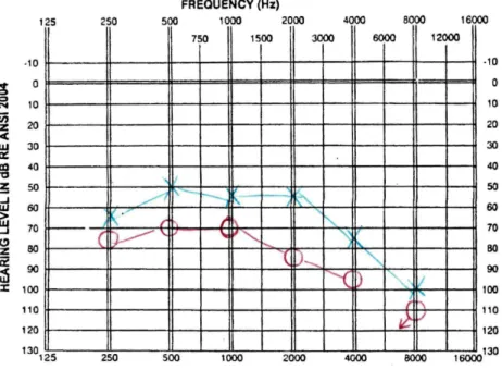
An example of a threshold audiogram can be seen in Figure 1.2, in this example providing thresholds for 6 audiogram frequencies. Thresholds for left and right ears, given by blue X and red O marks, respectively, are conducted separately for each individual. The pure-tone average,

(23)

5

or the mean of the measured thresholds at 500, 1000, and 2000 Hz, is often used as a quantitative summary of overall hearing ability. Categories for describing degree of hearing loss, including normal, mild, moderate, severe, and profound loss, are typically defined relative to the pure-tone average, although they may differ slightly depending on the reference (Goodman, 1965; Jerger and Jerger, 1980; Katz et al., 2009).

Figure 1.2: Example of a clinical air conduction threshold audiogram. Hearing thresholds in the right and left ears are denoted by red O and blue X marks, respectively. The red mark at 8 kHz was a no-response, wherein the subject

did not detect the stimulus provided even at the loudest intensity (110 dB HL in this case).

In accordance with established guidelines (American National Standards Institute, 2004a; American Speech-Language-Hearing Association, 2005), pure-tone audiometry is typically performed in clinic following the modified Hughson-Westlake procedure (Hughson and Westlake, 1944; Carhart and Jerger, 1959). The modified Hughson-Westlake (HW) procedure is an variant of the method of limits (Levitt, 1971; Kingdom and Prins, 2010; Gescheider, 2015) that adaptively selects pure tones to deliver in order to rapidly achieve an estimate for threshold.

(24)

6

Note that all references to the Hughson-Westlake procedure or HW throughout this thesis refer to this modified Hughson-Westlake procedure (Carhart and Jerger, 1959).

In the HW procedure, listeners are asked to indicate when they detect (even if minimally) the presence of a tone, typically by raising their hands or by pressing a button. Testing proceeds on a per-frequency basis beginning at 1 kHz. The intensity of the initial tone is chosen to be a sound level well above putative threshold (with additional steps taken if the initial tone is not detected). Thereafter, each time the listener detects a presented tone, its intensity is decreased by 10 dB for the subsequent presentation; each time the listener does not detect a tone, its intensity is raised by 5 dB for the subsequent presentation. This adaptive rule is followed for a certain number of reversals; threshold for the current frequency is considered to be the lowest intensity at which the subject perceives the tone approximately 50% of the time. This procedure is then repeated from the beginning additional frequencies and for the contralateral ear. Figure 1.3 shows an example HW run for detecting audiometric threshold at a single frequency.

Figure 1.3: Example of the clinical modified Hughson-Westlake procedure. This figure shows an example procedure at one frequency; this process is typically repeated at all 6-9 standard audiogram frequencies.

As a “2-up, 1-down” task, the threshold returned by this procedure corresponds to the 70.7% detection probability point on a listener’s psychometric function (Levitt, 1971). The HW method

(25)

7

is employed for both air conduction and bone conduction audiograms (Franks, 2001; Katz et al., 2009), which test distinct mechanisms of sound transmission and differ primarily in the type of transducer used. Masking of the contralateral ear is sometimes used for individuals who exhibit large inter-ear threshold audiogram differences, which helps to account for high-intensity tones being detected by the non-test ear (Katz et al., 2009; Stach, 2010).

Pure-tone threshold audiograms provide data that enables healthcare professionals to diagnose specific disorders (which often show loss localized to certain frequency ranges), screen for hearing disability, and monitor hearing changes over time, among many other applications (Katz et al., 2009; Stach, 2010). The adaptive Hughson-Westlake procedure has been a staple for hearing assessment for decades; its steps are easy to follow and it can be quite efficient in the hands of experienced audiologists. It has an accepted test-retest reliability of approximately 5 dB HL (Jerlvall and Arlinger, 1986; Fausti et al., 1990; Stuart et al., 1991; Schmuziger et al., 2004; Katz et al., 2009), which is reasonably high for most screening purposes.

However, HW pure-tone audiometry has several disadvantages. Perhaps the most striking is that these manually conducted pure-tone audiograms are highly time- and labor-intensive for medical professionals as a whole. It is estimated that annually, audiologists collectively spend around 2 million hours performing pure-tone audiometry alone (Margolis and Morgan, 2008), a rote task that does not leverage audiologists’ considerable expertise. Furthermore, the pure-tone audiogram provides only threshold data at any queried frequencies, with no information provided for intermediate frequencies. Although threshold audiograms such as Figure 1.2 linearly interpolate between measured thresholds for display purposes, no systematic estimate is provided for intermediate frequencies. The HW algorithm, while designed to quickly converge on

(26)

8

threshold, exhibits inefficiencies such as multiple high-probability stimuli being presented for each frequency (although this can be mitigated somewhat by a skilled audiologist) and identical stimuli presented repeatedly near threshold. Finally, the HW procedure is highly predictable, which facilitates the intentional subversion of test results by noncooperative listeners.

1.2.2. Alternatives to Manual Pure-Tone Audiometry

Automated Audiometry

In parallel to the development of adaptive conventional approaches like the one described above, automated audiometry methods have been developed for clinical audiometry, with the earliest form designed by Georg von Békésy in the late 1940s (von Békésy, 1947). Many computerized audiometric methods designed to ensure consistency and save labor have been developed, with some employing a method of adjustment similar to Békésy’s technique but most recent methods using a method of limits resembling the HW algorithm (Ho et al., 2009; Margolis et al., 2010; Swanepoel et al., 2010; Mahomed et al., 2013). Even with ready access to powerful digital computing technology today, however, automated audiometry sees relatively little use in clinical diagnostic settings, with most audiograms still obtained manually (Vogel et al., 2007).

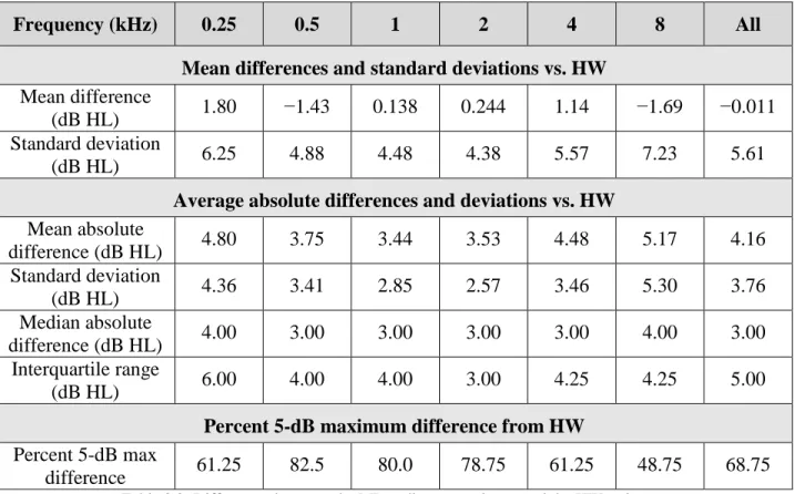
A recent exhaustive review and meta-analysis was conducted of techniques developed for automated threshold audiometry (Mahomed et al., 2013). A wide range of automated techniques produced audiograms generally comparable to manual audiograms, with an absolute average difference of 4.2 dB HL and a standard deviation of 5.0 dB HL (n = 360). Test-retest reliability among these automated methods demonstrated an absolute average difference of 2.9 dB HL and a standard deviation of 3.8 dB HL (n = 80). As a comparison, manual threshold audiometry in the reported studies produced an absolute average difference of 3.2 dB HL and a standard

(27)

9

deviation of 3.9 dB HL (n = 80). These studies indicate that computerized automation of pure-tone audiometry procedures yields threshold audiograms comparable in value and test-retest reliability to conventional manual procedures. However, the majority of automated techniques reviewed utilized adaptive techniques (including automated versions of the HW algorithm itself), which share many limitations with traditional pure-tone audiometry, particularly in performing inference one frequency at a time and reporting thresholds only at those points.

Sweep-Based Audiometry

Sweep-based audiometry is one alternative technique to adaptive methods that addresses the disadvantage of having data only at discrete frequencies. The first application of sweep-based audiometry was known as Békésy audiometry (von Békésy, 1947) and was application of the method of adjustment (Levitt, 1971; Gescheider, 2015). Listeners control the intensity of a pure-tone stimulus and are instructed to repeatedly increase its intensity until audible, then decrease its intensity until inaudible. The tone gradually sweeps across frequency in the meantime, allowing the final estimate to trace continuously across the threshold of hearing (von Békésy, 1947; Stach, 2010). A more recent implementation of sweep-based audiometry is Audioscan®, which uses a series of iso-intensity sweeps across frequency at varying intensities to trace out a high-resolution threshold curve (Meyer-Bisch, 1996; Ishak et al., 2011).

Because these sweep-based techniques trace out relatively continuous threshold curves along the frequency dimension, they have been shown to successfully identify various hearing pathologies that have been difficult to detect using discrete pure-tone audiometric approaches (Jerger, 1960; Zhao et al., 2002; Zhao et al., 2014). Despite this advantage, however, these techniques do not currently see substantial use in the clinic. One major reason is the lengthened testing time

(28)

10

required compared to conventional PTA, particularly with sweep rates that are sufficiently slow to be comfortable for listeners (Ishak et al., 2011). Furthermore, substantial engagement by the listener is required, which could lead to inefficient acquisition, inaccuracies, and/or intentional misrepresentation.

Bayesian Audiometric Techniques

Several more recent methods have taken a Bayesian approach to estimating pure-tone threshold audiograms, incorporating prior information from existing threshold audiogram shapes to inform optimal sequential selection of tones for efficient audiogram estimation (Özdamar et al., 1990; Stadler, 2009). The first approach uses a small database of weighted candidate audiometric patterns and iteratively selects the next tone at the frequency exhibiting maximum variance among patterns (Özdamar et al., 1990). Initial pattern probabilities are chosen according to prevalence of that pattern in the population, and probabilities are updated each iteration. A more recent method uses a Gaussian mixture model and a chosen utility function to select the optimal query point by maximizing the expected utility (Stadler, 2009). Similarly to the previous method, the model is initially trained using prior data (in this case, a database of 100000 threshold audiograms), and model parameters are updated after each observation.

Both Bayesian techniques have demonstrated efficiency and accuracy in estimating audiograms for simulated and human listeners (Özdamar et al., 1990; Eilers et al., 1993; Stadler, 2009; Guan, 2011). However, like traditional adaptive methods, these methods limit the frequencies queried to the standard 6-9 audiogram frequencies, with no systematic estimates provided for intermediate frequencies. An extension of these Bayesian techniques to form a more continuous

(29)

11

threshold estimate across frequency could provide the high resolution associated with sweep-based techniques while maintaining the stimulus selection efficiency of adaptive techniques.

Self-Diagnostic Tools

In more recent years, particularly with the rise of mobile smartphone technology, a number of non-clinical diagnostic tools for the end user have emerged. These tools have been deployed for many platforms, including landline phone (Watson et al., 2012; Williams-Sanchez et al., 2014), Internet browser (Bexelius et al., 2008; Molander et al., 2013), and the increasingly common mobile electronic device (Szudek et al., 2012; Handzel et al., 2013; Swanepoel et al., 2014; Saliba et al., 2016). These self-diagnostic tools are much more accessible than traditional forms of hearing diagnosis; individuals are able to utilize these tests on their own personal computers or smartphones without the need to visit a specialty clinic. However, studies on these techniques have primarily demonstrated their utility as a screening rather than detailed diagnostic tool, making their current implementations unlikely to replace standard clinical methods.

Physiological Measures

In addition to psychophysical tests, certain physiological measures are sometimes recorded in-clinic to gauge hearing ability. One widely used physiological measure is the auditory brainstem response (ABR), a subclass of auditory evoked potentials and a neurophysiological response that can be detected with scalp electrodes (Jewett et al., 1970; Hecox and Galambos, 1974). The ABR has been shown to reflect the pure-tone threshold audiogram in certain frequency ranges and is particularly useful in diagnosis of certain functional disorders, such as acoustic tumors (Hecox and Galambos, 1974; Selters and Brackmann, 1977; Stapells and Oates, 1997). A second common measure is otoacoustic emissions (OAEs), which are low-intensity, frequency-specific

(30)

12

sounds generated from the cochlea that occur both spontaneously and in response to delivered stimuli (Kemp, 1978; Probst et al., 1987; Probst et al., 1991). Because they reflect the integrity of hair cells, OAEs reflect overall hearing ability to some extent, and are useful in monitoring of potentially ototoxic treatment (Gorga et al., 1997; Dorn et al., 1999).

Both the ABR and otoacoustic emissions have proven particularly successful in assessing the hearing ability and sensitivity of young children who do not have the capability of performing pure-tone audiometry (Katz et al., 2009; Stach, 2010). However, these physiological measures have seen comparatively lower employ relative to pure-tone audiometry due to lower sensitivity, higher test complexity, and increased testing time.

1.3. Psychometric Functions

Psychophysics describes the relationship between physical and perceptual processes, quantifying a subject’s perception while a sensory stimulus feature is systematically altered (Fechner, 1860). This relationship is traditionally described using a psychometric function (PF), which describes a subject’s task performance as a function of a physical variable or variables. For instance, in pure-tone audiometry, the sensory domain consists of pure-pure-tone auditory stimuli, and stimulus features being manipulated are the frequency and intensity of these pure tones. The full PF across the variable space captures not only a subject’s thresholds, but also the degree of uncertainty of a subject’s performance around those thresholds. For instance, research has hypothesized higher levels of internal noise in children versus adults for pure-tone detection and discrimination tasks (Allen and Wightman, 1994; Bargones et al., 1995; Buss et al., 2006; 2008); this effect across frequency/intensity space could be captured using the full audiometric PF.

(31)

13

Psychophysical tasks can be assigned a threshold below which successful task performance is considered unreliable and above which performance is considered reliable, such as the 70.7% audiometric threshold returned by the HW procedure. However, psychophysical responses are not absolute; for instance, a listener may still detect a tone played slightly below the reported threshold. To describe this inherent uncertainty, we typically assign a detection probability to each stimulus describing an individual’s performance at that stimulus.

For certain stimulus parameters, the subject’s detection probability increases with increasing value. For example, as the intensity (sound level) of a pure-tone stimulus increases, a listener will detect it with higher probability. The relationship between a psychometric variable (for which performance increases with increasing value) and a subject’s response probability can be described using a unidimensional (1D) PF. For a PF on a psychometric variable, we typically model the response probability as a sigmoidally increasing function with stimulus value (Klein, 2001; Kingdom and Prins, 2010; Gescheider, 2015).

A 1D psychometric function is typically characterized using two main parameters: threshold α and spread β. The threshold α corresponds to the point of inflection and describes the stimulus level for which performance is halfway between the highest and lowest values. The spread β characterizes the degree of uncertainty around threshold; a higher value of β lengthens the transition region where response probabilities are not at the minimum or maximum values. (Note that the definition of β varies between sources; β is sometimes used to describe slope, the inverse of spread. In this thesis, we consistently use β to describe spread.)

An example of a psychometric function can be seen in Figure 1.4. For a detection task, in which subjects respond when they detect a stimulus but are not forced to make a choice at each

(32)

14

presentation (Fechner, 1860; Kingdom and Prins, 2010), the idealized minimum and maximum response probabilities take values of 0 and 1, respectively. Threshold α describes the point of maximum uncertainty, where detection probability is 0.5. Spread β quantifies the change in stimulus level required to produce a particular change in probability. For non-detection tasks such as n-alternative forced choice (Fechner, 1860; Kingdom and Prins, 2010) or to account for or lapse or guess rates in detection tasks (Klein, 2001; Wichmann and Hill, 2001a), additional parameters λ and γ are sometimes added. However, because pure-tone audiometry is inherently a detection task, we will focus our development of PFs on the idealized detection case.

Figure 1.4: Example of a psychometric function. Threshold α corresponds to the point of inflection (at which detection probability is 0.5) and spread β quantifies the amount of response uncertainty around the threshold. For

this example, the cumulative Gaussian function (Equation 1.2) was used to generate the curve.

Many sigmoidal functions have been used to model PFs, two of the most common being the logistic and cumulative Gaussian functions, shown in Equations 1.1 and 1.2, respectively (Klein, 2001; Falmagne, 2002; Kingdom and Prins, 2010; Gescheider, 2015):

( )

1 1 exp x x α e ψ =  −  + _− _   , (1.1)

(33)

15

( )

1 2 2 1 exp 2 x _z x α dz e e π −∞  _ ₋ _    ψ = _{− } _  _ _   

∫

, (1.2)

where x is stimulus level, ψ

( )

x = p y

(

=1x

)

is detection probability, and z is a variable of integration. Both equations constrain the detection probability ψ

( )

x to the probabilistic range

0,1

 

 , with ψ

( )

x monotonically increasing with increasing x. The α parameter determines the location of the 50% point and the β parameter adjusts the relative shallowness of the sigmoid. Standard parametric choices of 1D PF models are a subset of generalized linear models (McCullagh and Nelder, 1989), which are comprised of a linear predictor transformed with a monotonic link function.

Many if not most real-world psychophysical phenomena of interest, however, are inherently multidimensional, with more than one variable that effects change in subjects’ performance. In pure-tone audiometry, for instance, listener performance is affected by both the frequency and intensity of the delivered tones. In addition to psychometric input variables, multidimensional PFs often include one or more non-psychometric variables, against which detection probability does not systematically increase. For pure-tone audiometry, the non-psychometric dimension is frequency; unlike with intensity, increasing values for frequency do not systematically result in higher detection probabilities and in fact, describing the effect of frequency on a listener’s performance is a goal of audiometric testing. A limited number of multidimensional PFs have been characterized, including auditory filters (Patterson, 1976; Shen et al., 2014), external contrast noise functions (Lesmes et al., 2006) and visual fields (Heijl and Krakau, 1975; Bengtsson et al., 1997). The PFs in these cases are parameterized, though the mechanistic

(34)

16

justification for doing so could be limited. However, the pure-tone audiogram PF includes a non-psychometric frequency input variable for which any particular parametric justification is weak.

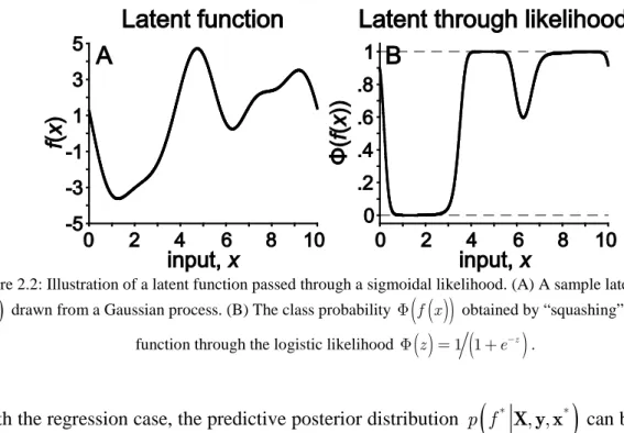
One elegant conceptualization of psychometric functions was proposed in (Kuss et al., 2005), in which any parametric 1D PF formulation can be decomposed into core and sigmoid functions. The core function contains the psychometric parameters α and β and is related to the detection probability; large positive core values produce detection probabilities close to 1; large negative core values produce detection probabilities close to 0, and core values close to 0 produce

detection probabilities near 0.5. The core function is often a linear function

(

x −α e

)

for psychometric variables to capture monotonicity, although it can take other parametric forms (e.g. logarithmic or polynomial) to account for non-psychometric variables. The sigmoid function is a

nonlinear transformation of the core function that “squashes” core values, which span

(

−∞ ∞,

)

, into the probabilistic range _0,1_. In this framework, the logistic function (1.1) can be

decomposed into core function

(

x −α e

)

and sigmoid 1 1

(

+e−x

)

. However, a limitation of this framework is that core functions must be specified parametrically, limiting its utility in cases for which parametric justification on a particular domain is weak or nonexistent.

1.4. Inference for Psychometric Functions

Psychometric functions have been a subject of study for decades. Research regarding PFs can be categorized into two broad topics: 1) methods to effectively estimate a PF from a set of data, and 2) methods to efficiently sample psychometric space to quickly arrive at an estimate. While there are now relatively standardized methods for fitting PFs, the question of how to most efficiently sample, particularly for multidimensional PFs, is still an active area of research.

(35)

17

1.4.1. Fitting Psychometric Functions

The problem of fitting psychometric functions to some set of observed data has overwhelmingly focused on the unidimensional case for psychometric variables (for which detection probability increases monotonically). Techniques for estimating 1D PFs typically assume a parametric form for the PF, typically a sigmoidal function such as (1.1) or (1.2).

Perhaps the most common method for fitting psychometric functions is maximum-likelihood regression (Morgan, 1992; Collet, 2003; Kingdom and Prins, 2010). In this method, binary repetitions at identical stimulus values are typically collapsed into a single proportion. Given the

observed binomial data  and a set of parameters θ, typically θ =

{ }

α e, for this application, we choose the set of parameters θˆ that maximizes the likelihood of observing these data given the parameters p

( )

θ . Often this maximum cannot be solved for analytically, so optimization methods such as the Nelder-Mead simplex method (Nelder and Mead, 1965; Kingdom and Prins, 2010) are employed to numerically locate the maximum.

Estimation of psychometric functions has also utilized Bayesian approaches (Bayes and Price, 1763; Jaynes, 2003), which accounts for prior beliefs on parameter distributions via a prior distribution (see Section 2.1.2). A Bayesian variant on the maximum-likelihood procedure, referred to as the constrained maximum-likelihood method (Treutwein and Strasburger, 1999), places prior distributions (in this particular work, beta distributions) on parameter values to obtain a point estimate of maximum-likelihood parameter values. Later work (Kuss et al., 2005) proposed a fully Bayesian treatment of 1D PF estimation, in which a full probability distribution

(36)

18

can be constructed over the parameters and point estimates can be obtained by minimizing some loss function, following standard Bayesian decision theory (Berger, 1985).

A limited number of parameter-free methods for PF estimation have been developed, which do not assume a particular parametric model as the form of the PF. One nonparametric technique uses the Spearman-Kärber method (Spearman, 1908; Kärber, 1931; Morgan, 1992), which can numerically estimate the moments of the PF (Klein, 2001; Miller and Ulrich, 2001). A second, more recent technique uses local linear fitting (Fan et al., 1995), which locally approximates a function using a Taylor expansion (Zychaluk and Foster, 2009). Although somewhat sensitive to method specifications, both techniques have demonstrated high accuracy and reliability for estimation of 1D PFs, even when compared to the appropriate parametric models (Klein, 2001; Miller and Ulrich, 2001; Zychaluk and Foster, 2009). However, nonparametric models for 1D PF estimation have seen very limited use in practice compared to parametric methods.

Frameworks for estimation of multidimensional PFs, which typically include at least one non-psychometric dimension, have been considerably scarcer. Certain parametric models have been developed for specific psychometric spaces, including the auditory filter (Patterson, 1974; 1976; Shen and Richards, 2013), the visual field (Heijl and Krakau, 1975; Bengtsson et al., 1997), the external noise contrast function (Lesmes et al., 2006), and elliptical-threshold PFs such as color difference detection (Kujala and Lukka, 2006). More flexible frameworks for multidimensional PF estimation have more recently been proposed, which specify particular parameterizations of threshold functions across non-psychometric dimensions (Vul et al., 2010; DiMattina, 2015; Watson, 2017). However, an incorrect choice of model parameterization can result in errors, and cases for which parametric justification is weak or nonexistent are not covered (Vul et al., 2010).

(37)

19

1.4.2. Sampling for Psychometric Functions

A related question to psychometric function inference is how best to select samples to efficiently produce accurate estimates of the PF. Traditionally, sampling for 1D PFs is accomplished using the method of constant stimuli, first proposed by Gustav Fechner (Fechner, 1860). In this method, a set of stimuli of varying stimulus levels are chosen such that they straddle a putative threshold value. Stimuli from this set are then delivered to the subject in a random order, with m repetitions delivered at n different stimulus values overall. When executed properly, the method of constant stimuli provides a well-spaced set of stimulus presentations that can capture psychometric behavior within a range of interest. However, downsides to this technique include sensitivity of PF estimation results to both the number of distinct stimulus levels delivered and to the number of repetitions at each level (often necessitating large numbers of samples to produce an accurate estimate), and the need for an additional procedure (e.g. a method of limits run) to determine the proper range for delivered stimulus values, and (Levitt, 1971).

To counteract the efficiency limitations of the method of constant stimuli, a number of adaptive procedural techniques have been developed for estimation of threshold only. A particularly well-established set of procedural methods is up-down methods, also called staircase methods (Dixon and Mood, 1948; Levitt, 1971; Kingdom and Prins, 2010). Up-down techniques follow the simple rule that if a stimulus is detected, the stimulus level for the next presentation should be decreased, and vice versa, until the test terminates. The standard up/down method uses the same step size for both stimulus increases and decreases, returning the 50% detection probability point (Dixon and Mood, 1948; Kingdom and Prins, 2010). Test termination typically occurs after a certain number of reversals, with the threshold estimate computed as the mean stimulus intensity across the last few trials containing a reversal (García-Pérez, 1998; Kingdom and Prins, 2010).

(38)

20

Modifications to the up-down method include transformed methods, in which some number of consecutive identical responses must be observed before adjusting stimulus level (for instance, 2 detections in a row before stimulus level is decreased) (Wetherill and Levitt, 1965; Levitt, 1971), and weighted methods, in which unequal step sizes are used for up vs. down (Kaernbach, 1991); these modifications correspond to different detection probabilities on the curve. A further refinement of up-down techniques was parameter estimation by sequential testing (PEST), which adaptively narrowed the step size of stimulus level changes to efficiently determine threshold (Taylor and Creelman, 1967; Findlay, 1978). Although these procedural techniques are designed to estimate thresholds only, a parametric fit can be performed to the set of stimuli and responses collected during the procedure using a fitting technique (Section 1.4.1); this strategy has been called a “hybrid adaptive procedure” (Hall, 1981; Leek et al., 1992).

A second class of adaptive techniques seeking 1D thresholds utilizes methods that have control over the exact stimulus placement for each delivery, rather than relying only on step size changes (Treutwein, 1995; Leek, 2001; Kingdom and Prins, 2010). The general framework involves at every iteration computing an estimate based on the data observed so far, then choosing the next sample point based on some value derived from the current estimate, typically to maximize some information measure. For example, the “best PEST” technique places each subsequent stimulus delivery at the current estimate’s 50% threshold value (Pentland, 1980). A Bayesian variant of this technique was proposed with QUEST, which uses the set of all trials collected so far as well as prior information to construct a posterior distribution and uses its mode, median or mean as the point estimate for threshold, which is sampled in the subsequent iteration (Watson and Pelli, 1983; King-Smith et al., 1994). Various updates on and variants of these “maximum-likelihood”

(39)

21

adaptive procedures have been developed for different stimulus spaces and test designs (Green, 1993; Dai, 1995; He et al., 1998; Leek et al., 2000; Leek, 2001; Linschoten et al., 2001).

The previously described adaptive techniques focus mainly on threshold, but a number of adaptive techniques for estimation of the entire PF (in particular, spread) have been developed. An early technique is adaptive probit estimation, which alternates between computing a probit fit given the current set of data (Finney, 1971) and selecting a new block of stimuli to deliver given the current estimate (Watt and Andrews, 1981). The modified ZEST technique, a Bayesian method, iteratively updates a 2-dimensional posterior probability distribution on threshold and spread parameters and selects the next stimulus level that minimizes the expected variance upon observing that trial (King-Smith and Rose, 1997).

Perhaps the most well-known technique for full 1D PF estimation is the Ψ-method (Kontsevich and Tyler, 1999). Like the modified ZEST technique, the Ψ-method iteratively updates posterior probabilities for threshold and spread. It then selects the stimulus intensity that maximizes the expected information gain after that sample is observed (i.e. minimizes the expected entropy). More recent techniques have refined this adaptive framework to better characterize optimal selection of points and to account for lapse and guess rates (Brand and Kollmeier, 2002; Shen and Richards, 2012; Shen et al., 2015). Extensions of these adaptive 1D PF estimation methods, particularly the Ψ-method, have also been applied to estimate multidimensional PFs (Kujala and Lukka, 2006; Lesmes et al., 2006; Lesmes et al., 2010; Vul et al., 2010; DiMattina, 2015).

1.5. Concluding Remarks

Clinical assessment of hearing ability is overwhelmingly conducted using manual HW pure-tone audiometry, costing millions of hours in labor each year for audiologists collectively. Automated

(40)

22

techniques have existed for decades but have primarily been variants on the HW procedure itself; other methods that have been developed, such as Bayesian techniques, are highly efficient but nonetheless produce estimates only at standard audiogram frequencies. Audiometric threshold estimates that are relatively continuous across frequency have been estimated using sweep-based methods, but such methods tend to be time-consuming and tedious for the listener.

Additionally, the full audiometric function (pure-tone multidimensional psychometric function) is almost never estimated in any capacity, which limits researchers’ ability to fully characterize certain forms of hearing disability for better diagnostic insight. Accurate and efficient techniques for estimating multidimensional PFs exist but all assume that the non-psychometric dimensions or threshold shapes can be parameterized in some form. However, the threshold curves for audiometric functions cannot be justifiably parameterized, as the particular shape of a threshold audiogram is itself indicative of the type of hearing disability.

In the work described by this thesis, we propose a method for estimating arbitrarily shaped audiometric functions using Bayesian machine learning classification, which we call the machine learning audiogram (MLAG). This technique does not require explicit parameterization of the audiometric function, instead encoding relationships between input points along any stimulus dimension, and can perform inference using binary response data typical of pure-tone detection tasks. This inherent flexibility allows for a variety of shapes to be encoded, including full audiometric functions and by implication, the associated threshold audiograms. While this thesis focuses on the particular application for pure-tone audiometry, the technique is general-purpose and can be extended to other psychophysical domains in a straightforward manner.

(41)

23

Chapter 2 introduces the concepts from probability theory and machine learning relevant to the work in this thesis. Chapter 3 describes MLAG applied to estimation of threshold audiograms in human listeners, comparing the results of our technique to traditional clinical methods. Chapter 4 characterizes the ability of MLAG to estimate multidimensional audiometric functions, including both threshold and spread, in simulated experiments. Finally, Chapter 5 extends the work of Chapter 4 to incorporate active sampling techniques, with the goal of improving efficiency.

(42)

24

Chapter 2: Machine Learning Background

2.1. Gaussian Processes

Parametric models, which have a deterministic form given a set of parameter values, are often employed to describe natural phenomena. However, many natural phenomena, such as weather patterns, heart rate over time, or neuronal firing activity, have a degree of randomness that are not well-described by deterministic models. Such phenomena are often better characterized using a stochastic process (Gubner, 2006), a collection of random variables that can describe the evolution of an inherently random process as a function of some independent variable.

The work in this thesis heavily employs the Gaussian process (GP), a mathematically convenient subclass of stochastic processes that encodes particular relationships between function values. While the GP has been conceptualized for decades, particularly in the geostatistics field where it has been referred to as “kriging” (Krige, 1951; Cressie, 1990), it has recently been adapted and further developed for machine learning applications (Rasmussen, 1996; Williams and Rasmussen, 1996; Gibbs, 1998; Williams and Barber, 1998; Rasmussen and Williams, 2006). This section provides a formal definition of the GP and describes how to use GPs for inference, as well as some details relating to GP construction.

2.1.1. Supervised Learning

Supervised learning describes a subset of machine learning techniques that aims to perform

inference on some system after observing a set of training data

{

(

)

}

1

, n i y_{i i}₌

= x

 , where x_i is a

(43)

25

corresponding to location x_i (Bishop, 2006; Hastie et al., 2009; Murphy, 2012). In supervised learning, we use the observed values  to train some model, encoding the system properties provided within the observations. We then use the trained model to make predictions on a vector

of unobserved features X*. For instance, the system we wish to perform inference on may be some unknown latent function f x

( )

, with y_i corresponding to a noisy function observation, i.e.

( )

i i

y = f x +ε. Supervised learning techniques stand in contrast to unsupervised learning techniques, which infer structure from “unlabeled” data that do not have corresponding categorical or numerical values.

A variety of techniques fall under the umbrella of supervised learning, including fully parametric estimators such as linear or logistic regression, statistical classifiers such as linear discriminant analysis, and nonparametric models such as k-nearest neighbor, support vector machines or neural networks. Gaussian process inference is a probabilistic method, which provides not only a

point estimate of a function values at each test point in X*, but a probability distribution describing its belief and uncertainty about the corresponding function value.

2.1.2. Bayesian Inference

A statistical framework that is particularly synergistic with the concept of supervised learning is the Bayesian technique. Broadly, the Bayesian framework encodes a set of beliefs about a system that can be updated in light of observed data. In function space, Bayesian inference begins by assigning a prior probability over functions that describes a belief about which functions are expected a priori, as well as some likelihood (observation model) that describes how observations are generated from the underlying function (Gibbs, 1998; Jaynes, 2003; Xiang and

(44)

26

Fackler, 2015). Given some observed data, Bayes’s Theorem can be applied to derive a posterior probability, which describes the updated beliefs about the function considering both the observed responses and the prior belief (Bayes and Price, 1763; Jaynes, 2003). Relative to supervised learning, the prior can be conceptualized as the initial state of the model, the observations upon which the posterior is conditioned as the training data, and the posterior distribution on some test

set X* as the post-training model prediction.

Figure 2.1: Example of Bayesian inference. (A) 5 sample functions drawn from a prior distribution on functions. (B) The posterior distribution after 4 observations are made, as well as 5 sample draws from this distribution. Solid lines

denote the mean, shaded gray areas denote 2 standard deviations about the mean, and dotted lines denote single draws from the corresponding distributions.

Figure 2.1 shows an example of inference using the Bayesian method. The prior distribution over functions, along with several draws from the distribution, is shown in Figure 2.1A. Figure 2.1B shows the posterior distribution after making several observations, coupled with a Gaussian error likelihood. Notably, the uncertainty of the posterior distribution is considerably decreased around the observations, limiting the space of possible functions to the subset that passes near the observed points. The 5 draws from the posterior distribution show functions from this subset.

(45)

27

2.1.3. Gaussian Process Regression (GPR)

Let f x

( )

be a latent function on an arbitrary input space x Î that we wish to model. A GP is a mathematically convenient mechanism to encode prior knowledge about f , which we can

update in light of observed data via Bayesian inference. Formally, a GP is defined as a collection of random variables (stochastic process), any finite subset of which jointly form a Gaussian

distribution. A GP is a natural extension of the multivariate Gaussian distribution 

( )

µ,Σ to infinite domains; like the multivariate Gaussian distribution, it is fully specified by its first two

moments: a mean function m

( )

x and a positive semidefinite covariance function K x x

( )

, ′ . The mean function accounts for the central tendency of the latent function while the covariance function accounts for the correlation structure of the latent function. Given m and K, the latent function f can be endowed with a GP prior distribution:

( )

(

( ) ( )

, ,

)

p f = µ x K x x′ . (2.1)

Consider a set of observations  =

{ }

X y, . Our GP prior on f implies a multivariate Gaussian distribution for the corresponding latent function values f = f

( )

X , but does not specify how these latent function values are related to our observations y. We must therefore use a likelihood function (observation model) to describe the relationship between the latent function and our

observations, or p

( )

y f . The likelihood function can be any arbitrary model, but in the standard regression case, the latent function f can be viewed as the underlying “true” behavior from

Improving Pure-Tone Audiometry Using Probabilistic Machine Learning Classification

Washington University Open Scholarship

Improving Pure-Tone Audiometry Using

Probabilistic Machine Learning Classification

Table of Contents

List of Figures

List of Tables

List of Abbreviations

Acknowledgments

Chapter 1: Introduction

1.1. Hearing Loss

1.2. Methods for Hearing Evaluation

1.2.1. Pure-Tone Audiometry

1.2.2. Alternatives to Manual Pure-Tone Audiometry

1.3. Psychometric Functions

( )

( )

∫

( )

(

)

( )

( )

(

)

(

)

(

)

(

)

1.4. Inference for Psychometric Functions

1.4.1. Fitting Psychometric Functions

{ }

( )

1.4.2. Sampling for Psychometric Functions

1.5. Concluding Remarks

Chapter 2: Machine Learning Background

2.1. Gaussian Processes

2.1.1. Supervised Learning

{

(

)

}

( )

( )

2.1.2. Bayesian Inference

2.1.3. Gaussian Process Regression (GPR)

( )

( )

( )

( )

( )

(

( ) ( )

)

{ }

( )

( )