Molecularly Imprinted Polymer Films
by
c
Andrew R. Way
A thesis submitted to the School of Graduate Stud-ies in partial fulfillment of the requirements for the degree of Master of Science.
Graduate Program in Scientific Computing
Memorial University
October 2019
Abstract
We present results of applying a feature extraction process to images of coatings of molecularly imprinted polymers (MIPs) coatings on glass substrates for defect detec-tion. Geometric features such as MIP side lengths, aspect ratio, internal angles, edge regularity, and edge strength are obtained by using Hough transforms, and Canny edge detection. A Self Organizing Map (SOM) is used for classification of texture of MIP surfaces. The SOM is trained on a data set comprised of images of manufactured MIPs. The raw images are first processed using Hough transforms and Canny edge detection to extract just the MIP-coated portion of the surface, allowing for surface area estimation and reduction of training set size. The training data set is comprised of 20-dimensional feature vectors, each of which is calculated from a single section of a gray scale image of a MIP. Haralick textures are among the quantifiers used as feature vector components. The training data is then processed using principal component analysis to reduce the number of dimensions of the data set. After training, the SOM is capable of classifying texture, including defects.
Lay summary
In a mass production environment, determining the quality of something usually in-volves finding defects. Take, for example, finding defects in bottles of beer. A defect could be a crack in the glass, an unusually wide neck, or an abnormally cloudy beer. Almost anyone walking the street could be asked to perform the task of finding such defects with minimal training. The problem is that people get tired, bored, or un-motivated pretty quickly. Sooner rather than later, the quality control worker begins to miss an increasing number of defective bottles. Human eyes, though attached to highly intelligent brains, tire quickly.
As an alternative, machines with the aid of computers can be used to find those same defects. Computers are really good at just one thing: adding numbers. Since they know how to add, they can also subtract, multiply, and divide. They’re also good at comparing numbers. Herein lies their strength; all operations performed by humans that are, at their root, basic arithmetic can be performed at inhuman rates by a computer. The video you stream on your computer, or the word processor you use at work are all provided to you by a computer performing basic arithmetic at unimaginable speeds. In addition to that, the memories of computers are virtually infallible; they do not forget what they know unless they are physically damaged or irradiated, or unless they are instructed by the user to forget it. They are the most reliable means of performing routine tasks day in and day out provided that we, the programmers, give them the right instructions. Providing this set of instructions such that the computer obtains sufficient independence and intelligence is the difficult task. In other words, machine eyes never tire but they can’t think for themselves.
This is the challenge we set out to solve for at least one scenario, one involving films of molecularly imprinted polymers (MIPs). To the average person, a MIP is just a “smear of paste” spread on a piece of glass. These smears of paste must be sold as a
MIP.
Acknowledgements
I would like to thank Memorial University of Newfoundland, ACOA, and NSERC for funding this research. I would like to sincerely thank Dr. Marek Bromberek for quickly supplying high quality imaging equipment, without which these results would not have been attainable. I would also like to thank Dr. Ali Modir for providing the MIPs. Furthermore, I would like to thank Dr. Mohamed Shehata of Memorial University of Newfoundland for providing initial source code for performing Hough transforms. Finally, I would like to thank my supervisors Dr. Carlos Bazan and Dr. Ivan Saika-Voivod for guiding this work.
Title page i
Abstract ii
Lay summary iv
Acknowledgements vi
Table of contents vii
List of tables xi
List of figures xii
1 Introduction 1
1.1 Overview . . . 1
1.2 Molecularly Imprinted Polymers . . . 1
1.3 MIP Production . . . 2
1.4 Quality Control Demands . . . 4
1.5 Computational Approach to Quality Control . . . 4
1.6 Overview of Thesis . . . 11
2 Methods 13
2.2 Canny Edge Detection . . . 15
2.2.1 Gaussian Filtering . . . 15
2.2.2 Intensity Gradients . . . 19
2.2.3 Non-Maximum Suppression . . . 21
2.2.4 Double Threshold . . . 22
2.2.5 Hysteresis-Based Edge Tracking . . . 22
2.3 Hough Transformations . . . 25
2.3.1 Homogeneous Coordinate Systems . . . 25
2.3.2 Applying a Hough Transform . . . 26
2.3.3 Sorting Lines . . . 26
2.4 Image Pre-Processing . . . 27
2.5 Detection of the MIP-containing Region . . . 29
2.6 Edge Trimming . . . 31
2.7 Calculation of MIP Side Lengths . . . 32
2.8 Rotation of the MIP . . . 33
2.9 Edge Quality . . . 35
2.10 Internal Angles . . . 37
2.11 Threshold-Based Defect Detection . . . 37
2.12 Calculation of Feature Vector . . . 39
2.12.1 Gray Levels . . . 40
2.13 Haralick Texture Features . . . 40
2.13.1 Gray Level Co-Occurrence Matrix . . . 40
2.14 Calculation of Intensity Resilience . . . 44
2.15 Principal Component Analysis . . . 47
2.16 Self Organizing Map . . . 52
2.16.2 Self Organizing Map Algorithm . . . 53
2.16.3 Training the SOM . . . 54
2.16.4 Neuron Labelling . . . 55
2.16.5 Classification of Image Sections . . . 55
3 Results 57 3.1 A Processed Set of MIP Films . . . 57
3.2 Detection of MIP Film Region . . . 59
3.3 Calculation of Geometric Properties . . . 62
3.4 Measurement of Edge Quality . . . 64
3.5 Feature Vector Creation . . . 66
3.5.1 Principal Component Analysis . . . 68
3.5.2 Feature Vector Values for Various Textures . . . 69
3.5.3 Initialization and Training of the SOM . . . 75
3.5.4 Labelling Neurons . . . 77
3.6 Texture Analysis . . . 79
3.7 Scrape Detection . . . 82
3.8 Statistics of a MIP Film Batch . . . 83
3.8.1 Statistics of Geometric Properties . . . 84
3.9 Statistics on Defect Detection . . . 88
3.10 Effect of Changing Haralick Feature Offset . . . 90
3.11 Effect of Increasing SOM Dimensions . . . 93
4 Discussion 95
5 Conclusions 98
Bibliography 100
A Matlab Code 104
A Image EXIF Meta Data 105
3.1 A table of the weights of each principal component and their corre-sponding features. . . 69 3.2 The z-scored principal component scores for each of the MIP film cells
shown in Fig. 3.19 . . . 70 3.3 The original feature vectors for MIP film cells A, B, C, and D shown
in Fig. 3.19 . . . 72 3.4 The original feature vectors for MIP film cells E, F, G, and H shown
in Fig. 3.19 . . . 73 3.5 The mean and standard deviation for each of the 20 features, calculated
using all 80,000 cells. . . 74 3.6 A comparison of defect detection accuracy between simple scrape
de-tection and the SOM-based approach. Each number in each column indicates the fraction of all MIP cells that were analysed, with the columns adding to one. True positive means a defect was correctly labelled, true negative means that a defect-free cell was correctly la-belled, false positive means the cell was labelled defective when it was not, and false negative means the cell was defective but was labelled as not defective. . . 83
List of figures
1.1 A flow chart illustrating the life cycle of a MIP film from production to usage. Reproduced with permission from Ref. [4]. . . 3 1.2 The computational pipeline used by the quality control system for MIP
films. . . 5 1.3 Raw image of the top of a cargo truck. Reproduced with permission
from Ref. [11]. . . 6 1.4 Canny edge image of the top of a cargo truck. Reproduced with
per-mission from Ref. [11]. . . 6 1.5 The accumulator space obtained from performing a Hough transform on
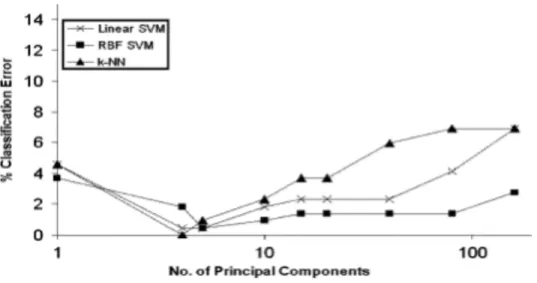
a Canny image of a truck. The four peaks correspond to the four sides of the trucks rectangle compartment. Reproduced with permission from Ref. [11]. . . 7 1.6 A plot of classification error, using a given machine learning algorithm,
versus number of principal components. Reproduced with permission from Ref. [18]. . . 9 1.7 An illustration of a trained SOM, where each square’s displayed image
indicates the type of wood image cell that is mapped to the square’s underlying neuron. Reproduced with permission from Ref. [21]. . . 10 2.1 Image acquisition equipment. . . 14 2.2 An example of a MIP film imaged using the described image capture
setup. . . 14
2.4 A side-by-side comparison of a corner of a MIP film before, on the left, and after, on the right, filtering is applied. . . 18 2.5 The gradient of a MIP film shown in Fig. 2.3b. . . 20 2.6 An image of a MIP in the non-maximum suppression step in the Canny
edge detection algorithm, where each white pixel indicates the corre-sponding pixel is a local maximum in the gradient image in Fig. 2.5a . 21 2.7 The log of the distribution of the magnitudes of the gradients from the
image shown in Fig. 2.5a, where the solid and dashed lines indicate the manually chosen upper and lower thresholds, respectively, used for the double threshold step. . . 22 2.8 The final Canny edge image of the MIP film shown in Fig. 2.3a. . . 24 2.9 Depiction of a straight line characterized by parameters ρ and θ in a
Cartesian coordinate system. . . 26 2.10 An image of a MIP film which has had its lower portion removed and
the image rotated. . . 28 2.11 An example defective MIP film which has had its four lines incorrectly
selected. . . 31 2.12 A MIP film, in the process of being trimmed, with its initially selected
lines shown in green and the partially trimmed line shown in red which will replace its parent line in the subsequent step of the line trimming algorithm. . . 32 2.13 A MIP film for which the geometry characteristics are overlaid on the
image . . . 33 2.14 An illustration depicting the lines and their corresponding θ values,
obtained from a Hough transform, for a MIP film. . . 34 2.15 The lines obtained from the Hough transform are shown in green, the
edge obtained from the Canny edge detector is shown in pink, and the search area to determine edge quality is shown in black. . . 36
2.17 A black and white image of Fig. 2.16 with threshold 0.75. . . 38
2.18 A simple 4×4 image with 4 possible gray levels. . . 41
2.19 An example of a MIP film with two regions of different texture which is highlighted. . . 44
2.20 An binary image of the MIP film shown in Fig. 2.19 . . . 45
2.21 Plots, and their corresponding image cells, which show how the total fraction of the image that is white decreases with respect to increasing threshold. . . 46
2.22 A two-dimensional data set plotted with respect to its two feature vari-ables. . . 48
2.23 A two-dimensional data set projected into a space spanned by its two principal component vectors. . . 49
2.24 An example of a train SOM consisting of several hundred neurons. Cells for each neuron that have defect class labels are highlighted by color depending on which class they belong to. . . 56
3.1 A picture of a good quality MIP film. . . 57
3.2 A picture of a defective MIP film. . . 58
3.3 A picture of an extremely defective MIP film. . . 58
3.4 A good quality MIP film with its outline overlay. . . 59
3.5 A defective MIP film with its outline overlay. . . 59
3.6 An extremely defective MIP film with its outline overlay. . . 60
3.7 A trimmed good quality MIP film. . . 60
3.8 A trimmed defective MIP film. . . 61
3.9 A trimmed, extremely defective MIP film. . . 61
3.10 A good quality MIP film with its geometry overlay. . . 62
3.11 A defective MIP film with its geometry overlay. . . 62
3.13 A close up of a MIP film corner. . . 64
3.14 A close up of a MIP film corner with an overlay indicating the quality of its edge. Cyan circles indicate that the underlying line segment is weak, and black rectangles indicate that the underlying line segment is too irregular. . . 65
3.15 A typical MIP film used to train the SOM. . . 66
3.16 A closeup of typical film texture from the MIP film in Fig. 3.15 . . . . 67
3.17 A closeup of a defect from the MIP film in Fig. 3.15 . . . 67
3.18 A scree plot of the principal component vectors obtained from applying PCA on the data set. . . 68
3.19 Various MIP film image cells taken from a set of 80,000 image cells. . . 71
3.20 An image of the trained SOM with example cells for each neuron. . . . 75
3.21 The neighbor weight distance plot for the trained SOM, with red indi-cating a large separation between neurons and yellow indiindi-cating mini-mal separation. . . 76
3.22 An image of the trained SOM with class labels for neurons associated with defects. . . 78
3.23 A good quality MIP film with flagged cells. . . 79
3.24 A defective MIP film with flagged cells. . . 80
3.25 An extremely defective MIP film with flagged cells. . . 81
3.26 A good quality MIP film with cells flagged based on the scrape detection algorithm. . . 82
3.27 A defective MIP film with cells flagged based on the scrape detection algorithm. . . 82
3.28 An extremely defective MIP film with cells flagged based on the scrape detection algorithm. . . 83
3.29 A histogram of surface areas of 145 MIP films. . . 84
3.31 A histogram of edge weakness of 145 MIP films, which is a measure, between 0 and 1, of what fraction of the total edge is considered too weak. . . 85 3.32 A histogram of edge irregularity of 145 MIP films, which is a measure,
between 0 and 1, of what fraction of the total edge is considered too rough. . . 86 3.33 A histogram of internal angles of 145 MIP films. . . 87 3.34 A histogram of defect rates, obtained from a SOM, in a batch of
ap-proximately 100 MIP films. . . 88 3.35 A histogram of defect rates, obtained from a scrape detection algorithm,
in a batch of approximately 100 MIP films. . . 89 3.36 An illustration of the offset used in calculating the Haralick texture
features for the original SOM. . . 90 3.37 An illustration of the offsets used in calculating the Haralick texture
features for a SOM. . . 91 3.38 A representation of a SOM that was trained using multiple offsets for
calculating Haralick texture features. . . 92 3.39 A representation of a trained SOM that contained more neurons than
the original SOM. . . 94
Introduction
1.1
Overview
Industrialization and urbanization have improved economies at the expense of clean natural water resources. In turn, they created the need for timely and efficient re-sponses for minimizing the negative effects of resulting accidents, or natural disasters that may affect fresh water supply. As a consequence, there is an increased interest in affordable, fast and easy-to-use methods for routine in situ analysis and moni-toring of markers of water contamination. Sensing systems that employ molecularly imprinted polymers (MIPs) are an attractive alternative for analysis of contaminants in aqueous media. In order to provide sufficiently high quality MIPs for commercial-ization, effective and efficient quality control processes must be put in place. In this thesis, we discuss such a system which consists of a computational pipeline of several methodologies based on image analysis.
1.2
Molecularly Imprinted Polymers
MIPs are synthetic materials that can be tailored to recognize specific compounds in complex samples by using molecular recognition similar to the “lock-and-key” mecha-nisms in biological receptors such as antibodies or enzymes [1][2][3]. Due to the MIPs molecular recognition abilities, MIPs are employed in applications involving the deter-mination of pollutants in water [4]. The most successful application of MIPs involve
solid phase extraction, a process known as molecular imprinted solid phase extraction (MISPE). Solid phase extraction is a process in which compounds that are suspended in a liquid mixture separate based on their physical and chemical properties. MIPs are used in tandem with this process. Xu [5] used MISPE with liquid chromatography to detect trace levels of a compound known as estrone in water, and achieved a limit of detection of 5.7 ng/L. Other applications of determination of pollutants include detection of water-soluble acid dyes [6], herbicides [7], and cyanide [8]. MIP films provide an effective and portable detection solution for these pollutants, which assists in mitigating their consequences on public health.
1.3
MIP Production
One of the most notable characteristics of MIPs is the simplicity of the fabrication process. This makes them an attractive component of water quality sensors that can be mass-manufactured by automated means. For their fabrication, MIPs are synthesized through polymerization of a functional monomer and a cross-linking agent around a template molecule (the compound of interest) [4] as shown in Fig. 1.1. Initial interactions take place in the pre-polymer mixture among the different components of the polymerization solution, in particular, the interaction between the template molecule and the functional monomer. When the template (or pseudo-template) is removed, we are left with a polymer showing complementary cavities in shape, size and functional groups to the target molecule. This is visible in the lower half of Fig. 1.1. The properties of the polymer can be tailored to suit specific compounds representing the water contaminant of concern.
Figure 1.1: A flow chart illustrating the life cycle of a MIP film from production to usage. Reproduced with permission from Ref. [4].
1.4
Quality Control Demands
MIPs have been developed in a range of formats to suit various applications, e.g., monoliths, beads, micro-spheres, and surface imprinted films [4]. Using MIPs in film format has many advantages for use in sensors for direct measurement of the compound bound to the film. There are current efforts to provide portable, selective and sensitive solutions for the characterization of water contaminants of concern by using MIPs in water monitoring products [9]. Therefore, there is a need for devising quality control methodologies for the manufacturing of new synthetic materials that form part of the sensing products. The proposed quality control methodologies involve the development of image processing and analysis techniques.
1.5
Computational Approach to Quality Control
The computational approach employed in this quality control system for MIP films is based on combining several methodologies into a single pipeline, shown in Fig. 1.2, which takes a color image containing a MIP film and outputs texture and geometry analyses.
Figure 1.2: The computational pipeline used by the quality control system for MIP films.
The first step of the pipeline involves the Canny edge detector [10] which finds edges within an image using a multi-step method later described. The result is a black and white image where the white pixels correspond to edges in the original image. The next step in the pipeline is to apply Hough transforms, which finds straight lines, to the image obtained from the Canny edge detector.
Figure 1.3: Raw image of the top of a cargo truck. Reproduced with permission from Ref. [11].
As an illustration, we consider the example provided by Xie and Zhou [11] in which Canny edges and Hough transforms were used to aid in the automated detection of a truck cargo compartment shown in Fig. 1.3. The Canny edge image is shown in Fig. 1.4.
Figure 1.4: Canny edge image of the top of a cargo truck. Reproduced with permission from Ref. [11].
After the Canny edge image was obtained, it was processed using the Hough trans-form algorithm. Hough transtrans-forms find straight lines by generating a set of lines, with varying orientation and distance from the origin, and counting the number of edge pixels each line intersects. Thus, the line that intersects and is co-linear with a long straight edge in the Canny edge image will have a high pixel intersection count, while other lines which intersect the edge but are not co-linear will have lower pixel in-tersection counts. The problem Xie and Zhou solved was finding which four lines corresponded to the rectangle of the cargo compartment shown in Fig. 1.4. The rect-angular compartment was found by finding a set of four lines which formed a rectangle.
These four lines appeared as peaks in the so-called “accumulator space” which dis-plays the edge pixel intersection count for each possible line, defined by parametersρ
andθ. The accumulator space is visible in Fig. 1.5. ρgives the perpendicular distance of the line from the origin of the image andθ defines the orientation angle of the line. For the compartment problem, this meant finding two pairs of lines that were parallel or, equivalently, having the same θ value. Additionally, the pairs themselves should be orthogonal to one another, which means having θ differing by 90◦.
Figure 1.5: The accumulator space obtained from performing a Hough transform on a Canny image of a truck. The four peaks correspond to the four sides of the trucks rectangle compartment. Reproduced with permission from Ref. [11].
This problem of finding a rectangle from a set of lines given some geometric con-straints is similar to the problem of detecting a MIP film within an image. MIP films have the constraint of being rectangular. Thus, by using a similar approach as Xie and Zhou, the rectangular outline of the MIP film may be found by finding which four lines create a four-sided polygon with a desired surface area, aspect ratio, and internal angles. Once the four lines are found, one may find the dimensions of the MIP film as well as remove parts of the image outside of the area enclosed to reduce the overall size of the image.
Once the geometry of the MIP film has been assessed, texture analysis is per-formed. Prior to performing texture analysis, each image needs to be translated into a feature vector, a collection of numbers calculated from features within the image. Zayed [12] used the well-known Haralick texture features in a statistical approach for
discriminating lung abnormalities. In their study, they found that certain Haralick texture features were significantly different in images containing tumors versus edema (or swelling). The images used for the data set were of cross-sectional computer-ized tomography scans of healthy lungs, lungs with tumors, and lungs with edema. Haralick features were chosen to be used for this thesis with the intent of finding abnormalities in MIP film texture, as they have stood the test of time as effective general purpose texture descriptors [13][14][15][16][17].
Once all desired features are calculated for sections of each image, the data set for texture analysis is finally formed. The next step in this computational approach is to reduce the dimensionality of the data set by performing principal component analysis (PCA). The aim of PCA is to find a set of uncorrelated feature vectors that point along the directions of the greatest variation in the original data set. The idea is that the original set of feature vectors describing the data set do not necessarily point in the direction of maximal variance because different features, generally speaking, are correlated. Howley [18] used PCA in a machine learning application and explored the effect it had on improving prediction accuracy and preventing the common problem of over-fitting due to too many dimensions. Howley found that in particular the support vector machine (SVM) classifier, which finds hyper planes that separate classes of data, and the k-nearest neighbors (k-NN) classifier, which assigns a class label to a data point based on the class labels of surrounding data points, achieved better results more efficiently when PCA was used. The error for these classifier methods decreased to a minimum for approximately 8 principal components, and subsequently increased with an increasing number of principal components used as shown in Fig. 1.6.
In general, the number of principal components chosen for the final data set is typically done using rules of thumb. According to Rea [19], several standard methods exist, one of which is the scree plot test which involves taking all components up to the point at which there is an “elbow” in the plot of the variance as a function of number of principal components used [20]. Once the principal components have been identified, they are examined by a subject specialist to determine if the principal components have meaning. In this research, the scree plot method is used.
Finally, texture analysis is performed by taking the reduced set of feature vectors and using them to train a sheet-like artificial neural network known as a self-organizing map (SOM). A SOM contains cells that become tuned to specific input signal patterns
Figure 1.6: A plot of classification error, using a given machine learning algorithm, versus number of principal components. Reproduced with permission from Ref. [18].
through an unsupervised learning process. Once trained, the cells within a SOM tend to become spatially segregated in such a way that cells that respond similarly to a specific input signal will reside within a domain. The spatial segregation of cells based on response to input signal is similar to how topology of the brain is related to function. Specific sections of the brain, when stimulated, disturb the function that is associated with that section. The disturbance may induce or inhibit some function, such as the movement of the hand. In other words, responses to input signals are spatially organized within the brain’s cerebral cortex. A SOM behaves similarly by having input signals induce a greater response with specific cells, or domains of cells, than others.
Figure 1.7: An illustration of a trained SOM, where each square’s displayed image indicates the type of wood image cell that is mapped to the square’s underlying neuron. Reproduced with permission from Ref. [21].
Niskanen [21] showed that a SOM could be trained on images of lumber to find and flag wood knots. The result of training the SOM is shown in Fig. 1.7. Each square cell corresponds to a neuron in the SOM, and the image of the wood shown is an example of an image cell that is mapped to that square. Evidently, wood knots tend to congregate near the bottom right corner of the SOM. Boundaries were created in the SOM for future classification, where if a new image cell was mapped within the lower-right boundary it could be classified as a wood knot. Thus, a SOM may be used for classification by assigning each domain a particular label. In the scenario of using MIP films, the usage will be similar; image cells of similar texture, such as scratches, should congregate in one section of the SOM. Subsequent to training, future image cells falling into that section of the SOM will be classified as scratches.
In addition to the literature reviewed above, a plethora of examples of applica-tions of machine learning using image data are reported in the literature. In par-ticular, machine learning finds extensive usage in quality control applications in the agricultural and fishing sectors, such as detecting the freezer burn rates in salmon via the TreeBagger classifier algorithm [22], detecting defects in raw potatoes using a convolutional neural network [23], measuring stress severity in soybeans using several different algorithms [24], and differentiating walnut shells from walnut pulp [25]. In the medical fields of research, back-propagation neural networks have been used for recognizing major sub-cellular structures in fluorescent microscope images of HeLa cells [26]. Additionally, quality identification of human induced pluripotent stem cell colony images have been achieved using support vector machines [27]. Finger print quality assessment has also been achieved using a SOM in-tandem with a random forest [28]. Finally, applications of machine learning on image sets exist in the mining and materials engineering fields as well. Applications include determining limestone ore grades using PCA and a neural network [29], recognizing patterns on images of metallurgical micro-structures using a random forest [30], and finally, the detection of residual traces of coating produced in metal welding via support vector machines [31].
1.6
Overview of Thesis
The remainder of this thesis is as follows. Chapter 2 is dedicated to describing the computational methodologies and features used to create the geometric and texture
analyses of the computational pipeline. It describes how the images are obtained, how the MIP film region is detected and measured using Canny edge detection and Hough transformations, how the quality of the MIP film is measured, how the texture features are calculated prior to using PCA, and how the SOM is used for texture analysis. Chapter 3 is dedicated to results on applying the computational pipeline to generate the geometric and texture analyses. Additionally, results on the effects of changing certain parameters, like the number of neurons in the SOM, are presented. Chapter 4 includes discussion on the performance of the quality control pipeline. Finally, Chapter 5 discusses and summarizes the results and outlines potential for future work.
Methods
2.1
Image Acquisition
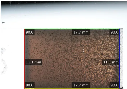
Images of the MIP films were taken with a Canon EOS5D II camera shown in Fig. 2.1a, a Canon 580 EX 2 Speedlight light source shown in Fig. 2.1b, and a Cactus v5 radio trigger for remotely triggering the image capture process. The camera used a Canon EF 100mm f/2.8 macro lens. The MIP films were placed on a large piece of glass. An example of a MIP film on this glass is shown in Fig. 2.2. Immediately below the MIP film is a ruler which was used to provide a scale for the quality control system. Behind the supporting piece of glass was the light source shown in Fig. 2.1b. Once the button on the remote was clicked, the light source illuminated the underside of the glass slide and then the picture was acquired. All metadata for the images, such as camera settings, are found in App. A.
(a) Canon EOS5D II [Source: Charles Lanteigne, https: //commons.wikimedia.org/wiki/ File:Canon_EOS_5D_Mark_II_ with_50mm_1.4_edit1.jpg]
(b) Canon 580 EX 2 Speedlight. [Source: KaiAdin, https://commons.wikimedia. org/wiki/File:Canon_Speedlite_580EX_ II_Front.jpg
Figure 2.1: Image acquisition equipment.
Figure 2.2: An example of a MIP film imaged using the described image capture setup.
2.2
Canny Edge Detection
Canny edge detection [10] provides structural information about an image while sup-pressing noise. The multi-step process is as follows:
1. Noise reduction using a Gaussian filter
2. Calculation of intensity gradients within the image 3. Non-maximum suppression
4. Double threshold
5. Hysteresis-based edge tracking Below, we explain each of these steps.
2.2.1
Gaussian Filtering
Since edge detection results are easily affected by noise, Gaussian filtering is applied to the images to perform noise reduction. Gaussian filtering works by first constructing a Gaussian kernel of size (2k+1)×(2k+1) given by
Gij = 1
2πσ2 exp−
(i−(k+ 1))2+ (j−(k+ 1))2
2σ2 ; 1≤i, j ≤(2k+ 1) (2.1)
and performing a type of averaging over pixel intensities with weights determined by the Gaussian kernel. For this thesis, σ = √2 and k = 6, and the Gaussian kernel is normalized such that its elements sum to one. Before filtering, the red-green-blue (RGB) image is first converted to a gray scale image by calculating a weighted sum of the RGB components using the formula
GLij = 0.299Rij + 0.587Grij + 0.114Bij (2.2) where GLij is the gray level, and Rij, Grij, and Bij are the components for each of the RGB channels for the pixel at row i and column j. This calculation eliminates the hue and saturation information of the original image while retaining the lumi-nance. Gaussian filtering is then performed by moving the kernel across the gray
scale version of the image and performing a convolution operation on each underlying (2k+1)×(2k+1) subsection of the image I, with the result being expressed as I0.
I0 =G∗I (2.3)
For example, a 5×5 Gaussian kernel is chosen to smooth the image shown in Fig. 2.3a. The kernel, which is just a matrix, is given by,
G= 1 159 2 4 5 4 2 4 9 12 9 4 5 12 15 12 5 4 9 12 9 4 2 4 5 4 2 (2.4)
The convolution operation is then performed on each 5×5 subsection of the image which results in the image shown in Fig. 2.3b. The most noticeable change between the two in this particular example is that the rough texture of the underlying glass slide dissipated.
(a) An un-processed MIP film.
(b)
The differences between the original image and the filtered image may be observed in Fig. 2.4, in which the same top right corner of the film from both Fig. 2.3a and Fig. 2.3b are expanded and compared side-by-side. The most noticeable difference is the removal of the edge pixels from the underlying glass slide, and the decreased spatial variation in pixel intensity in the filtered image.
Figure 2.4: A side-by-side comparison of a corner of a MIP film before, on the left, and after, on the right, filtering is applied.
2.2.2
Intensity Gradients
The intensity gradients, which is the rate at which the pixel intensity changes in a certain direction over some distance, is then calculated for the filtered image. The intensity gradients are calculated for the horizontal, and vertical directions, since an edge can point in either direction. The operator is a discrete differentiation opera-tor which approximates the gradient of the images intensity function. The operaopera-tor uses two kernels that are applied to the image’s subsections through a convolution operation as follows Mx= h −1 2 0 1 2 i ∗I0 (2.5) My = −1 2 0 1 2 ∗I 0 (2.6)
Above, Mx is the gray-scale image with intensity at each point calculated from the horizontal derivative ofI0, the original gray-scale image, at that same point. Similarly, My is an image constructed of pixel values which are the vertical derivatives of I0. The resulting gradient magnitude,M, and direction,Θ, are then calculated using
Θ= arctan (My,Mx) (2.7) and M= q M2 x+M2y (2.8)
which contain the gradient magnitude and direction for each point in the image. The result of applying this operation to the image, in which each pixel’s intensity is given byM, is shown in Fig. 2.5a.
(a) The image with pixels given by the gradient of the image in Fig. 2.3b.
(b) A color coded version of the gradient image of a MIP film shown in Fig. 2.5a. Black pixels have intensity between 0 and 0.05, red pixels have intensity between 0.05 and 0.2369, blue pixels have intensity between 0.2369 and 0.5922, and green pixels have intensity higher than 0.5922.
2.2.3
Non-Maximum Suppression
Using the gradient image obtained in Sec. 2.2.2, non-maximum suppression is applied. Non-maximum suppression is an edge thinning technique which seeks to remove points within an edge that are either noise or are superfluous. The goal of non-maximum suppression is to set every gradient to zero which is less than the local maximum where the most prominent edge points occur. The algorithm for non-maximum suppression is as follows:
1. Iterate over each pixel in the intensity gradient image
2. Compare the intensity of pixeli, j with the intensity in the positive and negative gradient directions
3. If the intensity is the local maximum, preserve it 4. Else suppress it
The positive gradient direction is given by Eqn. 2.7. The result of this step is depicted in Fig. 2.6, which shows a logical matrix (where each pixel is either 1 or 0). Each white pixel indicates that the pixel is a local maximum in the gradient image shown in Fig. 2.5a.
Figure 2.6: An image of a MIP in the non-maximum suppression step in the Canny edge detection algorithm, where each white pixel indicates the corresponding pixel is a local maximum in the gradient image in Fig. 2.5a
2.2.4
Double Threshold
Some edge pixels remain in Fig. 2.6 due to noise and color variation, even after apply-ing the first several steps of the Canny edge detection process. Thus, weak gradient pixels are filtered out using a double threshold step. In this step, two threshold values are determined either empirically or by using an algorithm. In this thesis, the up-per threshold was chosen based on inspection of the distribution of the magnitude of gradients which were obtained from images such as the one in Fig. 2.5a. The actual distribution is shown in Fig. 2.7. The upper threshold was set to where the distribu-tion began to decline at the end of the plateau. The lower threshold was manually set to be 0.4 times the upper threshold, which coincided roughly with where the dis-tribution tapered off and plateaued. These thresholds were used for all images within the data set.
Figure 2.7: The log of the distribution of the magnitudes of the gradients from the image shown in Fig. 2.5a, where the solid and dashed lines indicate the manually chosen upper and lower thresholds, respectively, used for the double threshold step.
2.2.5
Hysteresis-Based Edge Tracking
Weak pixels discovered in the step described in Sec. 2.2.4 require further work to determine whether they will be preserved or suppressed, while strong pixels are auto-matically included in the final Canny edge image. Weak pixels that are connected to
a blob, which is a collection of pixels that are connected through horizontal, diagonal, or vertical connections, that contain at least one strong pixel are preserved while the rest are suppressed. In Fig. 2.8a, a double threshold was used to classify each gradient pixel in Fig. 2.6. Blue pixels are weak, since they fall between the two thresholds, and any that are not connected to a strong, green pixel are removed from the image. Green pixels are strong, since they fall above both thresholds, and are preserved. The final result is shown in Fig. 2.8b.
(a) A color coded version of the local maximum gradient image of a MIP film shown in Fig. 2.6. Green pixels are strong, and blue pixels are weak according to the selected double threshold.
(b) A MIP film after being processed in the hysteresis-based edge tracking step in the Canny edge detection algorithm, where each white pixel indicates a final edge pixel.
2.3
Hough Transformations
Hough transformations [32] are applied to the Canny edge images obtained in the pre-vious step to find the presence of lines in a process facilitated by using a homogeneous coordinate system to represent lines. A valid line is one that passes through many Canny edge points. ρ is the perpendicular distance between the line and the origin and θ gives the direction of the line, as shown in Fig. 2.9.
2.3.1
Homogeneous Coordinate Systems
Lines in the xy plane can be represented using homogeneous coordinates denoted by l= (a, b, c) [32]. The equation of a line in this coordinate system is given by
x·l=ax+by+c= 0 (2.9)
Eq. 2.9 can be normalized so that l = (ˆnx,nˆy, ρ), where ˆn is the normal vector perpendicular to the line and ρ is its distance to the origin. This normal vector can be expressed in terms of the polar coordinate,θ, and is written as (cosθ,sinθ). Thus, using this homogeneous coordinate system a straight line can be represented in terms of coordinates θ and ρ. The straight line is expressed as
ρ=xcosθ+ysinθ (2.10)
from which the conventional equation of the line
y=mx+b (2.11)
may be derived, where m and b can be written in terms of ρ and θ as
m=−cosθ
sinθ (2.12)
and
b = ρ
sinθ. (2.13)
Figure 2.9: Depiction of a straight line characterized by parameters ρ and θ in a Cartesian coordinate system.
2.3.2
Applying a Hough Transform
A Hough transformation is a process by which voting occurs to determine the presence of plausible straight edges [32]. The result of a Hough transformation is the creation of the so-called accumulator space of the image, which is a three-dimensional space spanned by vectors represented byθ,ρ(as in Sec. 2.3.1), and the number of votes, C, for that line. The accumulator space is constructed by creating various combinations of θ and ρ, and counting the number of pixels intersected by the corresponding line, giving the number of votes. Straight edges are distinguished by having a high number of votes in the accumulator space. For example, a line that intersects a long row of points, i.e. an edge, will have a high number of votes and therefore will be represented in the accumulator space as a peak.
2.3.3
Sorting Lines
Straight edges in the image that are obtained from the Canny edge detection algo-rithm appear as peaks when processed with a Hough transform. Each of the peaks’ lines are characterized by parameters θ and ρ and Eqn. 2.10. To increase computa-tional efficiency, all chosen peaks are organized into two sets: one containing lines that are considered vertical, and another containing lines that are considered horizontal.
The logic that distinguishes horizontal lines from vertical lines is given by
Horizontal if 45◦ < θ≤135◦ or 225◦ ≤θ ≤315◦ Vertical if−45◦ ≤θ≤45◦ or 135◦ ≤θ≤225◦
The lines are sorted in order to reduce the number of combinations of lines used to find the four lines corresponding to the sides of the film. This also helps with finding which corner of the MIP corresponds to the intersection of two lines.
2.4
Image Pre-Processing
Prior to using the pipeline, the image is processed such that extraneous parts of the image are removed. This involves removing the lower part of the image which includes the ruler/support for the MIP. Since the ruler is in the exact same place in every picture, the equation of the line of the top of ruler may easily be found by manually picking the points at the left and right end of the ruler and determining its slope. From there, one may easily find the θ and ρ coordinates of the line. The θ
coordinate is used to rotate the image, and the ρ coordinate is used to determine up to what height of the image is kept in the resulting image shown in Fig. 2.10.
Figure 2.10: An image of a MIP film which has had its lower portion removed and the image rotated.
2.5
Detection of the MIP-containing Region
The MIP film is first detected to determine the geometry of the MIP film and then isolated to ensure only MIP film textures are used for subsequent machine-learning related steps. This is achieved by finding a set of four lines which forms the rectangle that coincides with the film. As discussed in Sec. 2.3.3, the set of all candidate lines are sorted into two sets; one containing horizontal lines and the other vertical lines. To find the four lines which correspond to the MIP film, two are chosen from each set. Once the four lines are chosen, the points at which these four lines intersect are taken as the four vertices of the MIP film. The procedure used to find the film involves finding sets of straight lines present within the image and finding the set that satisfies
arg max αβγ {g =wαα+wββ+wγ 4 X i γi} (2.14)
where α is the score of the surface area, β is the score of the aspect ratio, γ is the score of the internal angles, and the coefficients are simply weights used to signify the importance of each characteristic’s score. The functions that determine each of the scores are constructed from continuous piece-wise linear functions which have a peak at the most desirable value. The justification for this procedure is that MIP films are more or less constrained to a range of values for surface area, aspect ratio, and internal angles. Secondly, there exist few other candidate rectangles within each image which could possibly outscore the MIP film. Thus, it is assumed that the best scoring rectangle is the true MIP film rectangle. Finding the area that contains the film allows the system to obtain a measurement of the geometric properties of the MIP. It also allows the system to remove all pixels outside the selected region which reduces the size of the data set for subsequent steps of the pipeline. Below, we describe the equations used to score a given rectangle.
The score of the surface area, indicated by A, is determined by measuring the internal area of the polygon given by the four points of intersection of the four lines
under consideration. α= 0 if A <170mm2 1−0 188.5−170 ·(A−170) if 170mm 2 < A <=188.5mm2 0−1 207−188.5 ·(A−207) if 188.5mm 2 < A <=207mm2 0 if A >207mm2
The score of the aspect ratio, indicated by R, is calculated by finding the four pairs of intersecting lines and dividing the longer side’s length by the shorter side’s length. These four resulting aspect ratios are then averaged to obtainR.
β = 0 if R < 1.41 1−0 1.61−1.41 ·(R−1.41) if 1.41< R <= 1.61 0−1 1.81−1.61 ·(R−1.81) if 1.61< R <= 1.81 0 if R > 1.81
The score of the internal angles is calculated by finding each of the four internal angles, denoted by I, assigning to each a sub-score between 0 and 0.25, and adding them up to obtain an overall score between 0 and 1.
γi = 0 if I <88 0.25−0 90−88 ·(I−88) if 88< I <= 90 0−0.25 92−90 ·(I−92) if 90< I <= 92 0 if I >92 The values of the weight coefficients are given by:
wα = 2 (2.15)
wβ = 1 (2.16)
wγ = 3 (2.17)
It should be noted that these particular sets of characteristic value ranges and the weight coefficients are empirically determined for the given set of MIP films. They
are intended to be set and tuned in consultation with the user of the quality control system.
2.6
Edge Trimming
Since the process described in Sec. 2.5 may not always obtain the four lines corre-sponding to the four sides of the film, due to the presence of a rectangular glass slide which can also provide highly scoring candidate lines, an additional “edge-trimming” step is used. Consider the following MIP which has two of the four selected lines erroneously chosen due to the presence of the glass slide and excess solvent from the manufacturing process.
Figure 2.11: An example defective MIP film which has had its four lines incorrectly selected.
Edge trimming involves gradually shifting each of the selected lines until a suffi-ciently dark region is reached. Each line is shifted by increasing or decreasing the ρ
component of the line. A binary image is constructed from this image and the total number of white pixels within the enclosed region, shown in Fig. 2.12, is counted. If it is higher than a chosen threshold, the shifted line replaces the original line. This process repeats until the number of enclosed white pixels no longer surpasses the minimum desired level.
Figure 2.12: A MIP film, in the process of being trimmed, with its initially selected lines shown in green and the partially trimmed line shown in red which will replace its parent line in the subsequent step of the line trimming algorithm.
2.7
Calculation of MIP Side Lengths
The dimensions of the MIP films are of interest in quality control as surface area affects both performance and a customer’s perception of the film’s quality. In order to calculate the side lengths, one must find the points at which adjacent sides intersect. Using a homogeneous coordinate system as described in Sec.2.3.1, the points at which two lines intersect is given by [32]
Since the lines have already been sorted into two sets, one for “vertical” lines and the other for “horizontal” lines (meaning they are not necessarily parallel to the yor
x axis respectively), one need not worry about the possibility of mistakenly finding the point of intersection between two vertical lines, or two horizontal lines. The four points of intersection of interest are calculated by finding all pairs of lines by taking one line from each set. For example, in Fig. 2.13 the red and blue sides are known to be vertical, and the yellow and green sides are known to be horizontal. The pairs of lines of interest are found by taking a Cartesian product of these two sets.
Figure 2.13: A MIP film for which the geometry characteristics are overlaid on the image
Once all four points of intersection are found, each point is paired with its two adjacent points. A vector is created from each pair, and the length of the vector using a Euclidean norm is calculated to give the length of the film side. The result is depicted in Fig. 2.13.
2.8
Rotation of the MIP
A MIP film may be oriented at an angle relative to the bottom of the image frame, even after the trimming and leveling step described in Sec. 2.4 since the MIP film itself is not guaranteed to be leveled with the ruler. Thus, the image is rotated again
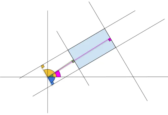
to standardize the input data and make extracting the interior of the film easier. Consider Fig. 2.14 in which the θ value for each line is represented by a colored, circular segment.
Figure 2.14: An illustration depicting the lines and their corresponding θ values, obtained from a Hough transform, for a MIP film.
Each normal line is colored, and its correspondingθ value is colored the same. Theθ
values can be used to find the rotation angle that levels the rectangle in this coordinate system. Through inspection, this rotation angle is
−1 4 4 X i=1 mod(θi,90) (2.19)
which is the negative of the average of each line’s angular distance to its closest axis (in the clock-wise direction). It is then added to each of the four lines’ θ value to set the lines so they become parallel to either the y or x axis. A built-in MATLAB function for rotating the actual images is used with this angle to rotate the actual image.
2.9
Edge Quality
The quality of the edge of a MIP film can be quantified in two ways: regularity, and strength. Edge regularity is a measure of how close the Canny edge is to the Hough transform line on average. If the Canny edge coincides perfectly with the line, it is perfectly regular. If it oscillates above and below, or runs parallel to the Hough transform line with a large separating distance, the Canny edge is considered very irregular. Edge strength is a measure of how many edge pixels exist in a given area of an image. In other words, it is a measure of edge pixel density. The more Canny edge pixels per unit of area, the higher the strength. Inversely, a low edge pixel density means the edge is weak for the area of the image under inspection. Both of these properties are calculated for segments of the sides of the MIP film to obtain local edge strength and regularity measures.
First, an area is defined for a given line segment on the Hough transform line of length L. For each line segment, a search area of length L and width W is formed, centered on the Hough transform line. The direction in which the length is defined is always parallel with the line segment under consideration. Edge regularity is obtained by calculating the average distance of the points in the Canny edge, within the search area, to the line found by the Hough transform. In this thesis,L= 0.8% of the image height, and W = 0.4% of the image width, which were approximately 30 and 20,
respectively. An example of a search area is shown in Fig. 2.15.
Figure 2.15: The lines obtained from the Hough transform are shown in green, the edge obtained from the Canny edge detector is shown in pink, and the search area to determine edge quality is shown in black.
The reasoning behind this step is that if there are any edge pixels that exist in close proximity to the Hough line but do not coincide with it, it must mean the edge is irregular and is therefore undesirable. Thus, a greater edge irregularity implies a lower quality MIP film. The height of the box is defined so that only pixels that are reasonably assumed to belong to the MIP film are chosen to calculate edge roughness. If the height is too large, then the algorithm will incorporate edge pixels from, say, the edge of the glass slide, which will result in a large average deviation from the Hough line, skewing the regularity measure. The regularity measure is defined as
E =
PN
i d(Pa, Pb,(xi, yi))
N (2.20)
which could equivalently be called “Mean Absolute Error,” where N is the number of edge points in the search area,Pa is the beginning point of the line segment of the Hough transform line,Pb is the endpoint of the line segment, (xi, yi) is the coordinates of the ith Canny edge pixel, and the functiond is given by
d(Pa, Pb,(x0, y0)) =
|(yb−ya)x0−(xb−xa)y0+xbya−ybxa|
p
(yb −ya)2+ (xb−xa)2
which gives the perpendicular distance of a Canny edge pixel to the line formed by
Pa and Pb.
Clearly, the more the Canny edge points deviate from the lines found from the Hough transform the higher the error will be. A line segment is classified as regular if it has an error of less than 0.15W. A line segment is classified as weak if it has fewer than LW40 Canny edge pixels. An example of a weak edge may also be seen in Fig. 2.15 at the top of the MIP film where there are evidently no Canny edge pixels.
2.10
Internal Angles
One property of interest for evaluating the quality of MIPs is the set of a MIP film’s internal angles. Depending on manufacturing feasibility and marketability, MIPs must be produced consistently with specific internal angles. Thus, internal angles should be used to assess quality. The angle of intersection between two sides is obtained through forming a vector from each line, by using the line’s endpoints, and calculat-ing the angle uscalculat-ing
φ= arccos u·v
kuk kvk (2.22)
whereu and v are the vectors corresponding to each of the two lines.
2.11
Threshold-Based Defect Detection
An additional simpler technique used to find defects is based on applying a high threshold to the images of the MIP films to form a black and white image, where the values of pixels are either one or zero, and calculating the total number of white pixels in the image. The premise is simple: due to the underlying white light shining through the glass slide any scrapes should appear in black and white images for high thresholds while all other pixels become suppressed, which can be seen in Fig. 2.16 and Fig. 2.17. The purpose of including this method is to compare its defect classification accuracy with the classification accuracy of the more complex SOM to determine the SOM’s feasibility as a defect detection algorithm.
Figure 2.16: A defective MIP film which has been isolated from its background.
2.12
Calculation of Feature Vector
Each image of a MIP film is divided into cells, and a feature vector is calculated for each cell. Each feature vector consists of features which describe their corresponding image cell. The raw feature vectors used for the data set are constructed from twenty different features. Features 1 and 2 are simple statistical measures, features 3-14 are Haralick texture features, and features 15-20 are custom features. The features used are as follows:
1. Mean gray Level 2. Median gray level 3. Angular second moment 4. Contrast
5. Variance
6. Inverse difference moment 7. Sum average 8. Sum variance 9. Sum entropy 10. Entropy 11. Difference variance 12. Difference entropy
13. Information measure of correlation II 14. Maximal correlation coefficient 15. Blob, threshold 0.5
16. Blob, threshold 0.6 17. Blob, threshold 0.7
18. Blob, threshold 0.8 19. Blob, threshold 0.9 20. Truth transition distance
2.12.1
Gray Levels
Mean gray level is calculated by first converting the image to a gray-scale image. In MATLAB, this is performed by calling “rgb2gray.” The intensity values, between 0 and 255, are then added to a running total for each pixel in the image and then averaged over the total number of pixels in the image. Similarly, the median gray level is calculated by finding the median intensity value for all pixels.
2.13
Haralick Texture Features
Image texture describes how the color/intensity levels in an image vary from pixel to pixel. According to Haralick [33][34], image texture is described by the number and types of so-called “tonal primitives” and the spatial organization of those primitives. Tonal primitives are maximally connected regions of an image which share the same tonal properties. A tonal property is described by gray tone properties, such as the highest or lowest gray level, and the tonal region properties, such as the shape or size. Thus, image texture is described by the number and types of its primitives and spatial organization of its primitives. Haralick captures the texture information from images composed of tonal primitives using the Haralick texture features.
2.13.1
Gray Level Co-Occurrence Matrix
The Haralick texture features describe the spatial inter-relationships of gray tones in textural patterns by making use of a so-called gray level co-occurrence matrix (GLCM). For each image cell in this thesis, the Haralick texture features are computed and therefore a GLCM is also computed for each cell. The GLCM can be specified by a matrix of relative frequenciesp. Each element of p,p(i, j), is the frequency at which a pixel with gray levelj occurred next to a pixel with gray leveliin a specified direction
and separated by distanced. GLCMs can be constructed by finding neighboring pixels in any direction; vertically, horizontally, diagonal, or a combination of the three. This co-occurrence approach characterizes the spatial distribution and spatial dependence among the gray tones in a local area. To elaborate on the meaning of the GLCM, consider the example image shown in Fig. 2.18. The GLCM for this image was created using an offset in the positivex-direction with a distance of one and is given by
p11 p12 p13 p14 p21 p22 p23 p24 p31 p32 p33 p34 p41 p42 p43 p44 = 1 1 0 0 0 3 2 0 0 0 2 0 0 1 1 1
Figure 2.18: A simple 4×4 image with 4 possible gray levels.
The GLCM can be made into a symmetric matrix by instead adding up the co-occurrence of pixel intensities in both positive and negative directions of the offset which generates the resulting GLCM of
2 1 0 0 1 6 2 1 0 2 4 1 0 1 1 2
Computing a symmetric GLCM assists in efficient computation of the Haralick texture features since it allows one to reduce the number of calculations by considering the
symmetry of the matrix. In this thesis, GLCMs are calculated by using an offset in the positive and negative x-direction with a distance of 1. Only this direction is used for speeding up processing since additional offsets require computing additional GLCMs and therefore increases computing time. However, it should be noted that one benefit of using multiple GLCMs is that it facilitates insensitivity to rotation or scale of the images.
The Haralick features are calculated as follows [35]. G is equal to 256, the number of gray levels used, and µis the mean of p.
Angular Second Moment (ASM) =X i X j p(i, j)2 (2.23) Contrast = G−1 X n=0 n2 G X i G X j p(i, j),|i−j|=n (2.24) Variance =X i X j (i−µ)2p(i, j) (2.25) Inverse difference moment (Homogeneity) =X
i X j 1 1 + (i−j)2p(i, j) (2.26) Sum average = 2G X i=2 ipx+y(i) (2.27) Sum entropy =− 2G X i=2 px+y(i) log (px+y(i)) =fs (2.28) Sum variance = 2G X i=2 (i−fs)2px+y(i) (2.29) Entropy =−X i X j p(i, j) log (p(i, j)) (2.30)
Difference Variance = Variance of px−y (2.31) Difference Entropy =− G−1 X i=0 px−y(i) log (px−y(i)) (2.32) Information measure of correlation II = (1−exp−2(HXY2−HXY))1/2 (2.33)
HXY =−X i X j p(i, j) log (px(i)py(j)) (2.34) HXY2 =−X i X j px(i)py(j) log (px(i)py(j)) (2.35) Maximal Correlation Coefficient = Square root of the second largest eigenvalue of Q (2.36) where Q(i, j) =X k p(i, k)p(j, k) px(i)py(k) (2.37) and px(i), py(j), px+y(i), andpx−y(i) are given by
px(i) = G X j=1 p(i, j) (2.38) py(j) = G X i=1 p(i, j) (2.39) px+y(k) = G X i=1 p(i, j), i+j =kandk = 2,3, ...,2G (2.40)
px−y(k) = G X i=1 G X j=1 p(i, j), i−j =k andk = 0,1, ..., G−1 (2.41)
px(i) is the sum of the ith row of p, and py(j) is the sum of the jth column of
p. These essentially give the number of times a pixel with intensity i (or j) occurred next to a pixel of any intensity. We refer the reader to the original paper by Haralick and coworkers [34] for an exposition on how to intuitively understand these texture features. Note that the correlation feature is not used in this thesis, since it becomes undefined for certain images.
2.14
Calculation of Intensity Resilience
The calculation of intensity resilience is a measure of how much the intensity of the image changes with respect to increasing threshold. An image with homogeneous, low gray levels will darken quickly with respect to an increasing threshold. An image with one or more bright spots will maintain such bright spots for higher thresholds than dimmer, homogeneous images. Here we introduce the concept of intensity transition distance, later called “truth transition distance” (TTD).
Figure 2.19: An example of a MIP film with two regions of different texture which is highlighted.
Consider Fig. 2.19. Two regions are highlighted: the one on the left containing light speckles and the other containing a very visible scratch in which the underlying
Figure 2.20: An binary image of the MIP film shown in Fig. 2.19
illuminated glass slide is visible. The image is converted to a black and white binary image shown in Fig. 2.20.
Figure 2.21: Plots, and their corresponding image cells, which show how the total fraction of the image that is white decreases with respect to increasing threshold.
In Fig. 2.21, the lower left image is a closeup of the prominent scratch in Fig. 2.19 while the lower right image is a closeup of the speckled region. The plots above are the total fraction of the highlighted image sections that are made up of white pixels with respect to increasing threshold. For each threshold value, the image is converted to a black and white image with the threshold applied. For the scratched regions, the fraction of white pixels, or “truth” as we call it, remains higher for higher thresholds compared to speckled regions. This brings us to the concept of “truth transition distance,” or how long it takes for an intensity image to completely darken with respect to increasing threshold. According to Fig. 2.21, this quantity, which is just the arc length of the curve for truth values greater than 0.0001, can therefore be used to differentiate bright scratches from dull, dimly lit, or speckled regions. Additionally, the features referred to as “blob” are calculated by finding the largest maximally-connected group of white pixels within the image cell for a given threshold, calculating its size, and normalizing it by the surface area of the image cell it is contained within. For example, “blob 0.5” finds the blob value at threshold=0.5.
2.15
Principal Component Analysis
PCA is an orthogonal linear transformation which maps a set of vectors defined in some space to a new space spanned by orthogonal basis vectors such that the greatest variance of the transformed data set occurs along the first basis vector, and the second greatest variance of the data occurs along the second, and so on [36]. Consider Fig. 2.22.
Figure 2.22: A two-dimensional data set plotted with respect to its two feature vari-ables.
Variable x1 is clearly highly correlated with variable x2. Upon observation, it is
also clear that there seems to be a single direction in which the data vary the most. This direction can be obtained using PCA, which will take ann-dimensional data set ofm observations and returnnprincipal component vectors. In this case, sincen = 2, there will be two principal component vectors.
Figure 2.23: A two-dimensional data set projected into a space spanned by its two principal component vectors.
In Fig. 2.23, there is arguably just one principal component needed to “retain” most of the variance in the original data set. Thus, the second principal component
vector may be discarded and the data set is reduced in dimensionality from two dimensions to one.
The data set, which can be defined as Y, is mathematically defined as a matrix withn rows and m columns; each observation corresponds to a row and each column corresponds to the value of a feature for that observation. Y is z-scored to form X, meaning that each column of X is scaled by subtracting from it its mean and then dividing it by its standard deviation. This ensures all data points are on the same scale.
The mathematical transformation of X is performed by constructing vectors
w(k) = (w1, ..., wm)(k) (2.42)
fork=1, ...,l where l is the maximum number of principal components chosen. Each component of w(k) is simply a weight which determines how much of each of the
originalm basis vectors influences the resulting basis vectors. Each new basis vector is a linear combination of the original m basis vectors that is weighted such that the variance is maximized along the new basis vector while still being orthogonal all other principal component vectors. The first weight vectorw(1) is defined as
w(1) = arg max kwk=1 ( X i (t1)2(i) ) = arg max kwk=1 ( X i x(i)·w 2 ) (2.43)
wherex(i) is a row ofX and the dot productx(i)·wcalculates the so-called principal
component score for each data point
tk(i)=x(i)·w(k) for i= 1, . . . , n k = 1, . . . , l (2.44)
The summation is maximized when the spread of the data along w is maximal. Eqn. 2.43 can be rewritten in a form that involves the Rayleigh quotient.
w(1) = arg max kwk=1 {kXwk2}= arg max kwk=1 wTXTXw (2.45) which is equivalent to
w(1) = arg max wTXTXw wTw (2.46)
sincewis constrained to be a unit vector. XTXhappens to be a positive semi-definite matrix, and a standard solution is that the Rayleigh quotient is maximized when w is parallel with the eigenvector of the matrix. The maximal value for the Rayleigh quotient is the corresponding eigenvalue. The kth principal component is found by subtracting the first k −1 principal components from the data set given by X and then finding the unit vector which has the highest principal component score on the resulting data set,
ˆ Xk =X− k−1 X s=1 Xw(s)w(Ts) (2.47) w(k) = arg max kwk=1 n kXˆkwk2 o = arg maxnwTXˆTkXˆkw wTw o . (2.48)
Finally, the resulting transformed data set is given by
T=XW (2.49)
whereWis ap×pmatrix with rows being the weight vectors for each principal com-ponent in order of principal comcom-ponent number. Dimension reduction can then be performed by considering the eigenvalue corresponding to each principal component, and ignoring all but the firstm−L principal components to give
TL=XWL (2.50)
2.16
Self Organizing Map
A self organizing map (SOM) uses the idea of competitive learning that is inspired by processes that occur in complex biological systems such as the brain [37]. The topological organization of the brain is such that specific areas are stimulated by specific inputs more than others, forming a type of “map” with regions that could be associated with cognitive phenomena such as smell, memories, or joy. For example, the region of the brain associated with visual perception has maps for line orientation and color. This spatial organization of internal representations of information in the brain is what inspired a similar type of artificial learning system: the self organizing map.
2.16.1
Competitive Learning
Competitive learning first requires a set of statistical samples of a vectorial observable
x=x(t)∈Rn (2.51)
wherex(t) indicates the vector at iteration t. In addition to the samples, or training data, there are the reference vectors given by
mi(t) =mi ∈Rn, i= 1,2, ..., k. (2.52) Each reference vector is initialized randomly. Each of the k reference vectors are compared with the current training vector under consideration. Once the reference vector that is closest to the training vector is found, it is updated by some operation such that it becomes more aligned with the training vector. For example, the Eu-clidean distance is used as the criterion for determining the best matching reference vector. The result of repeating this process for a sufficient number of iterations is that eventually the reference vectors tend to point towards the points in space with the highest density of training vectors, and thus will approximate the underlying proba-bility distribution. One such example of a method which produces an approximation to a continuous probability density function ρ(x) of the vectorial input variable x is