David O. Davis
Glenn Research Center, Cleveland, Ohio
CFD Validation Experiment of a Mach 2.5
Axisymmetric Shock-Wave/Boundary-Layer
Interaction
NASA/TM—2015-218841
AJK2015–06342
NASA STI Program . . . in Pro
fi
le
Since its founding, NASA has been dedicated to the advancement of aeronautics and space science. The NASA Scientifi c and Technical Information (STI) Program plays a key part in helping NASA maintain this important role.
The NASA STI Program operates under the auspices of the Agency Chief Information Offi cer. It collects, organizes, provides for archiving, and disseminates NASA’s STI. The NASA STI Program provides access to the NASA Technical Report Server—Registered (NTRS Reg) and NASA Technical Report Server— Public (NTRS) thus providing one of the largest collections of aeronautical and space science STI in the world. Results are published in both non-NASA channels and by NASA in the NASA STI Report Series, which includes the following report types:
• TECHNICAL PUBLICATION. Reports of
completed research or a major signifi cant phase of research that present the results of NASA programs and include extensive data or theoretical analysis. Includes compilations of signifi cant scientifi c and technical data and information deemed to be of continuing reference value. NASA counter-part of peer-reviewed formal professional papers, but has less stringent limitations on manuscript length and extent of graphic presentations.
• TECHNICAL MEMORANDUM. Scientifi c
and technical fi ndings that are preliminary or of specialized interest, e.g., “quick-release” reports, working papers, and bibliographies that contain minimal annotation. Does not contain extensive analysis.
• CONTRACTOR REPORT. Scientifi c and
technical fi ndings by NASA-sponsored contractors and grantees.
• CONFERENCE PUBLICATION. Collected
papers from scientifi c and technical conferences, symposia, seminars, or other meetings sponsored or co-sponsored by NASA. • SPECIAL PUBLICATION. Scientifi c,
technical, or historical information from NASA programs, projects, and missions, often concerned with subjects having substantial public interest.
• TECHNICAL TRANSLATION.
English-language translations of foreign scientifi c and technical material pertinent to NASA’s mission. For more information about the NASA STI
program, see the following:
• Access the NASA STI program home page at
http://www.sti.nasa.gov
• E-mail your question to help@sti.nasa.gov • Fax your question to the NASA STI
Information Desk at 757-864-6500
• Telephone the NASA STI Information Desk at 757-864-9658
• Write to:
NASA STI Program Mail Stop 148
NASA Langley Research Center
David O. Davis
Glenn Research Center, Cleveland, Ohio
CFD Validation Experiment of a Mach 2.5
Axisymmetric Shock-Wave/Boundary-Layer
Interaction
NASA/TM—2015-218841
AJK2015–06342
National Aeronautics and
Space Administration
Glenn Research Center
Cleveland, Ohio 44135
Prepared for the
Joint Fluids Engineering Conference 2015
cosponsored by ASME, JSME, and KSME
Seoul, Korea, July 26–31, 2015
Available from
Trade names and trademarks are used in this report for identifi cation only. Their usage does not constitute an offi cial endorsement,
either expressed or implied, by the National Aeronautics and Space Administration.
Level of Review: This material has been technically reviewed by technical management. This report is a formal draft or working
paper, intended to solicit comments and ideas from a technical peer group.
This report contains preliminary fi ndings, subject to revision as analysis proceeds.
NASA STI Program Mail Stop 148
NASA Langley Research Center Hampton, VA 23681-2199
National Technical Information Service 5285 Port Royal Road Springfi eld, VA 22161 703-605-6000
Acknowledgments
Funding from the Transformational Tools and Technologies Project of the NASA Transformative Aeronautics Concepts Program is gratefully acknowledged. This work was sponsored by the Transformative Aeronautics Concepts Program at the NASA Glenn Research Center.
CFD Validation Experiment of a Mach 2.5 Axisymmetric
Shock-Wave/Boundary-Layer Interaction
David O. Davis
National Aeronautics and Space Administration Glenn Research Center
Cleveland, Ohio 44135
Abstract
Preliminary results of an experimental investigation of a Mach 2.5 two-dimensional axisymmetric shock-wave/ boundary-layer interaction (SWBLI) are presented. The purpose of the investigation is to create a SWBLI dataset specifically for CFD validation purposes. Presented herein are the details of the facility and preliminary measurements characterizing the facility and interaction region. These results will serve to define the region of interest where more detailed mean and turbulence measurements will be made.
Introduction
Experimental investigations of specific flow phenomena can provide great insight into the flow behavior but often lack the necessary detail and documentation to be useful as CFD validation experiments. Reasons for this include, but are not limited to:
• Undefined boundary conditions
• Inconsistent results
• Undocumented 3D effects (centerline only measurements)
• Lack of uncertainty analysis
In 1994, Settles and Dodson (Refs. 1 and 2) reviewed a large number of supersonic and hypersonic experiments and evaluated them for suitability to be used as CFD validation experiments. Of the hundreds of experiments reported in the open literature, over one hundred were subjected to rigorous acceptance criteria. Of these, only nineteen (12 supersonic, 7 hypersonic) were deemed to be acceptable for CFD validation. Aeschliman and Oberkampf (Ref. 3) recognized the need to develop a specific methodology for experimental studies intended specifically for validation purposes.
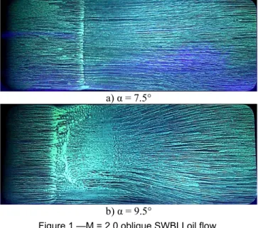
SWBLI CFD validation experiments performed in non-circular wind tunnels pose a particularly challenging problem, as streamwise and transverse pressure gradients induced by the SWBLI turn a nominally two-dimensional flow-field into a three-dimensional flow-flow-field (Refs. 4 and 5). This is illustrated in Figure 1 by oil flow visualization obtained in NASA Glenn Research Center’s (GRC) 15×15 cm Supersonic Wind Tunnel (SWT) with an M = 2.0 oblique SWBLI.
The view is of the floor of the tunnel where an impinging/ reflected oblique shock wave interacts with the boundary layers on the floor and sidewalls and α is the angle of the shock
generator plate. For a weak, unseparated interaction (Figure 1(a)), the flow remains mostly two-dimensional with a slight bottlenecking of the limiting wall streamlines in the vicinity of the impingement location. For a stronger, separated interaction, (Figure 1(b)), centerline measurements alone would not be representative of a two-dimensional interaction and the entire flow-field would need to be surveyed for this case to be useful as a CFD validation case.
The Transformational Tools & Technologies (TTT) Project under NASA’s Transformative Aeronautics Concepts Program is tasked, in part, with providing quality experiments for the purpose of validating CFD codes and turbulence models. A Mach 2.5 SWBLI has been identified as one of the test cases desired. The primary objective of the current study is to provide a comprehensive dataset for a Mach 2.5 SWBLI that is of sufficient quality to be used as a validation test case.
In order to avoid the pitfalls of a rectangular configuration, an axisymmetric configuration is proposed that is two-dimensional in the mean. The selected interaction is illustrated in Figure 2. A Mach 2.5 core flow approaches a cone-cylinder centerbody that generates a conical shock that impinges and reflects off the cylindrical test section wall, interacting with the naturally occurring test section boundary layer. The approximate measurement area of interest is indicated by the rectangular box shown in the figure. NASA GRC’s supersonic facilities, however, all have square or rectangular test sections so a new facility has been designed specifically for this study. This configuration is similar to a study performed by Rose (Ref. 6), which was considered for Settles and Dodson’s validation database, but was rejected due to questions about the accuracy of the hot-wire measurements. A new 17 cm diameter axisymmetric supersonic wind tunnel (Axi-SWT) has been installed in Test Cell W6B and replaces the existing 15×15 cm configuration. The facility design allows for relatively easy changes between the square and circular configurations.
The goal of the initial characterization is to define the interaction region of interest where more refined and redundant measurements will be taken. These measurements will include hot-wire data to quantify the turbulence structure through the interaction region.
a) α = 7.5°
b) α = 9.5°
Figure 1.—M = 2.0 oblique SWBLI oil flow.
Figure 2.—M = 2.5 Axisymmetric SWBLI. (box indicates region of interest).
Nomenclature
A Area
CD Discharge coefficient
Cf Skin friction coefficient
CL Centerline D Diameter
gc Proportionality constant
Hi Incompressible boundary-layer shape factor
Lt ASME bellmouth throat length (Figure 5)
M Mach number
N Number of redundant measurements (Table 1) p Pressure
R Radius
R1 ASME nozzle ellipse major radius (Figure 5) R2 ASME nozzle ellipse minor radius (Figure 5) Rc Radius of curvature
Rair Gas constant for air
ReD Reynolds number based on diameter
ReDs Scaled Reynolds number (ReDs = ReD× 10E-06)
T Temperature or throat tap location (cm, Figure 5) U Velocity
w Mass flow rate
xsup Axial coordinate relative to C-D nozzle throat (Figure 6)
x,y,z Cartesian coordinates x,r,θ Cylindrical coordinates Greek Symbols
α Shock generator cone half-angle (deg)
β Ratio of ASME nozzle-to-approach pipe diameter
γ Ratio of specific heats for air (1.4) δ Boundary-layer thickness
δ* Boundary-layer displacement thickness
δXi Uncertainty of measureand Xi
θ Boundary-layer momentum thickness
μ Molecular viscosity
ρ Density Subscripts
0 Pertaining to plenum conditions bm Pertaining to the ASME bellmouth
e Pertaining to boundary-layer edge condition i Pertaining to ideal conditions
noz Pertaining to the C-D nozzle t Pertaining to total conditions th Pertaining to throat conditions ts Pertaining to the test section w Pertaining to wall conditions
Axisymmetric SWBLI
As previously mentioned, an axially symmetric SWBLI is the only practical way to ensure a two-dimensional flow in the mean. A number of axisymmetric SWBLIs have been investigated over the years. These include supersonic flow over a double-cone, over a cylinder-flare, an impinging-centerbody SWBLI, and the present configuration of an impinging-duct SWBLI as shown in Figure 3.
The impinging duct configuration was chosen for two reasons. First, inasmuch as the intent of the investigation is to provide CFD validation data, this configuration allows for a relatively thick incoming boundary layer so highly resolved
Figure 3.—Axisymmetric SWBLI configurations. measurements are possible. And second, although not intended to mimic any particular application, it is of the same general configuration as a SWBLI occurring on the cowl surface of axisymmetric inlets with supersonic internal compression. Previous investigations of this flow configuration include the development of integral flow models for solid and porous walls by Seebaugh et al. (Ref. 7). An experimental investigation by Seebaugh and Childs (Ref. 8) presented surface static and flowfield Pitot pressure measurements under Mach 2.82 and 3.78 flow conditions with cone angles of 10°, 13°,and 15°. Rose (Ref. 6) acquired detailed turbulence measurements using hot-wire anemometry under Mach 3.88 flow conditions with a
9° cone angle. Neither of the latter two studies, however, were
considered to meet the criteria for CFD validation purposes as proposed by Reference 1.
Facility Description
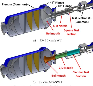
The new 17 cm axisymmetric facility is located in Test Cell W6B at NASA GRC. W6B is a continuous flow supersonic facility with Mach number variation achieved by interchangeable fixed-geometry nozzle blocks. The plenum chamber is supplied with dry ambient temperature compressed air up to 377 kPa. The exhaust side of the tunnel is connected to lab-wide altitude exhaust which is maintained at less than 13.8 kPa. The 17 cm Axi-SWT utilizes the same plenum chamber and exhaust as NASA GRC’s 15×15 cm SWT. A test section diameter of 17 cm was selected so as to maintain similar flow area as the 15×15 cm SWT. Figure 4 shows a section view of both facilities.
With reference to Figure 4(a), installation of the 15×15 cm SWT bellmouth requires removal of the 44 in. flanged bulkhead on the plenum chamber. To allow the facility to be reconfigured between the two configurations with a minimum of effort, the bellmouth for the 17 cm Axi-SWT was designed so as to only require removal of the 18 in. interface flange. A new bellmouth for the 15×15 cm SWT is currently in the design cycle to allow similar installation.
As illustrated in Figure 4(b), the 17 cm Axi-SWT required design and fabrication of three major components: the bellmouth, the convergent-divergent (C-D) supersonic nozzle,
a) 15×15 cm SWT
b) 17 cm Axi-SWT
Figure 4.—Section view of W6B test facility.
and the test section. Beyond these basic components for the facility, the Shock Generator (SG) hardware is also required. A brief description of each component follows.
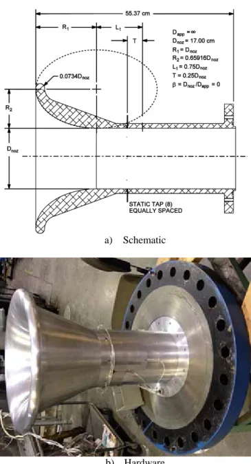
ASME Bellmouth
The bellmouth for the axisymmetric facility serves two purposes. First, it is used to provide a uniform, low Mach number flow to the C-D nozzle, and second, it is used to measure the total mass-flow through the facility:
i noz bm D noz C w w = , ⋅ , (1)
where wnoz,iis the ideal mass-flow given by:
) 1 ( 2 ) 1 ( 2 0 , 0 , , 1 21 ⋅γ− + γ − γ− ⋅ + ⋅ ⋅ ⋅ ⋅ ⋅ γ = noz t noz noz t air c i noz Rg p MT A M w (2) Geometry
The elliptical bellmouth geometry is based on an ASME Long-Radius Flow Nozzle with throat taps and is a scaled version of similar bellmouths used at NASA GRC. A schematic of the bellmouth and a photo of the actual hardware are shown in Figure 5(a) and Figure 5(b), respectively. This design conforms to the Low-β Nozzle with Throat Taps illustrated in Figure II-III-14 of Reference 9 with the following two exceptions. First, no approach pipe exists before the nozzle (Dapp = ∞), hence β =
Dnoz/Dapp=0. And second, the nozzle exit flow does not exhaust
into a sudden expansion but rather a constant area diffuser.
a) Double-Cone b) Cylinder-Flare
c) Impinging-Centerbody d) Impinging-Duct
Plenum (Common) 44” Flange18” Flange
Test Section #3 (Common) Bellmouth C-D Nozzle Square Test Section Bellmouth C-D Nozzle Circular Test Section
a) Schematic
b) Hardware
Figure 5.—ASME bellmouth. ASME Nozzle Discharge Coefficient
The discharge coefficient for the bellmouth was determined from a computational calibration performed on a geometrically similar nozzle. The details of the calibration are given in Reference 10.
M f C CD,bm D,M0.5 (3) where bm D M D C , 5 . 0 , Re 73896 . 6 993003 . 0 (4) and
1-0.2 2
0.00863415 0.999514 ) (M Mbm f (5) and bm bm bm bm bm D D U , Re (6)For the current M = 2.5 C-D nozzle, the ratio of bellmouth
throat area to nozzle throat area (Abm,th/Anoz,th) is 2.636, so the
Mach number in the ASME bellmouth will be approximately Mbm,th = 0.21.
C-D Nozzle
A schematic of the C-D nozzle is shown in Figure 6. The requirements for the C-D nozzle design include:
1) Exit Mach number of 2.5
2) Inlet and exit diameter equal (17 cm)
3) Length approximately the same as 1515 cm nozzles
(~66 cm)
The second requirement allows for the C-D nozzle to be replaced with a constant area duct so that the facility can also be run subsonically.
The steps for designing the nozzle include:
1) Definition of the inviscid, shock-free supersonic contour.
2) Definition of the subsonic contour (contraction).
3) Correction of the supersonic contour for B.L. growth.
4) Adjustment of the subsonic contour.
For the first step a Method of Characteristics (MOC) approach was used. To define the inviscid supersonic contour, the exit
Mach number, the radius of curvature at the throat (Rc,th), and a
function for the initial expansion are required. To minimize
distortion of the sonic line at the throat, Rc,th should be large.
But as Rc,th is increased, the correction for boundary-layer
growth becomes more significant and the nozzle length is
increased, thus a balance must be achieved. For the current nozzle, given the length constraints, Rc,th was selected as:
th th
c R
R , =8.0⋅ (7)
where Rth is the nozzle radius at the throat. For the initial
expansion, a parabolic function was chosen: 2 sup , 2 0 . 1 ⋅ ⋅ + = th th c th th R x R R R r (8)
where xsup is the axial coordinate with origin at the inviscid
nozzle throat.
For the subsonic contour, the parabolic function for the initial supersonic contour was extended upstream to an arbitrary point. Then a 5th order polynomial function was specified to transition from the upstream constant area section to the parabolic section. A 5th order polynomial allows for continuous second derivatives of the contour.
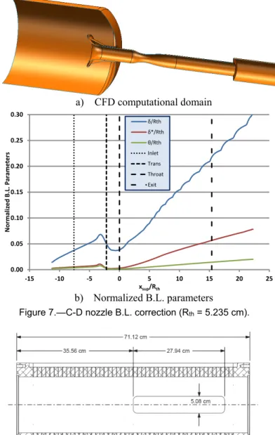
There are a number of methods available to correct for the boundary-layer growth in a nozzle. The most common is to correct the contour by an estimate of the displacement thickness growth through the nozzle. For this nozzle, we chose to estimate the displacement thickness growth by performing a numerical simulation using the Wind-US flow solver (Ref. 11) in conjunction with the Menter Shear Stress Transport (SST) turbulence model (Ref. 12). With reference to Figure 7(a), the computational domain included the plenum tank, ASME bellmouth, C-D nozzle, test section and dump diffuser. The resulting boundary-layer parameter variations through the facility are shown in Figure 7(b).1
In this figure, the line labelled “Trans” is the location where the contour transitions from the 5th order polynomial function to the parabolic function. Between this location and the nozzle exit, the displacement thickness distribution was fit with a 6th order polynomial and the nozzle contour was adjusted for displacement thickness growth. The final step was to reevaluate the 5th order polynomial coefficients to account for the adjusted downstream contour.
Test Section
The test section is basically a constant area cylinder. Two test sections have been fabricated. The first is instrumented with wall static taps and two opposing windows as shown in Figure 8. The primary purpose of the windows is to allow access for probe setup and alignment of the shock generator centerbody. These windows will also be used to evaluate a dynamic skin friction film measurement technique.
1The waves in the boundary-layer thickness (δ) are an artifact of the algorithm used to locate the boundary-layer edge.
a) CFD computational domain
b) Normalized B.L. parameters
Figure 7.—C-D nozzle B.L. correction (Rth = 5.235 cm).
Figure 8.—Test section schematic.
The second blank test section is a plain cylinder with provisions to mount the end flanges. This section will be modified at a later date to include optical access for a Particle Image Velocimetry (PIV) system that is currently being designed. A photo of the C-D nozzle and test section are shown in Figure 9. Currently the windows in the test section are aluminum blanks which will be modified to accept additional instrumentation once the extent of the interaction region has been defined. The interior surface of the window is contoured to conform with the circular test section.
0.00 0.05 0.10 0.15 0.20 0.25 0.30 -15 -10 -5 0 5 10 15 20 25 N or ma liz ed B .L. P ar ame ter s xsup/Rth δ/Rth δ*/Rth θ/Rth Inlet Trans Throat Exit
Figure 9.—C-D nozzle and test section.
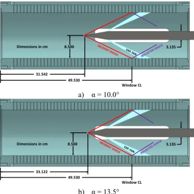
Shock Generator
The shock generator (SG) is a cone-cylinder located on the centerline of the wind tunnel as shown in Figure 10. The investigation will initially focus on two SG configurations. Both have a cylinder diameter of 3.135 cm, however, the cone angles differ with one having a half-angle of 10.0° and the other
having a half-angle of 13.5°. The former is expected to generate a relatively weak interaction, while the latter will generate a stronger interaction with the possibility of creating boundary-layer separation. The axial placement of the cone tip was chosen so that the conical shock generated by the cone impinges at approximately the center of the window. The window is placed in the downstream half of the test section to minimize the length of the cantilevered SG and also to allow for maximum boundary-layer development.
The centerbody diameter was chosen to minimize blockage of the cantilevered probe configuration. The concern was that in the vicinity of the interaction, the presence of the probe support might cause a local unstart of the wind tunnel. The relatively small centerbody diameter, however, causes close-coupling of the shock-wave and expansion which results in a rapid pressure rise and fall. Once these two baseline interactions are documented, a larger centerbody will be considered as a future test case.
The SG is cantilevered from the end of the test section as show in Figure 11. For the initial measurements, the cone configuration is changed by replacing the entire cone-cylinder. A cylinder with removable tips is currently being designed to allow changing the cone configuration without requiring realignment of the cylinder.
Instrumentation
For the initial characterization of the interaction regions, conventional pressure instrumentation is used. This consists primarily of wall static pressure taps and Pitot probes for flowfield measurements. Figure 12 shows the general layout of this instrumentation. The throat of the ASME bellmouth has eight equally spaced static pressure taps. Similarly, the C-D nozzle also has eight equally spaced static pressure taps located near the exit plane.
a) α = 10.0°
b) α = 13.5°
Figure 10.—Shock generator schematic.
Figure 11.—Shock generator assembly.
Figure 12.—Pressure instrumentation.
Window CL 3.135 31.542 49.530 8.500 Dimensions in cm Window CL 3.135 49.530 8.500 33.122 Dimensions in cm Bellmouth (8) Test Section (156) Press. Probe (12) C-D Nozzle (8) Exhaust (6) Test Section #3
Figure 13.—Test section static pressure taps.
These taps are located 2.54 cm downstream from the end of the nozzle contour and 3.81 cm upstream of the start of the test section (x = 0 plane).
The test section has 156 static pressure taps laid out as shown in Figure 13. The first tap for all the stations begins 5.08 cm downstream from the test section inlet plane. Along the top (AA) and bottom (BB), there are 49 equally spaced taps. Along CP and CS there are 23 equally spaced taps. The axial spacing for the taps along AA, BB, CP, and CS are 1.28 cm. There are three equally spaced taps along DP, DS, EP, and ES. The axial spacing at these stations is 35.56 cm.
With reference to Figure 12, the flow from the circular test section dumps into what is referred to as Test Section #3 which is a 25.4×25.4 cm square section. Up to six base pressures can be measured where the flow from the circular test section exits as a free-jet into the square section. Test Section #3 also has a probe traversing capability. Plates on the top and bottom of this section translate in the traverse horizontal direction. An actuator that can be mounted on either the top or bottom plate allows a probe to be translated in the vertical direction. Thus, the combination of these allows a probe to be located anywhere within the test section cross-plane. Both the horizontal and vertical directions are driven by remotely actuated stepper motors. The position of each axis is measured with digital encoders. Currently, positioning the probe in the axial direction is a manual operation.
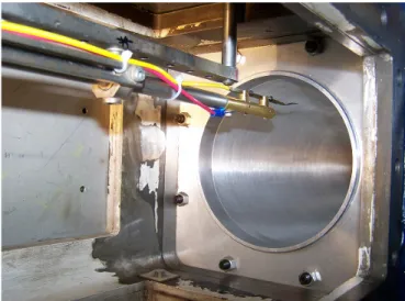
In addition to surveying in the axisymmetric test section, the facility can also be configured to survey the exit plane of the C-D nozzle. An interior photo of Test Section #3 showing a probe setup for a boundary-layer survey at the C-D nozzle exit is shown in Figure 14. The nose of the probe sting is electrically isolated from the support rod using a nylon threaded rod and washer. This allows probe wall touch to be established by electrical continuity.
In addition to the aforementioned instrumentation, total temperature and total pressure in the plenum chamber are also recorded. Inasmuch as the total temperature is at ambient conditions and can drift over time, the facility controls are setup to automatically adjust the plenum total pressure to maintain a constant Reynolds number.
Figure 14.—C-D nozzle exit plane survey.
TABLE 1.—MEASURAND UNCERTAINTY
Uncertainty Considerations
A detailed uncertainty analysis is still in progress but the measurand uncertainties have been estimated and are summarized in Table 1. These uncertainties include the sensor uncertainty as well as the uncertainty associated with the signal processing in the data acquisition system (Ref. 13). The variable N represents the number of redundant transducers associated with a measurand. These uncertainties will be combined with estimates of the probe (static tap and Pitot probe) measurement uncertainties which will then be propagated through the calculation procedures. AA BB CS CP ES DS EP DP
VIEW LOOKING UPSTREAM VIEW AA-BB
AA1 AA25 AA49
BB1 BB25 BB49
EP1 EP25 EP49
DP1 DP25 DP49
CP1 CP23
FLOW 5.08 cm
i Description Xi δXi Ν δXi Units
1 Plenum total temp. Tt,0 1.39 2 0.982 °K
2 Plenum total pressure pt,0 0.0689 1 0.0689 kPa
3 Bellmouth throat static pressure pbm 0.0255 8 0.0090 kPa
4 Bellmouth throat diameter Dbm 0.0013 1 0.0013 cm
5 Bellmouth discharge coefficient CD,bm 0.0025 1 0.0025
-6 C-D nozzle exit plane static pressure pnoz 0.0621 8 0.0219 kPa
7 Probe position, x xprb 0.0064 1 0.0064 cm
8 Probe position, y yprb 0.0064 1 0.0064 cm
9 Probe position, z zprb 0.0064 1 0.0064 cm
Results and Discussion
ASME Bellmouth and C-D Nozzle Condition
The facility was initially setup to survey the C-D nozzle exit plane as shown in Figure 14. Prior to performing the surveys, the nozzle Mach number was measured. The Mach number was calculated from the isentropic relation:
− ⋅ − γ = γ − γ 1 1 2 ,0 1 noz t noz pp M (9)
where pt,0 is the plenum total pressure and pnoz is the average of
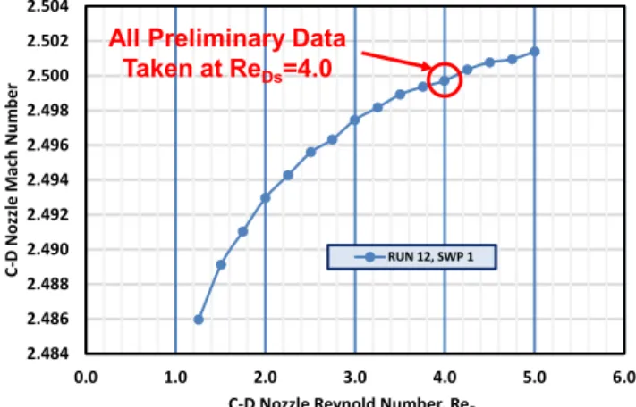
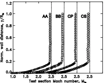
the eight static pressures located at near the nozzle exit. The C-D nozzle exit plane Mach number as a function Reynolds number is shown in Figure 15. The uncertainty in the Mach number measurement based on values in Table 1, which excludes the pressure tap uncertainty, is estimated to be less than 0.05 percent over the Reynolds number range plotted. The design Mach number of 2.5 is achieved at a Reynolds number of approximately 4.0E+06. This Reynolds number was subsequently selected as the operating point for the characterization of the facility.
The mass-flow through the facility was measured with the ASME bellmouth by the method described in Reference 10. The mass-flow as a function C-D nozzle Reynolds number is shown in Figure 16. The uncertainty in the mass-flow measurement based on values in Table 1, which excludes the pressure tap uncertainty, is estimated to be less than 0.4 percent over the Reynolds number range plotted. The mass flow at
ReD,noz = 4.0E+06 is approximately 4.7 kg/s.
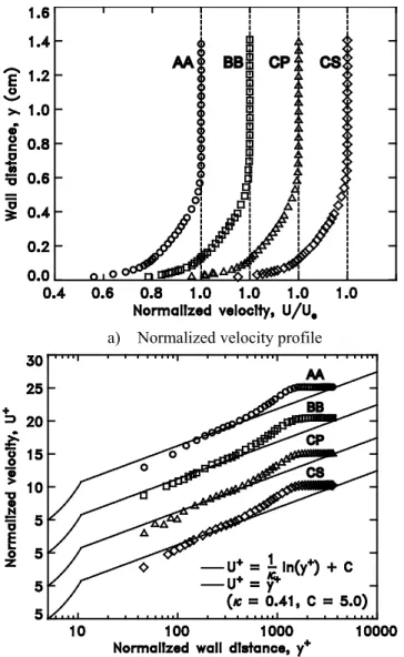
With reference to Figure 13, Pitot pressure surveys were taken along vertical (AA, BB) and horizontal (CP, CS) planes. These surveys, plotted in terms of Mach number, are shown in Figure 17. From this plot, the core profile is seen to be quite uniform with good agreement with the bulk Mach number from Figure 15. The largest deviation in Mach number occurs near the centerline which is somewhat typical of C-D nozzles.
The boundary-layer region of the profiles shown in Figure 17 was analyzed to calculate relevant boundary-layer parameters. The boundary-layer profiles plotted in terms of velocity normalized by the boundary-layer edge velocity and in terms of van Driest (Ref. 14) scaled variables are shown in Figure 18(a) and Figure 18(b), respectively. With reference to Figure 18(b), the profiles generally follow the law-of-the-wall, but perhaps with a slightly elevated slope which is likely a result of distortion by the strong favorably pressure gradient in the nozzle. The average boundary-layer parameters from the four profiles are summarized in Table 2 (EXP, x = –3.81 cm). Also shown in this table for comparison are the results of the Wind CFD analysis (WIND, x = –3.81) used to correct the nozzle contour. Note that this is an approximate comparison since the Wind results were for the inviscid nozzle contour which results in a slightly lower Mach number.
Figure 15.—C-D nozzle bulk Mach number.
Figure 16.—17 cm Axi-SWT mass flow.
Figure 17.—Mach number at C-D nozzle exit, ReDs,noz = 4.0. 2.484 2.486 2.488 2.490 2.492 2.494 2.496 2.498 2.500 2.502 2.504 0.0 1.0 2.0 3.0 4.0 5.0 6.0 C-D N ozzl e M ac h N um be r
C-D Nozzle Reynold Number, ReDs RUN 12, SWP 1
All Preliminary Data Taken at ReDs=4.0 y = 1.176x - 0.039 R² = 1.000 0.0 1.0 2.0 3.0 4.0 5.0 6.0 7.0 0.0 1.0 2.0 3.0 4.0 5.0 6.0 Mas s-flow , w (k g/ s)
C-D Nozzle Reynold Number, ReDs RUN 12, SWP 1 Linear (RUN 12, SWP 1)
a) Normalized velocity profile
b) Law-of-the-wall
Figure 18.—Boundary-layer profiles at C-D nozzle exit.
Figure 19.—Wall pressure distribution through test section.
2For clarity, the distributions s are shifted by Pw/Pt,0 = 0.01.
TABLE 2.—BOUNDARY-LAYER PARAMETERS
The measured boundary-layer thickness at the nozzle exit is approximately 0.61 cm, which is somewhat thinner than the results of the Wind analysis (0.69 cm). The integral properties, however, are in quite good agreement. The incompressible shape factor at the nozzle exit, which is typically about 1.3 for a fully turbulent, zero pressure gradient boundary layer, is slightly elevated and likely a result of the transition from strong favorable pressure gradient to mild adverse pressure gradient at the nozzle exit.
Shock-Free Flow Through Test Section
After completion of the preliminary measurements of the nozzle, the facility was reconfigured with the test section as shown in Figure 4(b). Without a shock generator, the flow through the test section is supersonic developing pipe flow with friction, or Fanno line flow.
Wall static pressure distributions at a Reynolds number of
ReDs,noz = 4.0 are show in Figure 19.2 As expected, the pressure
rises slightly through the test section. There is observed to be some slight scatter in the data and also slight differences between the upper (AA) and lower (BB) distributions in the second half of the test section. This will be investigated further by checking alignment with the nozzle and also by rotating the
test section 180° and repeating the measurements. In fact, one
aspect of this investigation will be to document and quantify the sensitivity of the results to tunnel assembly procedure and configuration.
With reference to Figure 13, Pitot pressure surveys were taken along vertical (AA, BB) and horizontal (CP, CS) planes at the last static pressure tap location (x = 66.0 cm) at a scaled Reynolds number of ReDs,noz = 4.0. These surveys, plotted in
terms of Mach number, are shown in Figure 20. At this station the Mach number in the core has dropped to about 2.4. The profiles at CP and CS show a slightly higher than core point at the edge of the boundary layer which is absent from the profiles at AA and BB. This has been traced to a small forward facing step at the downstream end of the window. The windows are currently being modified to eliminate this step.
The boundary-layer profiles at the test section exit plotted in terms of velocity normalized by the boundary-layer edge velocity and in terms of van Driest (Ref. 14) scaled variables are shown in Figure 21(a) and Figure 21(b), respectively. The average boundary-layer parameters at the test section are summarized in Table 2. The edge Mach number is reduced to
0.04 0.05 0.06 0.07 0.08 0.09 0.10 0.11 0.12 0.13 0.14 0 10 20 30 40 50 60 70 pw /pt,0 x (cm) AA BB CP CS DP DS EP ES 0.06 0.06 0.06 0.06 0.06 0.06 0.06 x (cm) Me δ (cm) δ* (cm) θ (cm) Hi Cf WIND -3.81 2.46 0.693 0.162 0.041 - -EXP -3.81 2.50 0.608 0.161 0.041 1.39 0.00186 EXP 43.2 2.44 1.312 0.334 0.090 1.33 0.00157 EXP 66.0 2.44 1.465 0.389 0.106 1.31 0.00152
Figure 20.—Mach number at test section exit, ReDs,noz = 4.0.
a) Normalized velocity profile
b) Law-of-the-wall
Figure 21.—Boundary-layer profiles at test section exit.
M = 2.38 and the boundary-layer thickness has approximately doubled through the test section to 1.37 cm. The profiles used to accumulate these data were the same as the profiles at the nozzle exit and it can be seen that there is a lack of resolution at the boundary-layer edge. These profiles will be repeated as part of the quest for high fidelity measurements. With reference to Figure 21(b), the profiles, which have been developing in a mild adverse pressure gradient, follow the theoretical law-of-the-wall better than the nozzle exit profiles.
Flow Through Test Section With Shock Interaction
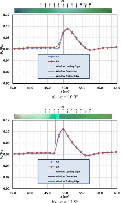
The final set of preliminary measurements was performed with the two shock generator configurations shown in Figure 10. The wall static pressure distributions on the upper
(AA) and lower (BB) positions are shown for the 10.0° and 13.5° shock generators in Figure 22(a) and (b), respectively. To estimate the shock impingement location, surface flow visualization was performed using an oil and florescent dye mixture. These results are shown at the top of the figures. For both cases, symmetry between the upper and lower pressure tap positions is observed to be quite good. As anticipated, the interaction region for both cases is located in the vicinity of the window centerline. The magnitude of the peak pressure and the axial extent of the interaction region is, as expected, greater for the stronger interaction case. For the 10.0° case, the oil flow
shows a light line indicating the upstream influence of the shock impingement, but no flow separation appears to be present. This line also corresponds with the initial rise in wall pressure. For
the 13.5° case, the oil flow shows a small pooling of oil
indicating flow separation. The upstream edge of the pooling also corresponds with the initial rise in wall pressure.
Pitot pressure profiles were taken at twelve axial stations through the interaction region at position BB for the α = 10.0°
and 13.5° cases. The location of the profiles are indicated in Figure 22 and the profiles at all 12 stations are shown in Figure 23. The first profile is located at x = 43.2 cm and the remaining profiles are equally spaced at 1.28 cm increments. The profiles plotted are the Pitot pressure normalized by the plenum total pressure. The wall static pressure normalized by the nozzle exit static pressure (Pw/Pnoz) is also plotted as a dotted
line. At the first station it is reasonable to assume that the wall static pressure is constant across the boundary-layer. Boundary-layer parameters were calculated for this station and are summarized in Table 2. One of the conclusions from Reference 8 is that when the ratio of upstream boundary-layer thickness to duct radius is greater than 0.1, a planar two-dimensional analysis cannot be used to predict flow separation because changes in the boundary-layer properties are larger for conical incident shock waves in an axisymmetric duct. For the present case, the ratio of boundary-layer thickness to duct radius is 0.154 indicating that the axisymmetric analysis must be used.
The incident shock plotted in the figures is based on inviscid theory using the cone angle and Mach number at the cone tip. This cone tip Mach number was interpolated from measurements made at the nozzle and test section exits. For the first four profiles, horizontal lines are drawn from where the incident shock crosses the data station to the Pitot profile. For both cases, these lines are in excellent agreement with the shock position indicted by the Pitot probe. Also indicated by vertical lines on the first four profiles is the normal shock total pressure
ratio associated with Mach number at the cone tip. This agrees well with the measured normalized Pitot pressure below the incident shock.
The reflected shock shown in the plots is based on the location inferred from the Pitot pressure profiles. As expected, the presence of the boundary layer moves the virtual origin of the reflected shock upstream of the incident shock impingement location.
a) α = 10.0°
b) α = 13.5°
Figure 22.—Wall pressure through interaction region. 0.00 0.02 0.04 0.06 0.08 0.10 0.12 35.0 40.0 45.0 50.0 55.0 60.0 65.0 pw /pt,0 x (cm) AA BB
Window Leading Edge Window Centerline Window Trailing Edge
1 2 3 4 5 CL6 7 8 9 10 11 12 0.00 0.02 0.04 0.06 0.08 0.10 0.12 35.0 40.0 45.0 50.0 55.0 60.0 65.0 pw /pt,0 x (cm) AA BB
Window Leading Edge Window Centerline Window Trailing Edge
a) α = 10.0°
b) α = 13.5°
Concluding Remarks
A new facility for investigating a Mach 2.5, 2-D shock-wave boundary-layer interaction has been presented along with preliminary measurements characterizing the flowfield. The data generated, once vetted by uncertainty estimates and redundant measurements, is intended to be used for CFD validation efforts. The preliminary results indicate that the facility is suitable for this purpose. From these preliminary data, refined flowfield measurement stations and surface dynamic pressure locations will be identified. Once the mean flow field has been characterized by conventional pressure measurements, constant-voltage hot-wire anemometry and PIV will be used to characterize the turbulence field throughout the interaction region.
References
1. Settles, G.S., and Dodson, L.J., 1994, “Supersonic and Hypersonic Shock/Boundary-Layer Interaction Database,” AIAA Journal, Vol. 32, No. 7, pp. 1377-1383. 2. Settles, G.S., and Dodson, L.J., 1991, “Hypersonic Shock/Boundary-Layer Interaction Database,” NASA CR 177577.
3. Aeschliman, D.P., and Oberkampf, W.L., 1998, “Experimental Methodology for Computational Fluid Dynamics Code Validation,” AIAA Journal, Vol. 36, No. 5, pp. 733-741.
4. Benek, A.J., Suchyta, C.R., and Babinsky, H., 2013, “The Effect of Wind Tunnel Size on Incident Shock Boundary Layer Interaction Experiments,” AIAA Paper 2013-0862, 51st AIAA Aerospace Sciences Meeting, Grapevine, TX. 5. Bruce, P.J. K., Burton, D.M. F., Titchener, N.A., and
Babinsky, H., 2011, “Corner Effect and Separation in Transonic Channel Flows,” J. Fluid Mechanics, Vol. 679, pp. 247-262.
6. Rose, W.C., 1973, “The Behavior of a Compressible Turbulent Boundary Layer in a Shock-Wave-Induced Adverse Pressure Gradient,” NASA TN D-7092.
7. Seebaugh, W.R., Paynter, G.C., and Childs, M.E., 1968, “Shock-Wave Reflection from a Turbulent Boundary Layer with Mass Bleed,” J. Aircraft, Vol. 5, No. 5, pp. 461-467.
8. Seebaugh, W.R., and Childs, M.E., 1970, “Conical Shock-Wave Turbulent Boundary-Layer Interaction Including Suction Effects,” J. Aircraft, Vol. 7, No. 4, pp. 334-340.
9. Bean, H.S. (ed), 1971, Fluid Meters: Their Theory and Application, 6th Ed., American Society of Mechanical Engineers, New York.
10. Davis, D.O., Friedlander, D.J., Saunders, J.D., Frate, F.C., and Foster, L., 2012, “Calibration of the NASA GRC 16 Mass Flow Plug,” FEDSM2012-72266, 2012 ASME Fluids Engineering Division Summer Meeting, Puerto Rico, USA.
11. Towne, C., “Wind-US User’s Guide, Version 2.0,” Glenn Research Center, NASA/TM—2009-215804, Oct. 2009. 12. Menter, F.R., “Two-Equation Eddy Viscosity Turbulence
Models for Engineering Applications,” AIAA Journal, Vol. 32, No. 8, 1994, pp. 1598-1605.
13. Blumenthal, P.Z., 1995, “A PC Program for Estimating Measurement Uncertainty for Aeronautics Test Instrumentation,” AIAA Paper 1995-3072, 31st AIAA Joint Propulsion Conference and Exhibit, San Diego, CA. 14. van Driest, E.R., 1951, “Turbulent Boundary Layer in
Compressible Fluids,” J. Aeronautical Sciences, Vol. 18, pp. 145-160.