Forecasting Inflation Using Dynamic Model Averaging

(1)

WP 34-09

Gary Koop

University of Strathclyde

and

The Rimini Centre for Economic Analysis, Italy

Dimitris Korobilis

University of Strathclyde

and

The Rimini Centre for Economic Analysis, Italy

FORECASTING INFLATION USING

DYNAMIC MODEL AVERAGING

Copyright belongs to the author. Small sections of the text, not exceeding three paragraphs, can be used provided proper acknowledgement is given.

The Rimini Centre for Economic Analysis (RCEA) was established in March 2007. RCEA is a private, non-profit organization dedicated to independent research in Applied and Theoretical Economics and related fields. RCEA organizes seminars and workshops, sponsors a general interest journal The Review of Economic Analysis, and organizes a biennial conference: Small Open Economies in the Globalized World (SOEGW). Scientific work contributed by the RCEA Scholars is published in the RCEA Working Papers series.

The views expressed in this paper are those of the authors. No responsibility for them should be attributed to the Rimini Centre for Economic Analysis.

(2)

Forecasting In‡ation Using Dynamic Model

Averaging

Gary Koop

University of Strathclyde

Dimitris Korobilis

University of Strathclyde

June 2009

Abstract

There is a large literature on forecasting in‡ation using the generalized Phillips curve (i.e. using forecasting models where in‡ation depends on past in‡ation, the unemployment rate and other predictors). The present paper extends this literature through the use of econometric methods which incorporate dynamic model averag-ing. These not only allow for coe¢ cients to change over time (i.e. the marginal e¤ect of a predictor for in‡ation can change), but also allows for the entire forecasting model to change over time (i.e. di¤erent sets of predictors can be relevant at di¤er-ent points in time). In an empirical exercise involving quarterly US in‡ation, we …nd that dynamic model averaging leads to substantial forecasting improvements over simple benchmark approaches (e.g. random walk or recursive OLS forecasts) and more sophisticated approaches such as those using time varying coe¢ cient models.

Keywords: Bayesian, State space model, Phillips curve

JEL Classi…cation: E31, E37, C11, C53

Both authors are Fellows at the Rimini Centre for Economic Analysis. Address for correspondence: Gary Koop, Department of Economics, University of Strathclyde, 130 Rottenrow, Glasgow G4 0GE, UK. Email: [email protected]

(3)

1 Introduction

Forecasting in‡ation is one of the more important, but di¢ cult, exercises in macroeco-nomics. Many di¤erent approaches have been suggested. Perhaps the most popular are those based on extensions of the Phillips curve. This literature is too voluminous to sur-vey here, but a few representative and in‡uential papers include Ang, Bekaert and Wei (2007), Atkeson and Ohanian (2001), Groen, Paap and Ravazzolo (2008) and Stock and Watson (1999). The details of these papers di¤er, but the general framework involves a dependent variable such as in‡ation (or the change in in‡ation) and explanatory vari-ables including lags of in‡ation, the unemployment rate and other predictors. Recursive, regression-based methods, have had some success. However, three issues arise when using such methods.

First, the coe¢ cients on the predictors can change over time. For instance, it is commonly thought that the slope of the Phillips curve has changed over time. If so, the coe¢ cients on the predictors that determine this slope will be changing. More broadly, there is a large literature in macroeconomics which documents structural breaks and other sorts of parameter change in many time series variables (see, among many others, Stock and Watson, 1996). Recursive methods are poorly designed to capture such parameter change. It is better to build models designed to capture it.

Second, the number of potential predictors can be large. For instance, Groen, Paap and Ravazzolo (2008) consider ten predictors. Researchers working with factor models such as Stock and Watson (1999) typically have many more than this. The existence of so many predictors can result in a huge number of models. For instance, if the set of models

is de…ned by whether each of m potential predictors is included or excluded, then the

researcher has2m _{models. This raises substantive statistical problems for model selection}

strategies. In light of this, many authors have turned to Bayesian methods, either to do Bayesian model averaging (BMA) or to automate the model selection process. Examples in macroeconomics and …nance include Avramov (2002), Cremers (2002) and Koop and Potter (2004). Furthermore, computational demands can become daunting when the

research is facing 2m _models.

Third, the model relevant for forecasting can potentially change over time. For in-stance, the set of predictors for in‡ation may have been di¤erent in the 1970s than now. Or some variables may predict well in recessions but not in expansions. This kind of issue further complicates an already di¢ cult econometric exercise. That is, if the researcher has

2m _{models and, at each point in time, a di¤erent forecasting model may apply, then the}

(4)

is2m . Even in relatively simple forecasting exercises, it can be computationally infeasible

to forecast by simply going through all of these2m combinations. For this reason, to our

knowledge, there is no literature on forecasting in‡ation with many predictors where the coe¢ cients on those predictors may change over time and where a di¤erent forecasting model might hold at each point in time. A purpose of this paper is to …ll this gap.

In this paper, we consider a strategy developed by Raftery, Karny, Andrysek and Ettler (2007) which they refer to as dynamic model averaging or DMA. Their approach can also be used for dynamic model selection or DMS where a single (potentially di¤erent) model can be used as the forecasting model at each point in time. DMA or DMS seem ideally suited for the problem of forecasting in‡ation since they allow for the forecasting model to change over time while, at the same time, allowing for coe¢ cients in each model to evolve over time. They involve only standard econometric methods for state space models such as the Kalman …lter but (via some empirically-sensible approximations) achieve vast gains in computational e¢ ciency so as to allow DMA and DMS to be done in real time despite the computational problem described in the preceding paragraph.

We use these methods in the context of a forecasting exercise with quarterly US data from 1959Q1 through 2008Q2. We use two measures of in‡ation and …fteen predictors and compare the forecasting performance of DMA and DMS to a wide variety of alterna-tive forecasting procedures. DMA and DMS indicate that the set of good predictors for in‡ation changes substantially over time. Due to this, we …nd DMA and DMS to forecast very well (in terms of forecasting metrics such as log predictive likelihoods, MSFEs and MAFEs), in most cases leading to large improvements in forecast performance relative to alternative approaches.

2 Forecasting In‡ation

2.1 Generalized Phillips curve models

Many forecasting models of in‡ation are based on the Phillips curve in which current in‡ation depends only on the unemployment rate and lags of in‡ation and unemployment. Authors such as Stock and Watson (1999) include additional predictors leading to the so-called generalized Phillips curve. We take as a starting point, on which all models used in this paper build, the following generalized Phillips curve:

yt= +x0t 1 +

p

X

j=1

(5)

where yt is in‡ation which we de…ne as ln _PPt

t 1 , with Pt being a price index, and xt a

vector of predictors. This equation is relevant for forecasting at timet given information

through timet 1. When forecastingh >1periods ahead, the direct method of forecasting

can be used andyt and "t are replaced byyt+h 1 and "t+h 1 in (1).

In this paper we use quarterly data. We provide results for in‡ation as measured by the GDP de‡ator and by the consumer price index (CPI). As predictors, authors such as Stock and Watson (1999) consider measures of real activity including the unemployment rate. Various other predictors (e.g. cost variables, the growth of the money supply, the slope of term structure, etc.) are suggested by economic theory. Finally, authors such as Ang, Bekaert and Wei (2007) have found surveys of experts on their in‡ation expectations to be useful predictors. These considerations suggest the following list of potential predictors which we use in this paper. Precise de…nitions and sources are given in the Data Appendix.

UNEMP: unemployment rate.

CONS: the percentage change in real personal consumption expenditures. INV: the percentage change in private residential …xed investment.

GDP: the percentage change in real GDP.

HSTARTS: the log of housing starts (total new privately owned housing units). EMPLOY: the percentage change in employment (All Employees: Total Private Industries, seasonally adjusted).

PMI: the change in the Institute of Supply Management (Manufacturing): Purchas-ing Manager’s Composite Index.

WAGE: the percentage change in average hourly earnings in manufacturing. TBILL: three month Treasury bill (secondary market) rate.

SPREAD: the spread between the 10 year and 3 month Treasury bill rates. DJIA: the percentage change in the Dow Jones Industrial Average.

MONEY: the percentage change in the money supply (M1).

(6)

COMPRICE: the change in the commodities price index (NAPM commodities price index).

VENDOR: the change in the NAPM vendor deliveries index.

This set of variables is a wide one re‡ecting the major theoretical explanations of in‡ation as well as variables which have found to be useful in forecasting in‡ation in other studies.

2.2 Time Varying Parameter Models

Research in empirical macroeconomics often uses time varying parameter (TVP) models which are estimated using state space methods such as the Kalman …lter. A standard

speci…cation can be written, fort = 1; ::; T, as

yt = zt t+"t (2a)

t = t 1 + t: (2b)

In our case, yt is in‡ation,zt = [1;xt 1; yt 1; : : : ; yt p] is an1 m vector of predictors for

in‡ation (including an intercept and lags of in‡ation), t = t 1; t 1; t 1; : : : ; t p is

anm 1vector of coe¢ cients (states),"t

ind

N(0; Ht)and t ind

N(0; Qt). The errors, "t

and t, are assumed to be mutually independent at all leads and lags. Examples of recent

papers which use such models (or extensions thereof) in macroeconomics include Cogley and Sargent (2005), Cogley, Morozov and Sargent (2005), Groen, Paap and Ravazzolo (2008), Koop, Leon-Gonzalez and Strachan (2009), Korobilis (2009) and Primiceri (2005). The model given by (2a) and (2b) is an attractive one that allows for empirical insights which are not available with traditional, constant coe¢ cient models (even when the latter are estimated recursively). However, when forecasting, they have the potential drawback that the same set of explanatory variables is assumed to be relevant at all points in time.

Furthermore, if the number of explanatory variables inzt is large, such models can often

over-…t in-sample and, thus, forecast poorly.

Popular extensions of (2a) and (2b) such as TVP-VARs also include the same set of explanatory variables at all times and su¤er from the same problems. Even innovative extensions such as that of Groen, Paap and Ravazollo (2008) involve only a partial treat-ment of predictor uncertainty. In an in‡ation forecasting exercise, they use a model which modi…es the measurement equation to be:

(7)

yt= m

X

j=1

sj jtzjt+"t;

where jt and zjt denote the jth elements of t and zt. The key addition to their model

is sj 2 f0;1g. Details of the exact model used for sj are provided in Groen et al (2008).

For present purposes, the important thing to note is that it allows for each predictor for

in‡ation to either be included (ifsj = 1) or excluded (ifsj = 0), but thatsj does not vary

over time. That is, this model either includes a predictor at all points in time or excludes it at all points in time. It does not allow for the set of predictors to vary over time. It is the treatment of this latter issue which is the key addition provided by DMA.

2.3 Dynamic Model Averaging

To de…ne what we do this paper, suppose that we have a set of K models which are

characterized by having di¤erent subsets of zt as predictors. Denoting these by z(k) for

k = 1; ::; K, our set of models can be written as:

yt = z (k) t (k) t +" (k) t (3) (k) t+1 = (k) t + (k) t ;

"_t(k) is N 0; H_t(k) and (_tk) is N 0; Q(_tk) . Let Lt 2 f1;2; ::; Kg denote which model

applies at each time period, t =

(1)0 t ; ::; (K)0 t 0 and yt _{= (}_y

1; ::; yt)0. The fact that we

are letting di¤erent models hold at each point in time and will do model averaging justi…es

the terminology “dynamic model averaging”. To be precise, when forecasting time t

variables using information through timet 1, DMA involves calculatingPr (Lt=kjyt 1)

for k = 1; ::; K and averaging forecasts across models using these probabilities. DMS

involves selecting the single model with the highest value for Pr (Lt=kjyt 1) and using

this to forecast. Details on the calculation of Pr (Lt=kjyt 1) will be provided below.

Speci…cations such as (3) are potentially of great interest in empirical macroeconomics since they allow for the set of predictors for in‡ation to change over time as well as allowing the marginal e¤ects of the predictors to change over time. The problems with such a framework are that many of the models can have a large number of parameters (and, hence, risk being over-parameterized) and the computational burden which arises when

K is large implies that estimation can take a long time (a potentially serious drawback

(8)

To understand the source and nature of these problems, consider how the researcher might complete the model given in (3). Some speci…cation for how predictors enter/leave the model in real time is required. A simple way of doing this would be through a

transition matrix,P, with elementspij = Pr (Lt=ijLt 1 =j) fori; j = 1; ::; K. Bayesian

inference in such a model is theoretically straightforward, but will be computationally

infeasible since P will typically be an enormous matrix. Consider the case where we have

m potential predictors and our models are de…ned according to whether each is included

or excluded. Then we have K = 2m _and _P _{is a} _K _K _{matrix. Unless} _m _{is very small,}

P will have so many parameters that inference will be very imprecise and computation

very slow.1 Thus, a full Bayesian approach to DMA can be quite di¢ cult. In this paper,

we use approximations suggested by Raftery, Karny, Andrysek and Ettler (2007) in an industrial application. These approximations have the huge advantage that standard state space methods (e.g. involving the Kalman …lter) can be used, allowing for fast real time forecasting.

The approximations used by Raftery et al (2007) involve two parameters, and ,

which they refer to asforgetting factors and …x to numbers slightly below one. To explain

the role of these forgetting factors, …rst consider the standard state space model in (2a)

and (2b). For given values of Ht and Qt, standard …ltering and smoothing results can

be used to carry out recursive estimation or forecasting. That is, Kalman …ltering begins with the result that

t 1jyt 1 N bt 1; t 1jt 1 (4)

where formulae for bt 1 and t 1jt 1 are standard (and are provided below for the case

considered in this paper). Note here only that these formulae depend onHtandQt. Then

Kalman …ltering proceeds using:

tjyt 1 N bt 1; tjt 1 ; (5)

where

tjt 1 = t 1jt 1+Qt:

Raftery et al (2007) note that things simplify substantially if this latter equation is re-placed by:

1_{See, for instance, Chen and Liu (2000) who discuss related models and how computation time up to} ttypically involves mixing overKtterms.

(9)

tjt 1 =

1

t 1jt 1 (6)

or, equivalently, Qt = 1 1 t 1jt 1 where 0 < 1. Such approaches have long

been used in the state space literature going back to Fagin (1964) and Jazwinsky (1970). Raftery et al (2007) provide a detailed justi…cation of this approximation and relate the resulting approach to statistical methods such as age-weighting and windowing and the reader is referred to their paper for details. The name “forgetting factor”is suggested by

the fact that this speci…cation implies that observationsj periods in the past have weight

j_{. An alternative way of interpreting} _{is to note that it implies an e¤ective window}

size of ₁1 . It is common to choose a value of near one, suggesting a gradual evolution

of coe¢ cients. Raftery et al (2007) set = 0:99. For quarterly macroeconomic data,

this suggests observations …ve years ago receive approximately 80% as much weight as last period’s observation. This is the sort of value consistent with fairly stable models

where coe¢ cient change is gradual. With = 0:95, observations …ve years ago receive

only about 35% as much weight as last period’s observations. This suggests substantial parameter instability where coe¢ cient change is quite rapid. This seems to exhaust the

range of reasonable values for and, accordingly, in our empirical work we consider

2(0:95;0:99). = 0:99will be our benchmark choice and most of our empirical results

will be reported for this (although we also include an analysis of the sensitivity to this choice).

An important point to note is that, with this simpli…cation, we no longer have to

estimate or simulate Qt. Instead, all that is required (in addition to the Kalman …lter) is

a method for estimating or simulating Ht (something which we will discuss below).

Forecasting in the one model case is then completed by the updating equation:

tjyt N bt; tjt ; (7) where b_t=bt 1+ tjt 1zt Ht+zt tjt 1zt0 1 yt ztbt 1 (8) and tjt= tjt 1 tjt 1zt Ht+zt tjt 1zt0 1 zt tjt 1: (9)

(10)

ytjyt 1 N ztbt 1; Ht+zt tjt 1zt0 : (10)

We stress that, conditional on Ht, these results are all analytical and, thus, no Markov

chain Monte Carlo (MCMC) algorithm is required. This greatly reduces the computa-tional burden.

The case with many models, (3), uses the previous approximation and an additional one. To explain this, we now switch to the notation for the multiple model case in (3)

and let t denote the vector of all the coe¢ cients. In the standard single model case,

Kalman …ltering is based on (4), (5) and (7). In the multi-model case, for modelk, these

three equations become:

t 1jLt 1 =k; yt 1 N b (k) t 1; (k) t 1jt 1 ; (11) tjLt=k; yt 1 N b (k) t 1; (k) tjt 1 (12) and tjLt =k; yt N b (k) t ; (k) tjt ; (13)

where b(_tk); _t(_jk_t) and (_t_jk_t)₁ are obtained via Kalman …ltering in the usual way using (8),

(9) and (6),except with (k) superscripts added to denote model k. To make clear the

notation in these equations, note that, conditional onLt =k, the prediction and updating

equations will only provide information on (tk)and not the full vector t. Hence, we have

only written (11), (12) and (13) in terms of the distributions which hold for (tk).

The previous results were all conditional onLt =k, and we need a method for

uncon-ditional prediction (i.e. not conuncon-ditional on a particular model). In theory, a nice way of

doing this would be through specifying a transition matrix, P, such as that given above

and using MCMC methods to obtain such unconditional results. However, for the rea-sons discussed previously, this will typically be computationally infeasible and empirically undesirable due to the resulting proliferation of parameters. In this paper, we follow the suggestion of Raftery et al (2007) involving a forgetting factor for the state equation for

the models, , comparable to the forgetting factor used with the state equation for

the parameters. The derivation of Kalman …ltering ideas begins with (4). The analogous result, when doing DMA, is

(11)

p t 1; Lt 1jyt 1 =

K

X

k=1

p (_tk)_1jLt 1 =k; yt 1 Pr Lt 1 =kjyt 1 ; (14)

wherep (_tk)₁_jLt 1 =k; yt 1 is given by (11). To simplify notation, let tjs;l = Pr (Lt=ljys)

and thus, the …nal term on the right hand side of (14) is t 1jt 1;k.

If we were to use the unrestricted matrix of transition probabilities inP with elements

pkl then the model prediction equation would be:

tjt 1;k = K

X

l=1

t 1jt 1;lpkl;

but Raftery et al (2007) replace this by:

tjt 1;k =

t 1jt 1;k

PK

l=1 t 1jt 1;l

; (15)

where0< 1is set to a …xed value slightly less than one and is interpreted in a similar

manner to . Raftery et al (2007) argue that this is an empirically sensible simpli…cation and, in particular, is a type of multiparameter power steady model used elsewhere in the literature. See also Smith and Miller (1986) who work with a similar model and argue approximations such as (15) are sensible and not too restrictive.

The huge advantage of using the forgetting factor in the model prediction equation

is that we do not require an MCMC algorithm to draw transitions between models nor a

simulation algorithm over model space.2 _{Instead, simple evaluations comparable to those}

of the updating equation in the Kalman …lter can be done. In particular, we have a model updating equation of:

tjt;k =

tjt 1;kpk(ytjyt 1)

PK

l=1 tjt 1;lpl(ytjyt 1)

; (16)

where pl(ytjyt 1) is the predictive density for model l (i.e. the Normal density in (10)

with (l) superscripts added) evaluated at yt.

Recursive forecasting can be done by averaging over predictive results for every model

using tjt 1;k. So, for instance, DMA point predictions are given by:

2_{Examples of simulation algorithms over model space include the Markov chain Monte Carlo model}

composition (MC3_{) algorithm of Madigan and York (1995) or the reversible jump MCMC algorithm of}

(12)

E ytjyt 1 = K X k=1 tjt 1;kz (k) t b (k) t 1:

DMS proceeds by selecting the single model with the highest value for tjt 1;k at each

point in time and simply using it for forecasting.

To understand further how the forgetting factor can be interpreted, note that this

speci…cation implies that the weight used in DMA which is attached to model k at time

t is: tjt 1;k / t 1jt 2;kpk yt 1jyt 2 = t 1 Y i=1 pk yt ijyt i 1 i :

Thus, modelk will receive more weight at timet if it has forecast well in the recent past

(where forecast performance is measured by the predictive density, pk(yt ijyt i 1)). The

interpretation of “recent past” is controlled by the forgetting factor, and we have the

same exponential decay at the rate i for observationsiperiods ago as we had associated

with . Thus, if = 0:99(our benchmark value and also the value used by Raftery et al,

2007), forecast performance …ve years ago receives 80% as much weight as forecast

per-formance last period (when using quarterly data). If = 0:95, then forecast performance

…ve years ago receives only about 35% as much weight. These considerations suggest that,

as with , we focus on the interval ₂(0:95;0:99).

Note also that, if = 1, then tjt 1;k is simply proportional to the marginal likelihood

using data through time t 1. This is what standard approaches to BMA would use. If

we further set = 1, then we obtain BMA using conventional linear forecasting models

with no time variation in coe¢ cients. In our empirical work, we include BMA in our set

of alternative forecasting procedures and implement this by setting = = 1.

We stress that, conditional on Ht, the estimation and forecasting strategy outlined

above only involves evaluating formulae such as those in the Kalman …lter. All the

recursions above are started by choosing a prior for 0j0;k and

(k)

0 for k= 1; ::; K.

The preceding discussion is all conditional on Ht. Raftery et al (2007) recommend

a simple plug in method where H_t(k) = H(k) _{and is replaced with a consistent estimate.}

When forecasting in‡ation, however, it is likely that the error variance is changing over

time. In theory, we could use a stochastic volatility or ARCH speci…cation for H_t(k).

(13)

simple plug-in approach which is a rolling version of the recursive method of Raftery et al (2007). To be precise, let e H_t(k)= 1 t t X j=t t +1 yt zt(k)b (k) t 1 2 z_t(k) _t(_jk_t) ₁z_t(k)0 :

Raftery et al (2007) uses this witht =t, but to allow for more substantial change in the

error variances (e.g. due to the Great Moderation of the business cycle), we set t = 20

and, thus, use a rolling estimator based on …ve years of data. Following Raftery et al

(2007), we can avoid the rare possibility thatHe_t(k) <0, by replacing H_t(k) byHb_t(k) where:

b H_t(k) = ( e H_t(k) if He_t(k) >0 b H_t(k)₁ otherwise :

3 Empirical Work

Our empirical work is divided into three sub-sections. The …rst two of these sub-sections present results using DMA and DMS, implemented in our preferred way. This involves

setting = 0:99, = 0:99, a noninformative prior over over the models (i.e. 0j0;k = _K1 for

k = 1; ::; K so that, initially, all models are equally likely) and a relatively di¤use prior on

the initial conditions of the states: (0k) N(0;100) fork = 1; ::; K. The …rst sub-section

presents evidence on which variables are good for predicting in‡ation. The second sub-section investigates forecast performance by comparing DMA forecasts to those produced by several alternative forecasting strategies. The third sub-section presents evidence on the sensitivity of our results to the choice of the forgetting factors. We present results

for short-term (h= 1), medium-term (h= 4) and long-term (h= 8) forecast horizons for

two measures of in‡ation: one based on the CPI, the other based on the GDP de‡ator. The list of potential predictors (which speci…es the transformation used on each variable) is given in sub-section 2.1 (see also the Data Appendix). All of our models include an

intercept two lags of the dependent variable.3

3.1 Which Variables are Good Predictors for In‡ation?

In theory, DMA has a large potential bene…t over other forecasting approaches in that it allows the forecasting model to change over time. Of course, in a particular empirical application, this bene…t may be small if the forecasting model does not change much over 3_{Preliminary experimentation with lag lengths up to four indicated two lags leads to the best forecast}

(14)

time. Accordingly, we begin by presenting evidence that, when forecasting in‡ation, the forecasting model is changing over time.

One striking feature of all of our empirical results is that, although we have 15 poten-tial predictors (and, thus, tens of thousands of models), most probability is attached to

very parsimonious models with only a few predictors. If we let Sizek be the number of

predictors in modelk (note thatSizek does not include the intercept plus two lags of the

dependent variable which are common to all models), then

E(Sizet) = K

X

k=1

tjt 1;kSizek

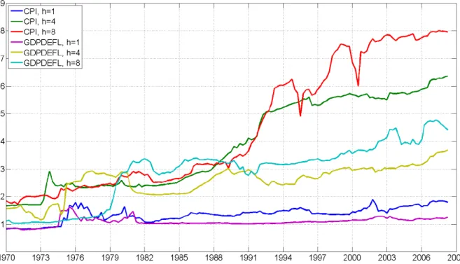
can be interpreted as the expected or average number of predictors used in DMA at time

t. Figure 1 plots this for our six empirical exercises (i.e. two de…nitions of in‡ation and

three forecast horizons).

For the short forecast horizon (h= 1), the shrinkage of DMA is particularly striking. It

consistently includes (in an expected value sense) a single predictor for both our de…nitions

of in‡ation. For GDP de‡ator in‡ation at horizons h = 4 and h = 8, slightly more

predictors are included (i.e. roughly 2 predictors are included in the early 1970s, but the number of predictors increases to 3 or 4 by the end of the sample). It is only for CPI based in‡ation at longer horizons that DMA chooses larger numbers of predictors. For

instance, for h = 8 the expected number of predictors gradually increases from about

two in 1970 to about eight by 2000. But even this least parsimonious case (which is still very parsimonious before 1990) excludes (in an expected value sense) half of the potential predictors.

Figure 1 shows clear evidence that DMA will shrink forecasts and provides some evidence that the way this shrinkage is done changes over time. But it does not tell us which predictors are important and how the predictors are changing over time. It is to these issues we now turn.

(15)

Figure 1: Expected Number of Predictors in Each Forecasting Exercise

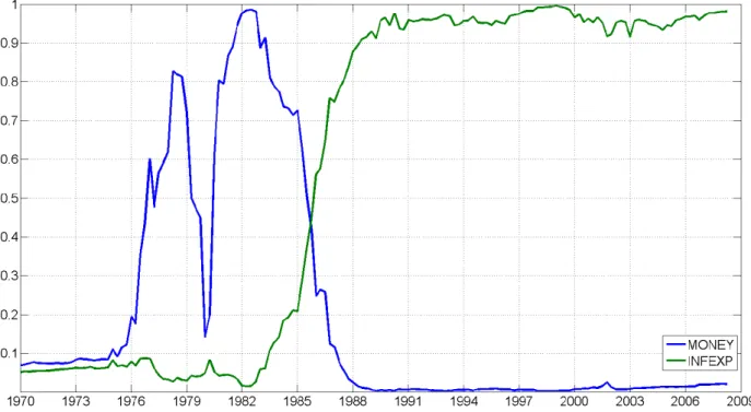
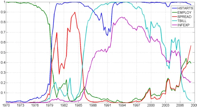
Figures 2 through 7 shed light on which predictors are important at each point in time for each of our six empirical exercises. These graphs contain posterior inclusion probabilities. That is, they are the probability that a predictor is useful for forecasting at

timet. Equivalently, they are the weight used by DMA attached to models which include

a predictor. To keep the …gures readable, we only present posterior inclusion probabilities for predictors which are important at least one point in time. To be precise, any predictor where the inclusion probability is never above 0.5 is excluded from the appropriate …gure. These …gures con…rm that DMS is almost always choosing parsimonious models and the weights in DMA heavily re‡ect parsimonious models. That is, with the partial

ex-ception of h = 8, it is rare for DMS to choose a model with more than two or three

predictors.

Another important result is that for both measures of in‡ation and for all forecast horizons, we are …nding strong evidence of model change. That is, the set of predictors in the forecasting model is changing over time.

Results for CPI in‡ation forh= 1 are particularly striking. Before 1975, no predictors

come through strongly. Between 1975 and 1985 money is the only predictor. After 1985 the measure of in‡ation expectations comes through strongly. With regards to the

in‡ation expectations variable, similar patterns are observed forh = 4and h= 8. Before

the mid- to late- 1980s there is little or no evidence that it is a useful predictor for in‡ation. But after this, it often is a useful predictor. To a lesser extent, the same pattern holds

(16)

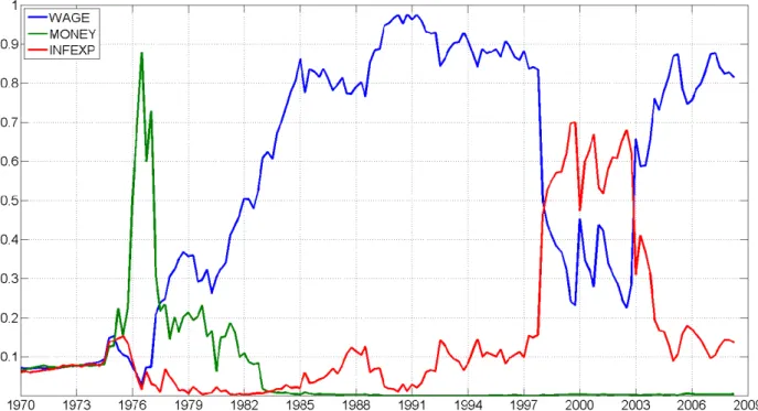
with GDP de‡ator in‡ation. For instance, with h = 1 very few predictors are included, with money being an important predictor near the beginning of the sample and in‡ation expectations being important near the end. However, for GDP de‡ator in‡ation with

h = 1, the predictor re‡ecting earnings (WAGE) comes through as being the strongest

predictor after 1980 (this variable was not found to be an important predictor for CPI in‡ation).

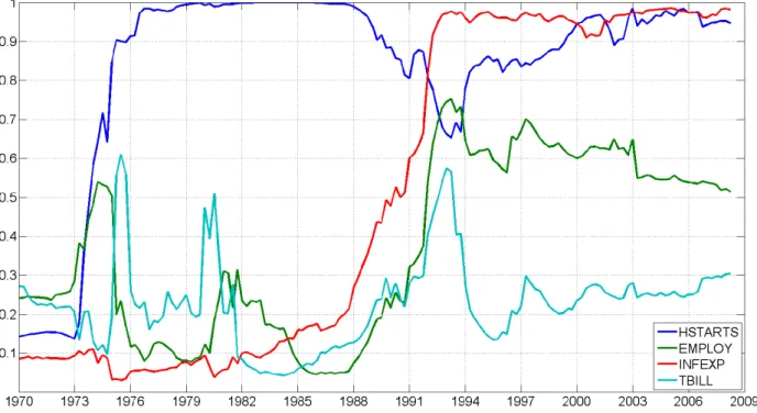
Housing starts is another variable which often has strong predictive power for both

measures of in‡ation. But, interestingly, only at medium or long horizons. For h = 1,

there is no evidence at all that housing starts have predictive power for in‡ation.

The interested reader can examine Figures 2 through 7 for any particular variable of interest. Most of our potential explanatory variables come through as being important at some time, for some forecast horizon for some measure of in‡ation. Only CONS, DJIA, COMPRICE and PMI never appear in Figures 2 through 7. But it is clearly the case that there is a large variation over time, over forecast horizons and over measures of in‡ation in what is a good predictor for in‡ation. We stress that the great bene…t of DMA and DMS is that they will pick up good predictors automatically as the forecasting model evolves over time.

(17)

Figure 3: Posterior Probability of Inclusion of Main Predictors (CPI in‡ation,h= 4)

(18)

Figure 5: Posterior Probability of Inclusion of Main Predictors (GDP de‡ator in‡ation,

h= 1)

(19)

h= 8) .

3.2 Forecast Performance: DMA versus Alternative Forecast

Procedures

There are many metrics for evaluating forecast performance and many alternative fore-casting methodologies that we could compare our DMA and DMS forecasts to. In this paper, we present two forecast comparison metrics involving point forecasts. These are mean squared forecast error (MSFE) and mean absolute forecast error (MAFE). We also present a forecast metric which involves the entire predictive distribution: the sum of log predictive likelihoods. Predictive likelihoods are motivated and described in many places such as Geweke and Amisano (2007). The predictive likelihood is the predictive density

for yt (given data through time t 1) evaluated at the actual outcome. The formula for

the one-step ahead predictive density in modellwas denoted bypl(ytjyt 1)above and can

be calculated as described in Section 2.3. We use the direct method of forecasting and,

hence, the log predictive density for the h-step ahead forecast is the obvious extension of

this. We use the sum of log predictive likelihoods for forecast evaluation, where the sum begins in 1970Q1. MSFEs and MAFEs are also calculated beginning in 1970Q1.

(20)

Forecasts using DMA with = = 0:99.

Forecasts using DMS with = = 0:99.

Forecasts using a single model containing all the predictors, but with time varying parameters (i.e. this is a special case of DMA or DMS where 100% of the prior weight is attached to the model with all the predictors, but all other modelling

choices are identical including = 0:99). This is labelled TVP in the tables.

Forecasts using DMA, but where the coe¢ cients do not vary over time in each model

(i.e. this is a special case of DMA where = 1).

Forecasts using BMA (i.e. this is a special case of DMA where = = 1).

Recursive OLS forecasts using an AR(2) model. Recursive OLS forecasts using all of the predictors. Random walk forecasts.

The …nal three methods are not Bayesian, so no predictive likelihoods are presented for these cases.

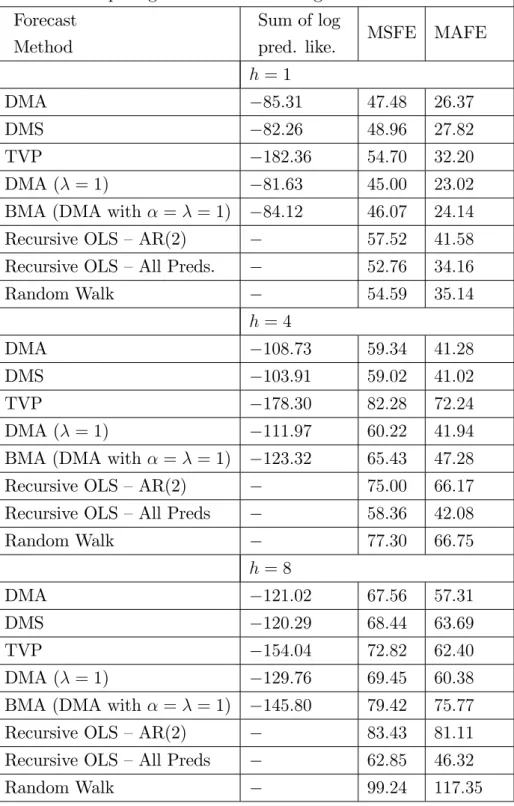
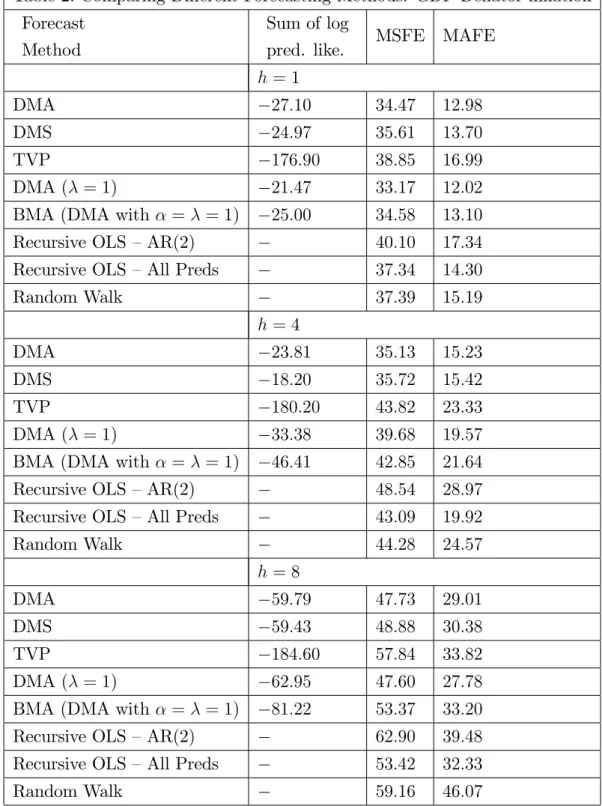
Tables 1 and 2 present results for our forecasting exercise for our two di¤erent measures of in‡ation. The big picture story is a clear and strong one: DMA and DMS forecast well. In most cases much better than other forecasting methods and in no case much worse than the best alternative method. We elaborate on these points below.

Consider …rst the log predictive likelihoods (the preferred method of Bayesian forecast comparison). These always indicate that DMA or DMS forecasts best. One message coming out of Tables 1 and 2 is that simply using a TVP model with all predictors leads to very poor forecasting performance. Of course, we are presenting results for only a single empirical exercise. But TVP models such as TVP-VARs are gaining increasing popularity in macroeconomics and the very poor forecast performance of TVP models found in Tables 1 and 2 should serve as a caution to users of such models (at least in forecasting exercises). Clearly, we are …nding that the shrinkage provided by DMA or DMS is of great value in forecasting.

DMA and DMS extend conventional forecasting approaches by allowing for model evolution and parameter evolution. A message provided by the predictive likelihoods is that most of the improvements in forecasting performance found by DMA or DMS are due to their treatment of model evolution rather than parameter evolution. That is, DMA with constant coe¢ cient models typically forecasts fairly well and occasionally even leads

(21)

to the best forecast performance (see the results in Tables 1 and 2 for h = 1). Recently, macroeconomists have been interested in building models involving parameter change of various sorts. Our results suggest that allowing for the model to change is at least as important. At short horizons, conventional BMA forecasts fairly well, but at longer horizons it tends to forecast poorly.

Predictive likelihoods also consistently indicates that DMS forecasts a bit better than DMA (although this result does not carry over to MAFEs and MSFEs where DMA tends to do better). DMS and DMA can be interpreted as doing shrinkage in di¤erent ways. DMS puts zero weight on all models other than the one best model, thus “shrinking” the contribution of all models except one towards zero. It could be that this additional shrinkage provides some additional forecast bene…ts over DMA.

If we turn our attention to results using MSFE and MAFE, we can see that the previous picture still holds (although DMA does somewhat better relative to DMS than we found using predictive likelihoods). In addition, we can say that naive forecasting methods such as using an AR(2) or random walk model are clearly inferior to DMA and DMS for both measures of in‡ation at all forecast horizons. However, with CPI in‡ation, recursive OLS

forecasting using all the predictors does well at the long horizon (h = 8). Forecasting

at such a long horizon is di¢ cult to do, so it is unclear how much weight to put on this result (and predictive likelihoods for this non-Bayesian method are not calculated). But it is worth noting that the good performance of recursive OLS in this case is not repeated for in‡ation measured using the GDP de‡ator nor at shorter horizons.

(22)

Table 1: Comparing Di¤erent Forecasting Methods: CPI in‡ation Forecast

Method

Sum of log

pred. like. MSFE MAFE

h = 1

DMA 85:31 47:48 26:37

DMS 82:26 48:96 27:82

TVP 182:36 54:70 32:20

DMA ( = 1) 81:63 45:00 23:02

BMA (DMA with = = 1) 84:12 46:07 24:14

Recursive OLS –AR(2) 57:52 41:58

Recursive OLS –All Preds. 52:76 34:16

Random Walk 54:59 35:14 h = 4 DMA 108:73 59:34 41:28 DMS 103:91 59:02 41:02 TVP 178:30 82:28 72:24 DMA ( = 1) 111:97 60:22 41:94

BMA (DMA with = = 1) 123:32 65:43 47:28

Recursive OLS –All Preds 58:36 42:08

BMA (DMA with = = 1) 145:80 79:42 75:77

(23)

Table 2: Comparing Di¤erent Forecasting Methods: GDP De‡ator in‡ation Forecast

Method

Sum of log

h = 1

DMA 27:10 34:47 12:98

DMS 24:97 35:61 13:70

TVP 176:90 38:85 16:99

DMA ( = 1) 21:47 33:17 12:02

BMA (DMA with = = 1) 25:00 34:58 13:10

BMA (DMA with = = 1) 46:41 42:85 21:64

BMA (DMA with = = 1) 81:22 53:37 33:20

Random Walk 59:16 46:07

3.3 Sensitivity Analysis

Our previous DMA and DMS results were for our benchmark case where = = 0:99.

As discussed previously, researchers in this …eld choose pre-selected values for and

(24)

It would be possible to choose and in a data-based fashion, but this is typically not done for computational reasons. For instance, the researcher could select a grid of values for these two forgetting factors and then do DMA at every possible combination of values

for and . Some metric (e.g. an information criteria or the sum of log predictive

likelihoods through timet 1) could be used to select the preferred combination of and

at each point in time. However, this would turn an already computationally demanding

exercise to one which wasg2 _{times as demanding (where} _g _{is the number of values in the}

grid). Accordingly, researchers such as Raftery et al (2007) simply go with = = 0:99

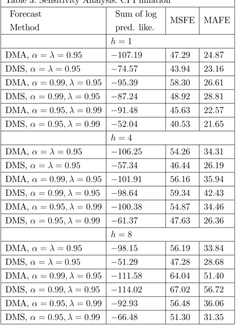
and argue that results will be robust to reasonable changes in these factors. In order to investigate such robustness claims, Tables 3 and 4 present results for our forecasting exercise using di¤erent combinations of the forgetting factors.

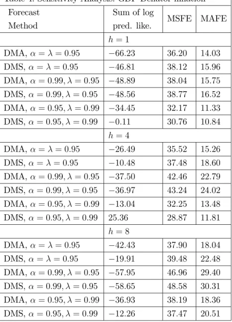
Overall, Tables 3 and 4 reveal a high degree of robustness to choice of and .

If anything, these tables emphasize the bene…ts of DMA in that measures of forecast performance are sometimes better than those in Tables 1 and 2 and rarely much worse.

One …nding of particular interest is that the combination = 0:95 and = 0:99

tends to forecast very well, for both of our measures of in‡ation. Note that the value

= 0:95allows for quite rapid change in forecasting model over time. This is consistent

with a story we have told before: that it appears that allowing for models to change over time is more important in improving forecast performance than allowing for parameters to change (at least in our data sets).

(25)

:

Table 3: Sensitivity Analysis: CPI in‡ation Forecast

Method

Sum of log

h= 1 DMA, = = 0:95 107:19 47:29 24:87 DMS, = = 0:95 74:57 43:94 23:16 DMA, = 0:99; = 0:95 95:39 58:30 26:61 DMS, = 0:99; = 0:95 87:24 48:92 28:81 DMA, = 0:95; = 0:99 91:48 45:63 22:57 DMS, = 0:95; = 0:99 52:04 40:53 21:65 h= 4 DMA, = = 0:95 106:25 54:26 34:31 DMS, = = 0:95 57:34 46:44 26:19 DMA, = 0:99; = 0:95 101:91 56:16 35:94 DMS, = 0:99; = 0:95 98:64 59:34 42:43 DMA, = 0:95; = 0:99 100:38 54:87 34:46 DMS, = 0:95; = 0:99 61:37 47:63 26:36 h= 8 DMA, = = 0:95 98:15 56:19 33:84 DMS, = = 0:95 51:29 47:28 28:68 DMA, = 0:99; = 0:95 111:58 64:04 51:40 DMS, = 0:99; = 0:95 114:02 67:02 56:72 DMA, = 0:95; = 0:99 92:93 56:48 36:06 DMS, = 0:95; = 0:99 66:48 51:30 31:35

(26)

:

Table 4: Sensitivity Analysis: GDP De‡ator in‡ation Forecast

Method

Sum of log

h= 1 DMA, = = 0:95 66:23 36:20 14:03 DMS, = = 0:95 46:81 38:12 15:96 DMA, = 0:99; = 0:95 48:89 38:04 15:75 DMS, = 0:99; = 0:95 48:56 38:77 16:52 DMA, = 0:95; = 0:99 34:45 32:17 11:33 DMS, = 0:95; = 0:99 0:11 30:76 10:84 h= 4 DMA, = = 0:95 26:49 35:52 15:26 DMS, = = 0:95 10:48 37:48 18:60 DMA, = 0:99; = 0:95 37:50 42:46 22:79 DMS, = 0:99; = 0:95 36:97 43:24 24:02 DMA, = 0:95; = 0:99 13:04 32:25 13:48 DMS, = 0:95; = 0:99 25:36 28:87 11:81 h= 8 DMA, = = 0:95 42:43 37:90 18:04 DMS, = = 0:95 19:91 39:48 22:48 DMA, = 0:99; = 0:95 57:95 46:96 29:40 DMS, = 0:99; = 0:95 58:65 48:58 30:31 DMA, = 0:95; = 0:99 36:93 38:19 18:36 DMS, = 0:95; = 0:99 12:26 37:47 20:51

4 Conclusions

This paper has investigated the use of DMA and DMS methods for forecasting US in-‡ation. These extend conventional approaches by allowing for the set of predictors for

in‡ation to change over time. When you have K models and a di¤erent one can

poten-tially hold at each of T points in time, then the resulting KT _{combinations can lead to}

serious computational and statistical problems (regardless of whether model averaging or model selection is done). As shown in this paper, DMA and DMS handle these problems in a simple, elegant and sensible manner.

In our empirical work, we present evidence indicating the bene…ts of DMA and DMS. In particular, it does seem that the best predictors for forecasting in‡ation are changing

(27)

considerably over time. By allowing for this change, DMA and DMS lead to substantial improvements in forecast performance.

(28)

References

Ang, A. Bekaert, G., Wei, M., 2007. Do macro variables, asset markets, or surveys forecast in‡ation better? Journal of Monetary Economics 54, 1163-1212.

Atkeson, A., Ohanian, L., 2001. Are Phillips curves useful for forecasting in‡ation? Federal Reserve Bank of Minneapolis Quarterly Review 25, 2-11.

Avramov, D., 2002. Stock return predictability and model uncertainty. Journal of Financial Economics 64, 423-458.

Chen, R., Liu. J., 2000. Mixture Kalman …lters. Journal of the Royal Statistical Society, Series B 62, 493-508.

Cogley, T., Sargent, T., 2005. Drifts and volatilities: Monetary policies and outcomes in the post WWII U.S.. Review of Economic Dynamics 8, 262-302.

Cogley, T., Morozov, S., Sargent, T., 2005. Bayesian fan charts for U.K. in‡ation: Forecasting and sources of uncertainty in an evolving monetary system. Journal of Eco-nomic Dynamics and Control 29, 1893-1925.

Cremers, K., 2002. Stock return predictability: A Bayesian model selection perspec-tive. Review of Financial Studies 15, 1223-1249.

Fagin, S., 1964. Recursive linear regression theory, optimal …lter theory, and error analyses of optimal systems. IEEE International Convention Record Part i, 216-240.

Geweke, J., Amisano, J., 2007. Hierarchical Markov normal mixture models with applications to …nancial asset returns.

Manuscript available at http://www.biz.uiowa.edu/faculty/jgeweke/papers/paperA/paper.pdf. Green, P., 1995. Reversible jump Markov chain Monte Carlo computation and Bayesian

model determination. Biometrika 82, 711-732.

Groen, J., Paap, R., Ravazzolo, F., 2008. Real-time in‡ation forecasting in a changing world. manuscript.

Jazwinsky, A., 1970. Stochastic Processes and Filtering Theory. New York: Academic Press.

Koop, G., Leon-Gonzalez, R., Strachan, R., 2009. On the evolution of the monetary policy transmission mechanism. Journal of Economic Dynamics and Control 33, 997-1017. Koop, G., Potter, S., 2004. Forecasting in dynamic factor models using Bayesian model averaging. The Econometrics Journal 7, 550-565.

Korobilis, D., 2009. Assessing the transmission of monetary policy shocks using dy-namic factor models. Discussion Paper 9-14, University of Strathclyde.

Madigan, D., York, J., 1995. Bayesian graphical models for discrete data. International Statistical Review 63, 215-232.

(29)

policy. Review of Economic Studies 72, 821-852.

Raftery, A., Karny, M., Andrysek, J. and Ettler, P., 2007. Online prediction un-der model uncertainty via dynamic model averaging: Application to a cold rolling mill. Technical report 525, Department of Statistics, University of Washington.

Smith, J. and Miller, J., 1986. A non-Gaussian state space model and application to prediction records. Journal of the Royal Statistical Society, Series B 48, 79-88.

Stock, J. and Watson, M., 1999. Forecasting in‡ation. Journal of Monetary Economics 44, 293-335.

Stock, J. and Watson, M.,1996. Evidence on structural instability in macroeconomic time series relations. Journal of Business and Economic Statistics 14, 11-30.

(30)

Data Appendix

The variables used in this study were taken from the sources in table below. All series were seasonally adjusted, where applicable, and run from 1959:Q1 to 2008:Q2. Some series in the database were observed on a monthly basis and quarterly values were computed by averaging the monthly values over the quarter. All variables are transformed to be

approximately stationary. In particular, if zi;t is the original untransformed series, the

transformation codes are (column Tcode below): 1 - no transformation (levels),xi;t =zi;t;

2 - …rst di¤erence, xi;t = zi;t zi;t 1 ; 4 - logarithm, xi;t = logzi;t; 5 - …rst di¤erence of

logarithm, xi;t = logzi;t logzi;t 1.

# Mnemonic Tcode Description Source

1 GDPDEFL 5 Gross Domestic Product: Implicit Price De‡ator FRED

2 CPI 5 Consumer Price Index For All Urban Consumers:

All Items

FRED

3 UNEMP 1 Civilian Unemployment Rate FRED

4 CONS 5 Real Personal Consumption Expenditures FRED

5 INV 5 Private Residential Fixed Investment FRED