Inflation dynamics and subjective expectations in the United States

WORKING PAPER NO. 222

INFLATION DYNAMICS AND

SUBJECTIVE EXPECTATIONS

IN THE UNITED STATES

BY KLAUS ADAM

AND MARIO PADULA

E U R O P E A N C E N T R A L B A N K

WORKING PAPER SERIES

WORKING PAPER NO. 222

INFLATION DYNAMICS AND

SUBJECTIVE EXPECTATIONS

IN THE UNITED STATES

1

BY KLAUS ADAM

2

AND MARIO PADULA

3

April 2003

E U R O P E A N C E N T R A L B A N K

WORKING PAPER SERIES

© European Central Bank, 2003

Address Kaiserstrasse 29

D-60311 Frankfurt am Main Germany

Postal address Postfach 16 03 19

D-60066 Frankfurt am Main Germany Telephone +49 69 1344 0 Internet http://www.ecb.int Fax +49 69 1344 6000 Telex 411 144 ecb d

All rights reserved.

Reproduction for educational and non-commercial purposes is permitted provided that the source is acknowledged. The views expressed in this paper do not necessarily reflect those of the European Central Bank.

Contents

Abstract

4

Non-technical summary

5

1

Introduction

7

2

Monopolistic price-setting with subjective expectations

9

3.

Data issues

10

4

Estimation results

12

5

Robustness of the results

15

5.1 Consistency of OLS estimates

15

5.2 Sub-sample stability

15

5.3 The role of lagged variables

16

6

Extension: the indexation model

17

7

Conclusions

18

8

Appendix

20

8.1 Subjective expectation and the NKPC

20

8.2 The data sources

21

References

21

9

Figures and tables

23

Abstract

We estimate a forward looking New Keynesian Phillips Curve (NKPC) for the U.S. using data from the Survey of Professional Forecasters as proxy for expected inflation. We obtain significant and plausible estimates for the structural parameters of the NKPC (the discount factor and the share of firms adjusting prices) independent from whether output or unit labor costs are used as a measure of marginal costs. Survey expectations suggest that the usual identification of expectations exploiting orthogonality of forecast errors with respect to output is severely distorted, which explains why the NKPC estimated with survey data performs much better than under the assumption of rational expectations. We also find that lagged inflation enters the price equation significantly, even when controlling for its ability to predict expectations. This suggests a role for lagged inflation beyond that of capturing non-rationalities in expectations. When estimating a Phillips curve where lagged inflation enters due to price indexation by non-reoptimizing firms, we find that rejection of the coe!cient restrictions depends on the measure of marginal costs used.

Keywords: Inflation, Phillips Curve, Subjective Expectations.

Non-technical summary

Recent papers have shown a revived interest in the ability of models with nominal price

rigidities to explain the dynamics of inflation rates. Among the different models under

scrutiny, forward looking New Keynesian models have become popular amongst researchers

and policy makers. These models generate a so-called New Keynesian Phillips Curve (NKPC)

that relates inflation rates to expected future inflation rates and the marginal costs of

production.

This paper estimates a forward looking NKPC for the United States. The main novelty of

the paper is that expected future inflation rates are measured using inflation survey data from

the Survey of Professional Forecasters.

Testing sticky price models with survey expectations is attractive since, to the extent that

survey data correctly capture agents’ expectations, it allows to disregard issues related to the

specification of agents’ expectations functions. One neither has to impose untested

orthogonality restrictions, as required when estimating under the assumption of rational

expectations, nor has to make restrictive assumptions about the precise form of non-rationality

present in agents’ forecasts. This allows to focus on the question whether the economic model

under consideration is correctly specified.

Previous tests of the NKPC have generated mixed results when performed under the

assumption that agents hold rational inflation expectations. More precisely, the empirical

success depended crucially on whether marginal production costs have been approximated by

the output gap or by unit labor costs.

Our main finding is that the NKPC performs equally well with both measures of

marginal costs, output and unit labor costs. Whatever measure is used, the estimate of the

quarterly discount factor is close to one and the point estimate of the degree of price stickiness

implies that firms reset their prices every four to five quarters on average.

These results suggests that potential non-rationalities in expectations, as they show up in

surveys, have biased rational expectations estimates that used the output gap to approximate

marginal costs. Quite surprisingly, the same non-rationalities do not seem to play a role when

using unit labor costs.

We show that the reason for this finding is that approximating the agents’ information set

using the unit labor cost variable rests on more solid grounds than approximating it using the

output variable. In particular, the survey data suggest that the hypothesis of rational

expectations implies a too high correlation between lagged output and future inflation

expectations. We show that this causes the coefficient estimate for the output gap to become

negative, contrary to what is implied by theory.

To check for the robustness of our findings, we include into the price equation lags of

various variables and test for their significance. While lagged measures of marginal costs

(unit labor costs and output) and lagged expectations remain insignificant, lagged inflation

enters significantly. Moreover, lagged inflation remains significant even when we account for

the fact that agents might use this variable to inform their inflation forecasts.

The significance of lagged inflation suggests that this variable plays a role in explaining

inflation dynamics that goes beyond explaining how actual inflation expectations might

deviate from rationality, contrary to what seems to be the predominant interpretation in the

recent literature.

To account for the role of lagged inflation we then estimate an inflation-indexation model

where lagged inflation enters because firms that do not optimally adjust prices are assumed to

index their prices using lagged inflation. We find that the data support the sign restrictions

implied by the model. Also, the more detailed parameter restrictions are not rejected when

output is used as the measure of marginal costs. However, these tend to be rejected with unit

labor costs.

Although the evidence is generally supportive of the NKPC, lagged inflation seems to be

a significant determinant of current inflation, even when taking care of potential

non-rationalities in inflation expectations. This fact cannot be reconciled with the standard New

Keynesian Phillips Curve and poses new questions for future research.

1

Introduction

This paper analyzes the ability of sticky price models to explain the dynamics of U.S. inflation when using survey data as proxies for inflation expectations.

Testing sticky price models with survey expectations is attractive since, to the extent that survey data correctly capture agents’ expectations, they allow to disregard issues related to the specification of agents’ expectations functions. One neither has to impose untested orthogonality restrictions, as required when estimating under the assumption of rational expectations, nor has to make restrictive assumptions about the precise form of non-rationality present in agents’ forecast functions. This allows to focus on the question whether the economic models under consideration are correctly specified.

Previous tests of sticky price models performed under the assumption that agents hold rational expectations have generated mixed results. Prominently, Fuhrer and Moore (1995) have reported that sticky price models do not generate su!cient stickiness for inflation when the output gap is used as a measure of real marginal costs.

Recent evidence, however, has shown that the empirical performance depends crucially on how one measures real marginal costs, the main determinant of inflation according to sticky price models. For instance, Galí and Gertler (1999) and Sbordone (2002) show that sticky price models perform well once marginal costs are approximated by average unit labor costs.1

It makes an important dierence whether sticky price models successfully explain inflation dy-namics as a function of output behavior or whether they relate inflation dydy-namics to the behavior of unit labor costs. Given that the ultimate objective is a model explaining the joint behavior of output and inflation, the latter case would require an additional empirically plausible theory linking the dynamics of unit labor costs to the behavior of output.

The present paper studies whether the currently popular New Keynesian Phillips Curve (NKPC), which can be derived from Calvo (1983) style sticky price models, is able to explain a relationship between inflation on the one hand and output or unit labor costs on the other hand. Thus, we let the data speak whether a theory linking output to costs is warranted, once expectations are approximated by data reported in the Survey of Professional Forecasters.

Our main finding is that the NKPC performs equally well with both measures of marginal costs, output and unit labor costs. Whatever measure is used, the estimate of the quarterly discount factor is close to one and the point estimate of the degree of price stickiness implies that firms reset their prices every four to five quarters on average.

These results suggests that potential non-rationalities in expectations, as they show up in surveys, have biased previous estimates using output as a measure for marginal costs. Quite surprisingly, the same non-rationalities do not seem to play a role when using unit labor costs. Here our estimates

1_{A dierent view about the ability of unit labor costs to explain U.S. inflation dynamics has recently been expressed}

confirm the results obtained by Galí and Gertler (1999) and Sbordone (2002) who assumed rational expectations.

We show that the reason for this finding is that approximating the agents’ information set using the unit labor cost variable rests on more solid grounds than approximating it using the output variable. In particular, the survey data suggests that the hypothesis of rational expectations implies a too high correlation between lagged output and future inflation expectations. We show that this causes the coe!cient estimate for output to become negative, contrary to what is implied by theory. These results suggest that once one takes account of potentially non-rational expectations via survey expectations, sticky price models are able to establish a close link between output dynamics and the behavior of inflation.

To check for the robustness of this finding, we include into the price equation lags of various variables and test for their significance. While lagged measures of marginal costs (unit labor costs and output) and lagged expectations remain insignificant, lagged inflation enters significantly. Moreover, lagged inflation remains significant even when we account for the fact that agents might use this variable to inform their inflation forecasts.

The significance of lagged inflation suggests that this variable plays a role in explaining infla-tion dynamics that goes beyond explaining how actual inflainfla-tion expectainfla-tions might deviate from rationality, contrary to what seems to be the predominant interpretation in the recent literature.

To account for the role of lagged inflation we estimated the inflation-indexation model of Chris-tiano, Eichenbaum, and Evans (2001) where lagged inflation enters because firms are assumed to index their prices using lagged inflation rates in periods where they do not adjust prices optimally. We find that the data support the sign restrictions implied by the model. The more detailed pa-rameter restrictions implied by this model are not rejected when output is used as the measure of marginal costs but tend to be rejected for the case of unit labor costs. Somewhat surprisingly, the share of reoptimizing firms is still estimated to be around one quarter for most specifications.2

Obviously, we are not the first to estimate sticky price models using survey expectations. Roberts (1995, 1997) estimated sticky price models using the Livingston and Michigan surveys and showed that sticky price models can account for inflation dynamics at a semi-annual or annual frequency. Since data in the Survey of Professional Forecasters is collected on a quarterly basis we can construct a quarterly model. Our estimates thereby remain more easily comparable to recent estimates based on quarterly data.

The paper is structured as follows. In section 2 we present conditions under which the first order conditions characterizing firms’ optimal pricing decision give rise to a New Keynesian Phillips Curve when expectations are potentially non-rational. Section 3 presents the data and assesses the rationality of survey expectations. The estimation results for the benchmark NKPC are presented in section 4 and their robustness is analyzed in section 5. Section 6 then presents the results for the inflation indexation model and a conclusion briefly summarizes.

2_{This suggests a prices are less but inflation is more sticky than implied by the standard NKPC without lagged}

2

Monopolistic Price-Setting with Subjective Expectations

This section derives the New Keynesian Phillips Curve for the case where expectations are subjective and potentially non-rational. The resulting Phillips curve will be similar to widely used specifications of Galí and Gertler (1999) and Roberts (1995). For illustrative purposes we use Calvo’s (1983) time-dependent pricing model to derive our results but similar reduced-form Phillips curve equations can be obtained using the quadratic adjustment cost model of Rotemberg (1982).

Firms in monopolistic competition must precommit to prices that can be reset with probability

15(0,1)each period. Firms’ forecasts are produced by professional forecasters. Each forecaster

i5{1, . . . I}thereby advises a fixed share 1_I of firms. The (subjective) forecast delivered by forecaster

iwill be denoted byF_ti[·].

LetPtdenote the aggregate price level at period t andP_ti the price chosen by a firm that can reset prices in periodtand is advised by forecasteri. Then the new price level can be expressed as

Pt= (1)1_I I X i=1 P,i t +Pt1 (1)

The new price level is a convex combination between the old price level and the average price selected by firms that adjust their price. Firms that reset prices maximize expected discounted profits, which are given by

max P,i t Fi t 5 7 4 X j=0 ()j à P,i t Pt+j !% (P,i t MCt+j) 6 8 ₍₂₎

where1is the discount factor, %>1is the elasticity of the demand function, andMC are the nominal marginal costs of production. Linearizing the first order conditions of this problem around a zero inflation steady state delivers

p,i t = (1)Fti 5 7 4 X j=0 ()jmct+j 6 8 ₍₃₎

where lower case variables denote percentage deviations from steady state. Under the assumption of rational expectations equations (1) and (3) can be used to derive the familiar New Keynesian Phillips Curve

_{t=Et[t+1] +} (1)(1)

rmct (4)

where current inflation is a function of (rational) inflation expectations and real marginal costsrmc_t. Deriving an equation similar to equation (4) when expectations are subjective is not entirely obvious. Profit-maximizing prices depend on nominal costs and therefore on forecasted inflation. Inflation is determined by other agents’ pricing decisions and their marginal cost forecasts. As a result, optimal price setting behavior would require forecasting the marginal cost forecasts of others,

see Woodford (2001) for a recent treatment. Obviously, expectations survey data do not report agents’ subjective forecasts of other agents’ forecasts. Therefore, we want to delineate conditions under which subjective inflation forecasts summarize all beliefs about other agents’ marginal cost expectations.

Suppose the following condition holds:

Condition 1

Fi

t£Fth+1[mct+s]Fth[mct+s]¤= 0 ;i, h, s >0 (5)

Condition 1 requires that agents do not expect that current forecasts of future variables will be revised in a particular direction in the next period, i.e. they do not expect predictable movements of their own or other agents’ expectations. This is the case whenever expectations fulfill the ’law of iterated expectations’.

Importantly, condition 1 does not rule out non-rationalities in expectations. Suppose, for ex-ample, that marginal costs are expected to follow an AR(1) process where multi-step forecasts are obtained by simply iterating the AR(1) equation. Condition 1 is then satisfied but expectations will be non-rational if actual inflation follows some other stochastic process.

Appendix 8.1 shows that whenever condition 1 holds, the subjective inflation forecast of the aggregate inflation rate is a su!cient statistic summarizing all forecasts of other agents’ forecasts. One then obtains a Phillips curve of the form:

t=Ft[t+1] + (1)(1 )rmct (6)

The only dierence to the Phillips curve in equation (4) is that rational expectations are now substituted by the average of the forecasters’ subjective expectations, which is defined as

Ft[·] = 1_I I X i Fi t[·] (7)

3

Data Issues

This section describes the data we use to estimate equation (6). A detailed description of the data sources and variable definitions is given in appendix 8.2.

We use quarterly U.S. data from 1968:4-2000:1 where the starting date is determined by the availability of inflation survey data. Inflation is calculated using the implicit GDP deflator.3 We use aggregate data instead of data for the non-farm private business sector, which is the usual activity measure used in the literature, because inflation forecasts are available only for aggregate deflators. Since non-farm private business accounts for approximately 85% of aggregate GDP our results can be expected to be comparable to the remaining literature. In any case, the broader activity measure should only strengthen the importance of our findings.

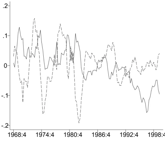
We use two measures for the real marginal costs in equation (6). Firstly, we use the unit labor costs, defined as the dierence between log compensation to employees and log nominal GDP in deviation from the sample average. This is the measure used by Galí and Gertler (1999) or Sbordone (2002).4 _{Secondly, we consider the output gap, obtained by detrending output with an HP-filter}

with smoothing parameter 1600.5 The output gap has been used by Fuhrer and Moore (1995), for example.

Figure 2 graphs the unit labor costs and the output gap. The figure shows that there is a negative contemporaneous correlation between the labor share and output, as was the case for the data used by Galí and Gertler (1999).

Inflation expectations are approximated with data from the Survey of Professional Forecasters. The survey collects data from around 80 professional forecasters on a quarterly basis from 1968 onwards. A description of the survey can be found in Croushore (1993). Given that we estimate a quarterly model, we use the mean of the one-quarter ahead inflation forecast for the implicit GDP deflator as the measure for expected inflation in equation (6).

Figure 1 plots actual and expected quarterly inflation rates and shows that actual and expected inflation rates move closely together over the sample period.6

To assess whether inflation forecasts are biased or ine!cient we perform a standard test. This test requires to regress actual inflation rates on a constant and on expected inflation rates and to check if the constant is equal to zero and the coe!cient in front of the expectations term equal to one. For our survey data this delivers:7

_t= 0.000

(0.001)+ 1(0..017100)Ft1[t] (8)

Since the coe!cient restrictions are not rejected, survey expectations seem to be consistent with rational expectations.

A closer look at figure 1, however, suggests that expected inflation is lagging actual inflation slightly. Indeed, it is not di!cult to find evidence that the survey expectations are ine!cient. In particular, the constant appearing in equation (8) is not equal to zero in various sub-periods. This is shown in table 1, which presents results from regressing forecast errors on a constant and dummy variables for the 1970’s and 1980’s, where the latter intend to capture dierent policy regimes.

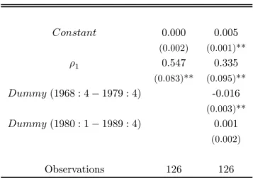
The estimates in table 1 show that inflation expectations have been significantly below actual inflation rates during the 1970’s and considerably above the actual rates during the 1980’s. This seems hardly surprising given that inflation rates were generally rising during the 1970’s but falling during the 1980’s and indicates that forecasts are far from being e!cient (see also Croushore (1996)). Table 2 presents further evidence on the time series structure of forecast errors. Column two of the table shows that forecast errors display significant positive autocorrelation. Correlation decreases only moderately when accounting for dierent policy regimes via time dummies in the third column.

4_{These authors use data for the non-farm private business sector only.} 5_{We also used quadratic detrending, which led to very similar results.}

6_{At each date the figure shows actual quarterly inflation and the forecast made for this rate in the previous quarter.} 7_{The values in parentheses are asymptotic Newey-West 4 lags standard errors.}

To the extent that survey expectations correctly capture inflation expectations the previous evidence shows that these expectations are ine!cient and, thus, can be biased during sub-periods. This suggests that forecast errors will generally not be orthogonal to information available to agents at the time of the forecast. This is important because instrumental variable techniques, which are commonly employed to estimate the NKPC under rational expectations, assume orthogonality of forecast errors with respect to lagged information.

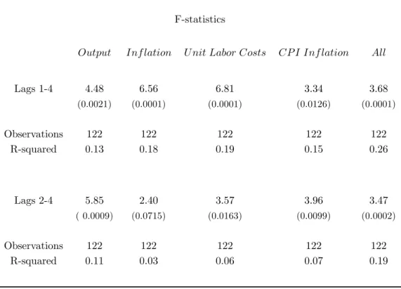
To check whether commonly used instruments are correlated with the forecast errors implied by the survey data, we regressed these errors on a constant and lags of output, inflation, unit labor costs, commodity price inflation, and all variables together. The upper panel of table 3 reports F-statistics testing the null hypothesis that the coe!cients on lags 1 to 4 of these regressors are jointly equal to zero. The hypothesis is strongly rejected in all cases. In the lower panel of table 3 we report the same test when regressing on lags 2 to 4 only, to check whether results are sensitive to the assumption that agents know the first lag of the considered variables. Results remain unchanged. To the extent that survey data correctly capture agents’ inflation expectations, these results cast doubts on the validity of Phillips curve estimates that have been derived under the assumption of rational expectations.

4

Estimation Results

This section presents the results from estimating equation (6) with the data set described in the previous section.

If theory was correct and all variables were measured without error, then equation (6) would perfectly fit the data. Obviously, this is highly implausible for a number of reasons. The time dependent pricing setting rules underlying equation (6) are at best an approximation to firms actual price setting behavior. Moreover, the variables entering equation (6) are not precisely measured by our data; this might hold for the GDP Deflator as well as for the two measures of real marginal cost. We proceed by assuming that deviations from equation (6) are due to measurement error. Con-sequently, we estimate

_t=F_t[_t+1] +rmc_t+%_t (9) where%t captures measurement errors and where

=(1)(1)

Measurement errors might aect the left-hand and right-hand side of equation (9). Errors af-fecting the left-hand side are of little concern since OLS estimators can deal with it. Measurement errors on the right-hand side, however, would require the use of instrumental variable (IV) estima-tors. Right-hand side errors could arise because we replaced the mean expected inflation by the sample average across forecasters or because of our approximate real marginal cost measures. Since

the consistency of OLS estimates cannot be rejected for our sample, as shown in section 5, we will report OLS estimates of equation (9) below.8

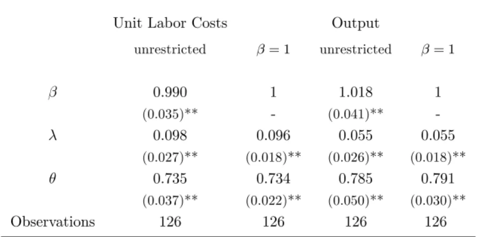
Table 4 shows the estimates of equation (9) when using the unit labor costs (column 2) and the output gap (column 4), respectively, as a measure for marginal costs.9 _{Independent from the}

specification of marginal costs, all coe!cients have the correct sign and are significant at the one percent level. In particular, the discount rate is close to one, as theory would predict, and the estimate ofis positive.

The value for the degree of price stickiness implied by the point estimates forandis also reported in the table. Independent from the marginal cost measure, the estimates suggests that about one forth of firms adjust prices every quarter, which causes prices to be reset once a year on average. This seems largely consistent with survey data on price stickiness, see Blinder et al. (1998). For completeness, columns three and five of table 4 report the results from restricting the discount factor to be equal to one, as commonly done in the empirical literature. This does not cause a sizeable change of the implied stickiness parameter.

The results for the case that real marginal costs are approximated by unit labor costs are in line with estimates obtained by Galí and Gertler (1999) who assumed inflation expectations to be rational.10 _{This is surprising since, as shown in table 3, the forecast errors implied by survey}

expectations are not orthogonal to lagged unit labor costs, which is an identification assumption made by these authors. This suggests that the distortion caused by such an identification assumption is not strong enough to seriously aect the parameter estimates. We will come back to this point below.

Even more surprising are the results reported for the output gap in table 4. It has been rather di!cult to obtain parameter estimates with the correct sign and of a plausible magnitude when using output as a measure for marginal costs. Fuhrer and Moore (1995) and Galí and Gertler (1999), for example, find a negative and insignificant estimate ofwhen real marginal costs are approximated by detrended output. Table 4, however, shows that with the help of survey expectations one can establish a plausible link between output and inflation dynamics via the NKPC. This suggests that the assumption of rational expectations is not innocuous in this case.

Why do non-rationalities seem to matter when using output but not when using labor costs as a measure for marginal costs? A detailed answer is given below.

For the case of unit labor costs, the correlation between next period’s actual inflation and marginal costs is of about the same size as the correlation between the subjective expectation of

8_{We also prefer OLS estimates to IV estimates because they avoid the problem of instrument choice to which IV}

estimates may be sensitive.

9_{Since Bartlett tests reject the null hypothesis that the residuals follow a white noise we use the Newey-West}

correction with four lags to compute the standard errors for the regression.

1 0_{Our point estimate for the degree of price stickiness is somewhat lower and the point estimate of the discount}

next period’s inflation and marginal costs. This suggests that inflation expectations incorporate large part of the information contained in current unit labor costs.11

The situation is quite dierent for the case of the output gap. There, the correlation between next period’s actual inflation and current output is much higher than the correlation between expected inflation and output. Thus, identifying restrictions that impose orthogonality of forecast errors with respect to current output impute too much information to expectations.

To see how a change in these correlations might induce a change in the sign of the estimated

-coe!cient consider the following expression for the regression coe!cient

= 1

A

¡

corr(_t, rmc_t)corr(F_t[_t+1], rmc_t)·B¢ (10)

where A is the determinant of a positive definite matrix and therefore always positive and B =

corr(Ft[t+1],t)is approximately equal to 0.8 and independent from whether subjective

expec-tations or actual future inflation rates are used as a proxy for expected inflation.12 Given this, the sign ofdepends mainly on the dierence betweencorr(_t, rmc_t)andcorr(F_t[_t+1], rmc_t).

Actual inflation is more strongly correlated with lagged output than with contemporaneous output. This is shown in figure 4, which depicts the correlations together with the 95% confidence intervals.13 Thus, the estimated coe!cient is negative (or insignificant) when output is used as a measure for real marginal costs and when actual inflation is the measure for expected inflation.14

When substituting actual inflation by subjective expectations the coe!cient turns positive again because the correlation between subjective inflation expectations and the output gap is much lower than the same correlation for actual inflation. This explains the changed sign for thecoe!cient.

When unit labor costs are used then the dierence in the correlation coe!cients is positive and almost independent from the measure of expected inflation (actual inflation or subjective forecasts). While corr(F_t[t+1], rmct) is smaller than corr(t, rmct) when expectations are subjective, as

one would expect, the same holds when expectations are rational. Figure 3 depicts the dynamic correlation between actual inflation and unit labor costs together with the 95% confidence intervals.15

The figure shows that both variables are contemporaneously correlated. Consequently, the coe!cient estimate remains positive when assuming rational expectations.

The previous results show that the NKPC can link inflation dynamics to both output and unit labor cost dynamics once survey data are used to proxy for inflation expectations. At the same time, survey data suggest that the identification of expectations assuming orthogonality with respect to

1 1_{The fact thatcorr(}

t+1, mct)Ecorr(Ft[t+1], mct)implies that in a regression of the forecast error(t+13

Ft[t+1])on a constant and marginal costsmc_tthe coe!cient in front ofmc_tis (approximately) equal to zero. Thus,

mctcannot explain the forecast errors. Obviously, this does not imply that forecasts contain the information in lagged values ofmc_t. Table 3 shows that this is not the case.

1 2_{corr(·,·)denotes the correlation coe!cient between two variables.}

1 3_{Confidence intervals have been computed using bootstrapped standard errors.}

1 4_{Taking actual inflation is similar to assuming that expectations are rational. It is identical when shocks are absent,}

i.e. in a perfect foresight equilibrium.

output is responsible for the unsatisfactory performance of the NKPC when using output as a measure for marginal costs.

5

Robustness of the Results

5.1

Consistency of OLS Estimates

Since measurement error may be present on the right-hand side of equation (9) we tested for the consistency of our OLS estimates. This can be done using the Hausman test which compares instrumental variable estimates with OLS estimates. The null hypothesis under scrutiny is that OLS generate consistent estimates of the parameters in equation (9).

We computed the Hausman test for both measures of real marginal costs. Since the qualitative results are identical we report only those obtained for unit labor costs.

The set of instruments used includes two lags of expected inflation and four lags of marginal costs.16 The instruments pass the Hansen-Sargan test with a statistic equal to 8.7630 which cor-responds to a p-value of 0.1189. F-tests strongly reject the hypothesis that the coe!cients in the regressions of expected inflation and marginal costs on the instruments are jointly equal to zero.17 TheR2of these regressions are 0.9301 and 0.8694 for expected inflation and marginal costs, respec-tively. This shows that the chosen instruments do not violate overidentifying restrictions and are correlated with the variables in the regression.

Estimating equation (9) with the chosen instruments and computing the Hausman statistic implies a p-value of 0.5378 for the null hypothesis that OLS estimates are consistent. This justifies the use of OLS estimates in the previous section.

5.2

Sub-Sample Stability

In this section we analyze the stability of the Phillips curve relationship by considering the estimates obtained from dierent sub-samples.

We split the sample into 3 approximately decade-long sub-periods: 1968:4-1979:4, 1980:1-1989:4, and 1990:1-2000:1. Splitting the data set in this way generates sub-samples with rather dierent inflation experiences. While inflation has been volatile and rising in the 1970’s, inflation dropped during the 1980’s and has been low and stable during the 1990’s, see figure 1.

To the extent that these dierences have been caused by dierences in the conduct of monetary policy, a test for parameter stability in the three sub-samples may be considered to be a test for the policy invariance of the price-setting assumption underlying the Calvo (1983) formulation of the NKPC.

1 6_{The use of lagged variables as instruments is legitimate if the measurement error has no structure (classical}

measurement error).

Table 5 reports the coe!cient estimates for the three sub-samples. Reassuringly, all coe!cients have the correct sign independent from the sample period and the measure of marginal costs used. However, real marginal cost do not always enter significantly in the 1980’s and do never so in the 1990’s. This lack of statistical insignificance may be partly due output and inflation not showing very much sample variation, at least during the last sub-sample period.

The Chow test rejects the hypothesis of sub-sample stability across the three periods indepen-dently from the measure of marginal cost used.18 For the specification using output one cannot reject that all sub-sample estimates of are equal to the estimate obtained for the whole sample. An analogous test for unit labor cost, however, rejects parameter constancy.

The estimates in table 5 also suggest that the discount factor has been higher during the 1970’s than during the 1980’s and 1990’s.19 Giving an economic interpretation to this finding seems di!cult in the light of the underlying theory.

Comparing the estimates for degree of price stickinessin table 5 suggests that price rigidity has been higher during the 1990’s than during the 1970’s. Thus, the underlying pricing rules seem not to be invariant to the inflation process, as one might expect. The higher and more variable inflation experience during the 1970’s might have caused firms to reset their prices more often than this was the case during the 1990’s where inflation was low and stable.

Overall, the picture emerging from the sub-samples is not too disappointing. Despite some impor-tant dierence across the dierent time periods, all estimates still have the correct sign. Moreover, there is no evidence that the performance of the Phillips curve depends on the measure of marginal costs used, which is the main finding obtained for the whole sample period.

5.3

The Role of Lagged Variables

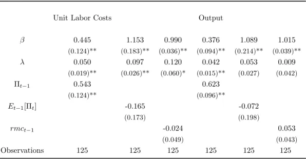
We now assess to what extent the data attribute a role to lagged variables in explaining inflation dynamics. This is done by adding lagged values of inflation, expected inflation, and marginal costs to equation (9). We consider this ad-hoc variation as a robustness check to see whether the data favor the Phillips curve of equation (9) or rather some alternative specification.

Table 6 reports the estimation results. Except for lagged inflation, which enters significantly in both specifications, all other lagged variables remain insignificant at the 5% level. When adding either lagged expectations or lagged marginal costs, the parameter estimates remain surprisingly close to the benchmark estimates reported in table 4. In particular, the discount factor remains close to one and the coe!cients on marginal costs still have the correct sign. Also the sum of the coe!cients on marginal costs remains close to their benchmark values.

The case with lagged inflation diers notably. Typically, the role for lagged inflation in the pricing equation is attributed to the presence of agents whose forecasts are not perfectly rational, see Galí

1 8_{The F-Statistics of the test are 23.17 and 19.66 for unit labor costs and output gaps, respectively.}

1 9_{A similar result appears in table 4 of Gali and Gertler (1999) for the case where the GDP-Deflator is used to}

and Gertler (1999) or Roberts (1997). In the current setting this interpretation is inappropriate because we have accounted for potential non-rationalities in expectations through the use of survey data. Nevertheless, it is conceivable that lagged inflation enters significantly due to non-rationalities only: since the survey expectations are likely to depend on lagged inflation rates, expected inflation and lagged inflation tend to be collinear and the coe!cient on lagged inflation might capture variation in lagged inflation that should be attributed to expected inflation.20

To assess whether lagged inflation has explanatory power for inflation dynamics beyond its abil-ity to predict expected inflation we perform the following exercise: we regress lagged inflation on expected inflation and include the regression residuals into the standard specification (9) as an additional regressor.

Intuitively, the regression residuals represent that part of the variation of lagged inflation which is orthogonal to expected inflation and, thus, does not explain variations in expectations. It should be clear that by including only these residuals into the pricing equation when testing for the significance of lagged inflation, we bias results in favor of rejecting a role for lagged inflation.

Nevertheless, we find that the orthogonalized part of lagged inflation is significant at the 1% level.21 _{This is independent from the marginal cost measure used, as shown in table 7. This finding}

strongly suggests that there is a role for lagged inflation in explaining the inflation dynamics which goes well beyond its role in explaining how inflation expectations deviate from rational expectations. This point is addressed in the next section.

6

Extension: The Indexation Model

The previous section has shown that lagged inflation seems to be an important variable explaining inflation dynamics beyond what can be explained by inflation expectations and marginal costs. Due to this finding we consider the model of Christiano, Eichenbaum, and Evans (2001), which attributes a role to lagged inflation because firms that do not re-optimize their prices are assumed to index their prices using lagged inflation rates.

The analogue to equation (9) for this model is given by

_t=_1t1+2Ft[t+1] +3rmct+%t (11)

where ₁ = ₁₊1, ₂ = ₁₊, ₃ = (1₍₁₊)(1₎), and _t1 is the lagged inflation rate.22 For = 1

the model is very similar to the relative contracting model of Fuhrer and Moore (1995), the only dierence being that it does not contain a moving average of real marginal costs.

2 0_{Collinearity is confirmed bycorr(F}

t[t+1],t31)E0.883and by the estimation results in table 6: 1. There is a large change in the reported coe!cients on expected inflation caused by the introduction of lagged inflation; 2. The sum of the coe!cients on expected and lagged inflation is almost identical to the coe!cients reported in table 4; 3. The estimated standard errors increase substantially.

2 1_{Pagan (1984) shows that under the null hypothesis of no role for lagged inflation the estimator of the standard}

error for the coe!cient of (orthogonalized) lagged inflation is consistent despite the fact that the regressor is generated. The asymptotic t-Statistic is therefore valid.

2 2

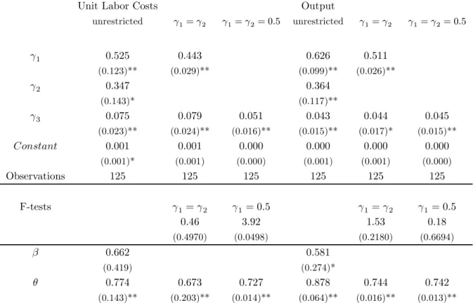
The results from estimating equation (11) by OLS are reported in table 8.23 The second and fifth column show the unrestricted estimates using unit labor costs and output, respectively, as measures for marginal costs. All coe!cients have the predicted sign and are significant.

The structural parametersandcan be retrieved using= 2

₁ together with the definition of

₃. Their values are reported in the last two rows of the table. Due to the collinearity between lagged inflation and expected future inflation, the estimates of the discount factor are rather imprecise. The implied values for the degree of price stickiness seem slightly higher than those reported in table 4 but the dierence is not significant.

For a discount factor close to one, model (11) implies₁=₂. Columns three and six of table 8 report the results of estimating equation (11) when imposing this restriction. For both specifications F-tests do not reject the equality of ₁ and₂. This contrasts to the results reported by Galí and Gertler (1999) who estimated equation (11) under the assumption of rational expectations.24 _{For all}

specifications reported in table 2 of their paper, equality of the two coe!cients would be rejected. This suggests that the indexation model performs somewhat better when survey expectations are used as a proxy for agents’ inflation expectations.

The more stringent restriction₁=₂= 1₂, however, tends to be rejected when using unit labor costs as the marginal cost measure, see column four of table 8, while it is not rejected for the case of output, see column seven.

Overall, the estimated coe!cients of equation (11) have the correct sign and the restrictions implied by theory tend not to be rejected. Although one may interpret this as cautious evidence in favor of the indexation model, the performance depends on the measure of marginal costs used. This leaves doubts on whether the indexation model is able to oer an appropriate explanation for the role of lagged inflation.

7

Conclusions

In this paper we studied the ability of the New Keynesian Phillips Curve to explain the U.S. inflation experience once the assumption of rational inflation expectations is relaxed.

The data gave considerable support for the parameter restrictions implied by the standard forward-looking New Keynesian Phillips Curve. In particular, the discount factor was found to be close to one, inflation was positively aected by real marginal costs, and the degree of price stickiness implied by the estimates suggested that about one forth of firms reset price every quarter. These results were found to be independent from whether unit labor cost or detrended output were used as a measure for real marginal costs.

Despite the generally supportive evidence, we showed that lagged inflation seems to be a sig-nificant determinant of inflation dynamics, even when taking care of potential non-rationalities in

2 3_{We also used IV estimation with two lags of expected inflation, and 4 lags of marginal costs as instruments. The}

results are very similar to the ones reported in table 8.

2 4_{These authors gave a dierent economic interpretation to equation (11): lagged inflation was supposed to enter}

inflation expectations through the use of survey expectations. The standard New Keynesian Phillips Curve cannot account for this finding.

When estimating the indexation model suggested by Christiano, Eichenbaum, and Evans (2001), which introduces an explicit role for lagged inflation, we find that output data tends to support the implied parameter restrictions while the specification tends to be rejected when using unit labor costs.

Although uncertainty remains about the role of lagged inflation, the results presented in this paper show that the New Keynesian Phillips Curve oers an empirically plausible explanation of inflation dynamics as a function of output dynamics or unit labor costs once inflation expectations are approximated with survey data.

8

Appendix

8.1

Subjective expectation and the NKPC

Here we show how one can derive the NKPC (6) with subjective expectations. Subtracting equation (1) from the same equation shifted one period forward delivers

t+1= (1)t+1+t (12) where _t+1= 1 I X i _t+1,i = 1 I X i (p,i t+1pt,i)

Applying the operatorF_t(as defined in equation (7)) to equation (12) gives

Ft[t+1] = (1)Ft£t+1¤+t (13)

Next, we express the average expectationF_t£_t+1¤in terms of expectations of observable variables. Consider the expectation of a single firm

Fi t£t+1¤=1_IFti " _I X h=1 p,h t+1pt,h # =(1_I)Fi t " _I X h=1 Ã Fh t+1 "₄ X s=0 (₎s_mct+1+s # _Fth "₄ X s=0 (₎s_mct+s #!#

where we used the first order condition (3) to obtain the second line. From this result,

Fi t£t+1¤=(1_I)Fti " _I X h=1 Fh t+1 " (1) Ã₄ X s=0 ()smct+1+s !# mct # = (1) Ã Fi t " 1 I I X h=1 p,h t+1 # mct ! = (1) µ Fi t · pt+1pt 1 ¸ mct ¶ = (1) µ 1 (1)F i t[t+1]rmct ¶

where we use condition 1 to obtain the first , the first order condition to obtain the second, pt+1= (1)1_IPI_h=1p_t+1,h +p_t to obtain the third, and mc_t=rmc_t+p_t to obtain the last line. Using this result one obtains an expression for the average expectations

Ft£t+1¤= (1) Ã 1 1 1 I I X i=1 Fi t[t+1]rmct ! (14) Substituting (14) into (13) delivers (6).

8.2

The data sources

Below we describe the data sources and the data definitions used in the paper:

Actual Inflation: is constructed using the quarterly nominal and real GDP (GNP prior to 1992)

from theReal Time Data-Set for Macroeconomists, quarters: 1968:4-2000:1, Federal Reserve Bank of Philadelphia http://www.phil.frb.org/. More details can be found in Croushore and Stark (2001).

Consumer Price Index: is the CPI for All Urban Consumer, as issued by the Bureau of Labor

Statistics. This monthly series is seasonally adjusted and downloadable via ftp from the Bureau of Labor Statistics (ftp://ftp.bls.gov/pub/time.series/cu/). Quarterly data are obtained by averaging the monthly inflation rates of the considered quarter.

Expected Inflation: is constructed using the inflation rate implied by the quarterly forecast of

the implicit GDP price deflator (GNP price deflator prior to 1992) from theSurvey of Professional

Forecasters and the actual value of the current implicit GDP deflator (GNP deflator prior to 1992),

quarters: 1968:4-2000:1, Federal Reserve Bank of Philadelphia http://www.phil.frb.org/.

Unit Labor Costs: are the log of the labor income share expressed in terms of deviation from

the sample average, where the labor income share is total compensation of employees divided by nominal GDP. The latter series are obtained from the National Income and Products Accounts Tables (Table 1.1 and Table 1.14, respectively), Quarters: 1968:4-2000:1, Bureau of Economic Analysis http://www.bea.gov/bea/dn/nipaweb/.

Output: is constructed using the quarterly real GDP (GNP prior to 1992) series from the Real

Time Data-Set for Macroeconomists, quarters: 1968:4-2000:1, Federal Reserve Bank of Philadelphia

http://www.phil.frb.org/. The series are Hodrick-Prescott filtered with smoothing parameter equal to 1600.

References

Blinder, Alan, Elie Canetti, David Lebow, and Jeremy Rudd,Asking About Prices: A New

Approach to Understanding Price Stickiness, New York: Russell Sage Foundation, 1998.

Calvo, Guillermo A., “Staggered Contracts in a Utility-Maximizing Framework,” Journal of

Monetary Economics, 1983,12, 383—398.

Christiano, Lawrence J., Martin Eichenbaum, and Charles Evans, “Nominal Rigidities and the Dynamic Eects of a Shock to Monetary Policy,”Northwestern University, 2001.

Croushore, Dean, “Introducing: The Survey of Professional Forecasters,”Federal Reserve Bank

of Philadephia Business Review, 1993, pp. 3—13.

, “Inflation Forecasts: How Good are They?,”Federal Reserve Bank of Philadelphia Business

and Tom Stark, “A Real-Time Data Set for Macroeconomists,” Journal of Econometrics, 2001,111-130, 105.

Fuhrer, Jeand George Moore, “Inflation Persistence,”Quarterly Journal of Economics, 1995,

110, 127—159.

Galí, Jordi and Mark Gertler, “Inflation Dynamics: A Structural Econometric Analysis,”

Jour-nal of Monetary Economics, 1999,44, 195—222.

Pagan, Adrian, “Econometric Issues in the Analysis of Regressions with Generated Regressors,”

International Economic Review, 1984,25, 221—247.

Roberts, John M., “New Keynesian Economics and the Phillips Curve,”Journal of Money, Credit

and Banking, 1995,27, 975—984.

, “Is Inflation Sticky?,”Journal of Monetary Economics, 1997,39, 173—196.

Rotemberg, Julio J., “Sticky Prices in the United States,” Journal of Political Economy, 1982,

60, 1187—1211.

Rudd, Jeremy and Karl Whelan, “New Tests of the New Keynesian Phillips Curve,” Federal

Reserve Board, FEDS 2001-30, 2001.

and , “Does the Labor Share of Income Drive Inflation?,”Federal Reserve Board, FEDS

2002-30, 2002.

Sbordone, Argia, “Prices and Unit Labor Costs: A New Test of Price Stickiness,” Journal of

Monetary Economics, 2002,49, 265—292.

Woodford, Michael, “Imperfect Common Knowledge and the Eects of Monetary Policy,”

9

Figures and Tables

1968:4

1974:4

1980:4

1986:4

1992:4

1998:4

0

.05

.1

.15

Solid line: expected inflation; dashed line: actual inflation.

1968:4

1974:4

1980:4

1986:4

1992:4

1998:4

-.2

-.1

0

.1

.2

Solid line: unit labor costs (the log of compensation of employees divided by GDP in deviation from the sample mean); dashed line: Hodrick-Prescott (1600) filtered output.

Lag

-20

-10

0

10

20

-1

-.75

-.5

-.25

0

.25

.5

.75

1

Lag

-20

-10

0

10

20

-1

-.75

-.5

-.25

0

.25

.5

.75

1

Table 1: Biasedness of expectations Constant 0.005 (0.001)** Dummy(1968 : 41979 : 4) -0.016 (0.003)** Dummy(1980 : 11989 : 4) 0.008 (0.002)** Observations 126 R-squared 0.32

Note: The dependent variable is the inflation forecast error. In column two forecast errors are regressed on a constant; in column three forecast errors are regressed on a constant and two time dummies. Asymptotic Newey-West 4 lags standard errors are reported in parentheses. One (two) star(s) indicate significance at the 5% (1%) level.

Table 2: The structure of forecast errors

Constant 0.000 0.005 (0.002) (0.001)** ₁ 0.547 0.335 (0.083)** (0.095)** Dummy(1968 : 41979 : 4) -0.016 (0.003)** Dummy(1980 : 11989 : 4) 0.001 (0.002) Observations 126 126

Note: The dependent variable is the inflation forecast error. The second column fits an AR(1) and reports the AR-coe!cient; the third column adds two time dummies; the forth column adds a fourth-order moving average to capture potential seasonalities. Asymptotic standard errors are reported in parentheses. One (two) star(s) indicate significance at the 5% (1%) level.

Table 3: Orthogonality tests

F-statistics

Output Inflation Unit Labor Costs CP I Inflation All

Lags 1-4 4.48 6.56 6.81 3.34 3.68 (0.0021) (0.0001) (0.0001) (0.0126) (0.0001) Observations 122 122 122 122 122 R-squared 0.13 0.18 0.19 0.15 0.26 Lags 2-4 5.85 2.40 3.57 3.96 3.47 ( 0.0009) (0.0715) (0.0163) (0.0099) (0.0002) Observations 122 122 122 122 122 R-squared 0.11 0.03 0.06 0.07 0.19

Note: The inflation forecast error is regressed on lags 1 to 4 (top panel) and 2 to 4 (bottom panel) of output, inflation, unit labor costs, CPI inflation, and on all of these variables in the row named ’All’. The table reports F-statistics for the hypothesis that the coe!cients on all included regressors are jointly equal to zero wit p-values in parentheses.

Table 4: The New Keynesian Phillips Curve

Unit Labor Costs Output

unrestricted q= 1 unrestricted q= 1 0.990 1 1.018 1 (0.035)** - (0.041)** 0.098 0.096 0.055 0.055 (0.027)** (0.018)** (0.026)** (0.018)** 0.735 0.734 0.785 0.791 (0.037)** (0.022)** (0.050)** (0.030)** Observations 126 126 126 126

Note: The dependent variable is actual inflation. In the second and third column it is regressed on expected inflation and unit labor costs, in the forth and fifth column on expected inflation and output. The coe!cientsqandbdenote the discount factor and the coe!cient attached to marginal costs. In the third and fifth column q is constrained to be equal to one. The value of the stickiness parameterw is calculated using the point estimates ofq and b. Asymptotic Newey-West 4 lags standard errors are reported in parentheses. One (two) star(s) indicate significance at the 5% (1%) level.

Table 5: Sub-Sample Stability

Unit Labor Costs Output

1968:4-1979:4 1.0140 0.2097 0.6316 1.1512 0.0547 0.7361 (0.0524)** (0.0407)** (0.0367)** (0.0596)** (0.0210)* (0.0674)** 1980:1-1989:4 0.8541 0.0962 0.7774 0.8949 0.0170 0.9144 (0.0257)** (0.0425)* (0.0750)** (0.0484)** (0.0267) (0.0747)** 1990:1-2000:1 0.8627 0.0149 0.9297 0.8527 0.0792 0.8004 (0.0499)** (0.0311) (0.0774)** (0.0362)** (0.0573) (0.0459)** Note: The coe!cientsq, b andw denote the discount factor, the coe!cient attached to real marginal costs, and the degree of price stickiness, respectively. Columns two to four use unit labor costs while columns five to seven use detrended output. Asymptotic Newey-West 4 lags standard errors are reported in parentheses. One (two) star(s) indicate significancy at the 5%(1%) level.

Table 6: The Role of Lagged Variables

Unit Labor Costs Output

0.445 1.153 0.990 0.376 1.089 1.015 (0.124)** (0.183)** (0.036)** (0.094)** (0.214)** (0.039)** 0.050 0.097 0.120 0.042 0.053 0.009 (0.019)** (0.026)** (0.060)* (0.015)** (0.027) (0.042) t1 0.543 0.623 (0.124)** (0.096)** Et1[t] -0.165 -0.072 (0.173) (0.198) rmct1 -0.024 0.053 (0.049) (0.043) Observations 125 125 125 125 125 125

Note: The dependent variable is actual inflation, which is regressed on expected inflation (q) and marginal costs (b). In columns two to four (five to seven) marginal costs are given by unit labor costs (detrended output). As additional regressors enter lagged inflation (columns two and five), lagged expected inflation (columns three and six) and lagged marginal costs (columns four and seven). Asymptotic Newey-West 4 lags standard errors are reported in parentheses. One (two) star(s) indicate significance at the 5% (1%) level.

Table 7: Lagged Inflation

Unit Labor Costs Output

1.000 1.018 (0.024)** (0.023)** 0.061 0.044 (0.017)** (0.014)** orthogonalized inflation(t1) 0.548 0.625 (0.121)** (0.101)** 0.782 0.805 (0.0310)** (0.031)** Observations 125 125

Note: The dependent variable is actual inflation, which is regressed on expected inflation (q) and real marginal costs (b), given by unit labor costs in the second column and detrended output in the third column. As additional regressor enters orthogonalized inflation which are the residuals obtained from regressing the timetinflation expectations on actualt31inflation. The value of the stickiness parameter w is calculated using the point estimates of q and b. Asymptotic Newey-West 4 lags standard errors are reported in parentheses. One (two) star(s) indicate significance at the 5% (1%) level.

Table 8: The Indexation Model

Unit Labor Costs Output

unrestricted ₁=_{2 1}=₂= 0.5 unrestricted ₁=_{2 1}=₂= 0.5 ₁ 0.525 0.443 0.626 0.511 (0.123)** (0.029)** (0.099)** (0.026)** ₂ 0.347 0.364 (0.143)* (0.117)** ₃ 0.075 0.079 0.051 0.043 0.044 0.045 (0.023)** (0.024)** (0.016)** (0.015)** (0.017)* (0.015)** Constant 0.001 0.001 0.000 0.000 0.000 0.000 (0.001)* (0.001) (0.000) (0.001) (0.001) (0.000) Observations 125 125 125 125 125 125 F-tests ₁=_{2 1}= 0.5 ₁=_{2 1}= 0.5 0.46 3.92 1.53 0.18 (0.4970) (0.0498) (0.2180) (0.6694) 0.662 0.581 (0.419) (0.274)* 0.774 0.673 0.727 0.878 0.744 0.742 (0.143)** (0.203)** (0.014)** (0.064)** (0.016)** (0.013)** Note: The dependent variable is actual inflation, which is regressed on lagged inflation (₁), expected inflation (₂), and real marginal costs (₃), where the latter are given by unit labor costs (detrended output) in columns two to four (five to seven). Columns two and five report unrestricted estimates; columns three and six constrain ₁ and ₂ to be equal; columns four and seven restrict ₁ and₂ to be equal to0.5. Successive F-tests for these restrictions with p-values in parentheses are reported in the respective columns. The values ofqandwreported are the ones implied by the point estimates of₁,₂, and₃. Asymptotic Newey-West 4 lags standard errors are reported in parentheses. One (two) star(s) indicate significance at the 5% (1%) level.

(XURSHDQ&HQWUDO%DQNZRUNLQJSDSHUVHULHV

)RUDFRPSOHWHOLVWRI:RUNLQJ3DSHUVSXEOLVKHGE\WKH(&%SOHDVHYLVLWWKH(&%·VZHEVLWH KWWSZZZHFELQW ´)LQDQFLDOIULFWLRQVDQGWKHPRQHWDU\WUDQVPLVVLRQPHFKDQLVPWKHRU\HYLGHQFHDQGSROLF\ LPSOLFDWLRQVµE\&%HDQ-/DUVHQDQG.1LNRORY-DQXDU\ ´0RQHWDU\WUDQVPLVVLRQLQWKHHXURDUHDZKHUHGRZHVWDQG"µE\,$QJHORQL$.DVK\DS %0RMRQ'7HUOL]]HVH-DQXDU\ ´0RQHWDU\SROLF\UXOHVPDFURHFRQRPLFVWDELOLW\DQGLQIODWLRQDYLHZIURPWKHWUHQFKHVµ E\$2USKDQLGHV'HFHPEHU ´5HQWLQGLFHVIRUKRXVLQJLQ:HVW*HUPDQ\WRµE\-+RIIPDQQDQG&.XU] -DQXDU\ ´+HGRQLFKRXVHSULFHVZLWKRXWFKDUDFWHULVWLFVWKHFDVHRIQHZPXOWLXQLWKRXVLQJµE\ 2%RYHUDQG39HOLOOD-DQXDU\ ´'XUDEOHJRRGVSULFHLQGH[HVDQGTXDOLW\FKDQJHDQDSSOLFDWLRQWRDXWRPRELOHSULFHVLQ ,WDO\µE\*07RPDW-DQXDU\ ´0RQHWDU\SROLF\DQGWKHVWRFNPDUNHWLQWKHHXURDUHDµE\1&DVVRODDQG&0RUDQD -DQXDU\ ´/HDUQLQJVWDELOLW\LQHFRQRPLFVZLWKKHWHURJHQRXVDJHQWVµE\6+RQNDSRKMDDQG.0LWUD -DQXDU\ ´1DWXUDOUDWHGRXEWVµE\$%H\HUDQG5($)DUPHU)HEUXDU\ ´1HZWHFKQRORJLHVDQGSURGXFWLYLW\JURZWKLQWKHHXURDUHDµE\)9LMVHODDUDQG5$OEHUV )HEUXDU\ ´$QDO\VLQJDQGFRPELQLQJPXOWLSOHFUHGLWDVVHVVPHQWVRIILQDQFLDOLQVWLWXWLRQVµE\(7DEDNLV DQG$9LQFL)HEUXDU\ ´0RQHWDU\SROLF\H[SHFWDWLRQVDQGFRPPLWPHQWµE\*:(YDQVDQG6+RQNDSRKMD )HEUXDU\ ´'XUDWLRQYROXPHDQGYRODWLOLW\LPSDFWRIWUDGHVµE\60DQJDQHOOL)HEUXDU\ ´2SWLPDOFRQWUDFWVLQDG\QDPLFFRVWO\VWDWHYHULILFDWLRQPRGHOµE\&0RQQHWDQG (4XLQWLQ)HEUXDU\ ´3HUIRUPDQFHRIPRQHWDU\SROLF\ZLWKLQWHUQDOFHQWUDOEDQNIRUHFDVWLQJµE\6+RQNDSRKMD DQG.0LWUD)HEUXDU\

´1RQVWDQGDUGFHQWUDOEDQNORVVIXQFWLRQVVNHZHGULVNVDQGFHUWDLQW\HTXLYDOHQFHµE\ $DO1RZDLKLDQG/6WUDFFD0DUFK ´+DUPRQL]HGLQGH[HVRIFRQVXPHUSULFHVWKHLUFRQFHSWXDOIRXQGDWLRQVµE\('LHZHUW 0DUFK ´0HDVXUHPHQWELDVLQWKH+,&3ZKDWGRZHNQRZDQGZKDWGRZHQHHGWRNQRZ"µE\ 0$:\QQHDQG'5RGUtJXH]3DOHQ]XHOD0DUFK ´,QIODWLRQG\QDPLFVDQGGXDOLQIODWLRQLQDFFHVVLRQFRXQWULHVD´QHZ.H\QHVLDQµ SHUVSHFWLYHµE\2$UUDWLEHO'5RGUtJXH]3DOHQ]XHODDQG&7KLPDQQ0DUFK ´&DQFRQILGHQFHLQGLFDWRUVEHXVHIXOWRSUHGLFWVKRUWWHUPUHDO*'3JURZWK"µE\ $0RXURXJDQHDQG05RPD0DUFK ´7KHFRVWRISULYDWHWUDQVSRUWDWLRQLQWKH1HWKHUODQGVµE\%%RGHDQG -9DQ'DOHQ0DUFK ´7KHRSWLPDOPL[RIWD[HVRQPRQH\FRQVXPSWLRQDQGLQFRPHµE\)'H)LRUHDQG 37HOHV$SULO ´5HWDLOEDQNLQWHUHVWUDWHSDVVWKURXJKWKHQHZHYLGHQFHDWWKHHXURDUHDOHYHOµE\ *GH%RQGW$SULO ´(TXLOLEULXPELGGLQJLQWKHHXURV\VWHP·VRSHQPDUNHWRSHUDWLRQVµE\8%LQGVHLO$SULO ´1HZµYLHZVRQWKHRSWLPXPFXUUHQF\DUHDWKHRU\ZKDWLV(08WHOOLQJXV"µE\ )30RQJHOOL$SULO ´2QFXUUHQF\FULVHVDQGFRQWDJLRQµE\0)UDW]VFKHU$SULO ´3ULFHVHWWLQJDQGWKHVWHDG\VWDWHHIIHFWVRILQIODWLRQµE\0&DVDUHV0D\ ´$VVHWSULFHVDQGILVFDOEDODQFHVµE\)(VFKHQEDFKDQG/6FKXNQHFKW0D\ ´0RGHOOLQJWKHGDLO\EDQNQRWHVLQFLUFXODWLRQLQWKHFRQWH[WRIWKHOLTXLGLW\PDQDJHPHQWRI WKH(XURSHDQ&HQWUDO%DQNµE\$&DEUHUR*&DPED0HQGH]$+LUVFKDQG)1LHWR 0D\ ´$QRQSDUDPHWULFPHWKRGIRUYDOXLQJQHZJRRGVµE\,&UDZIRUG0D\ ´$IDLOXUHLQWKHPHDVXUHPHQWRILQIODWLRQUHVXOWVIURPDKHGRQLFDQGPDWFKHGH[SHULPHQW XVLQJVFDQQHUGDWDµE\06LOYHUDQG6+HUDYL0D\ ´7RZDUGVDQHZHDUO\ZDUQLQJV\VWHPRIILQDQFLDOFULVHVµE\0)UDW]VFKHUDQG0%XVVLHUH 0D\

´7LPHWREXLOGDSSURDFKLQDVWLFN\SULFHVWULFN\ZDJHRSWLPL]LQJPRQHWDU\PRGHOE\ 0&DVDUHV0D\ ´7KHIXQFWLRQDOIRUPRI\LHOGFXUYHVµE\9%URXVVHDX0D\ ´7KH6SDQLVKEORFNRIWKH(6&%PXOWLFRXQWU\PRGHOµE\$(VWUDGDDQG$:LOOPDQ0D\ ´(TXLW\DQGERQGPDUNHWVLJQDOVDVOHDGLQJLQGLFDWRUVRIEDQNIUDJLOLW\µE\5*URSS -9HVDODDQG*9XOSHV-XQH ´*LQIODWLRQIRUHFDVWVµE\)&DQRYD-XQH ´6KRUWWHUPPRQLWRULQJRIILVFDOSROLF\GLVFLSOLQHµE\*&DPED0HQGH]DQG$/DPR-XQH ´(XURDUHDSURGXFWLRQIXQFWLRQDQGSRWHQWLDORXWSXWDVXSSO\VLGHV\VWHPDSSURDFKµE\ $:LOOPDQ-XQH ´7KHHXUREORFWKHGROODUEORFDQGWKH\HQEORFKRZPXFKPRQHWDU\SROLF\LQGHSHQGHQFH FDQH[FKDQJHUDWHIOH[LELOLW\EX\LQDQLQWHUGHSHQGHQWZRUOG"µE\0)UDW]VFKHU-XQH ´<RXWKXQHPSOR\PHQWLQWKH2(&'GHPRJUDSKLFVKLIWVODERXUPDUNHWLQVWLWXWLRQVDQG PDFURHFRQRPLFVKRFNVµE\-)-LPHQRDQG'5RGULJXH]3DOHQ]XHOD-XQH ´,GHQWLI\LQJHQGRJHQRXVILVFDOSROLF\UXOHVIRUPDFURHFRQRPLFPRGHOVµE\--3HUH] DQG3+LHEHUW-XO\ ´%LGGLQJDQGSHUIRUPDQFHLQUHSRDXFWLRQVHYLGHQFHIURP(&%RSHQPDUNHWRSHUDWLRQVµ E\.*1\ERUJ8%LQGVHLODQG,$6WUHEXODHY-XO\ ´4XDQWLI\LQJ(PERGLHG7HFKQRORJLFDO&KDQJHµE\36DNHOODULVDQG'-:LOVRQ-XO\ ´2SWLPDOSXEOLFPRQH\µE\&0RQQHW-XO\ ´0RGHOXQFHUWDLQW\DQGWKHHTXLOLEULXPYDOXHRIWKHUHDOHIIHFWLYHHXURH[FKDQJHUDWHµE\ &'HWNHQ$'LHSSH-+HQU\&0DULQDQG)6PHWV-XO\ ´7KHRSWLPDODOORFDWLRQRIULVNVXQGHUSURVSHFWWKHRU\µE\/6WUDFFD-XO\ ´3XEOLFGHEWDV\PPHWULHVWKHHIIHFWRQWD[HVDQGVSHQGLQJLQWKH(XURSHDQ8QLRQµE\ 6.URJVWUXS$XJXVW ´7KHUDWLRQDOLW\RIFRQVXPHUV·LQIODWLRQH[SHFWDWLRQVVXUYH\EDVHGHYLGHQFHIRUWKHHXUR DUHDµE\0)RUVHOOVDQG*.HQQ\$XJXVW ´(XURDUHDFRUSRUDWHGHEWVHFXULWLHVPDUNHWILUVWHPSLULFDOHYLGHQFHµE\*GH%RQGW $XJXVW

´7KHLQGXVWU\HIIHFWVRIPRQHWDU\SROLF\LQWKHHXURDUHDµE\*3HHUVPDQDQG)6PHWV $XJXVW ´0RQHWDU\DQGILVFDOSROLF\LQWHUDFWLRQVLQDPLFURIRXQGHGPRGHORIDPRQHWDU\XQLRQµE\ 50:-%HHWVPDDQG+-HQVHQ$XJXVW ´,GHQWLI\LQJWKHHIIHFWVRIPRQHWDU\SROLF\VKRFNVRQH[FKDQJHUDWHVXVLQJKLJKIUHTXHQF\ GDWDE\-)DXVW-+5RJHUV(6ZDQVRQDQG-+:ULJKW$XJXVW ´(VWLPDWLQJWKHHIIHFWVRIILVFDOSROLF\LQ2(&'FRXQWULHVµE\53HURWWL$XJXVW ´0RGHOLQJPRGHOXQFHUWDLQW\µE\$2QDWVNLDQG1:LOOLDPV$XJXVW ´:KDWPHDVXUHRILQIODWLRQVKRXOGDFHQWUDOEDQNWDUJHW"µE\*0DQNLZDQG55HLV $XJXVW ´$QHVWLPDWHGVWRFKDVWLFG\QDPLFJHQHUDOHTXLOLEULXPPRGHORIWKHHXURDUHDµE\)6PHWV DQG5:RXWHUV$XJXVW ´&RQVWUXFWLQJTXDOLW\DGMXVWHGSULFHLQGLFHVDFRPSDULVRQRIKHGRQLFDQGGLVFUHWHFKRLFH PRGHOVµE\1-RQNHU6HSWHPEHU ´2SHQQHVVDQGHTXLOLEULXPGHWHUPLQDF\XQGHULQWHUHVWUDWHUXOHVµE\)GH)LRUHDQG =/LX6HSWHPEHU ´,QWHUQDWLRQDOPRQHWDU\SROLF\FRRUGLQDWLRQDQGILQDQFLDOPDUNHWLQWHJUDWLRQµE\ $6XWKHUODQG6HSWHPEHU ´0RQHWDU\SROLF\DQGWKHILQDQFLDODFFHOHUDWRULQDPRQHWDU\XQLRQµE\6*LOFKULVW -2+DLUDXOWDQG+.HPSI6HSWHPEHU ´0DFURHFRQRPLFVRILQWHUQDWLRQDOSULFHGLVFULPLQDWLRQµE\*&RUVHWWLDQG/'HGROD 6HSWHPEHU ´$WKHRU\RIWKHFXUUHQF\GHQRPLQDWLRQRILQWHUQDWLRQDOWUDGHµE\3%DFFKHWWDDQG (YDQ:LQFRRS6HSWHPEHU ´,QIODWLRQSHUVLVWHQFHDQGRSWLPDOPRQHWDU\SROLF\LQWKHHXURDUHDµE\3%HQLJQRDQG -'/ySH]6DOLGR6HSWHPEHU ´2SWLPDOPRQHWDU\SROLF\ZLWKGXUDEOHDQGQRQGXUDEOHJRRGVµE\&-(UFHJDQG $7/HYLQ6HSWHPEHU ´5HJLRQDOLQIODWLRQLQDFXUUHQF\XQLRQILVFDOSROLF\YVIXQGDPHQWDOVµE\0'XDUWHDQG $/:ROPDQ6HSWHPEHU ´,QIODWLRQG\QDPLFVDQGLQWHUQDWLRQDOOLQNDJHVDPRGHORIWKH8QLWHG6WDWHVWKHHXURDUHD DQG-DSDQµE\*&RHQHQDQG9:LHODQG6HSWHPEHU

´0RQHWDU\SROLF\LQDZRUOGZLWKGLIIHUHQWILQDQFLDOV\VWHPVµE\()DLD2FWREHU ´(IILFLHQWSULFLQJRIODUJHYDOXHLQWHUEDQNSD\PHQWV\VWHPVµE\&+ROWKDXVHQDQG -&5RFKHW2FWREHU ´(XURSHDQLQWHJUDWLRQZKDWOHVVRQVIRURWKHUUHJLRQV"7KHFDVHRI/DWLQ$PHULFDµE\ ('RUUXFFL6)LUSR0)UDW]VFKHUDQG)30RQJHOOL2FWREHU ´8VLQJPRQH\PDUNHWUDWHVWRDVVHVVWKHDOWHUQDWLYHVRIIL[HGYVYDULDEOHUDWHWHQGHUVWKH OHVVRQIURPGDWDIRU*HUPDQ\µE\00DQQD2FWREHU ´$ILVFDOWKHRU\RIVRYHUHLJQULVNµE\08ULEH2FWREHU ´6KRXOGFHQWUDOEDQNVUHDOO\EHIOH[LEOH"µE\+3*UQHU2FWREHU ´'HEWUHGXFWLRQDQGDXWRPDWLFVWDELOLVDWLRQµE\3+LHEHUW--3pUH]DQG05RVWDJQR 2FWREHU ´0RQHWDU\SROLF\DQGWKH]HURERXQGWRLQWHUHVWUDWHVDUHYLHZµE\7<DWHV2FWREHU ´7KHILVFDOFRVWVRIILQDQFLDOLQVWDELOLW\UHYLVLWHGµE\/6FKXNQHFKWDQG)(VFKHQEDFK 1RYHPEHU ´,VWKH(XURSHDQ&HQWUDO%DQNDQGWKH8QLWHG6WDWHV)HGHUDO5HVHUYHSUHGLFWDEOH"µE\ *3HUH]4XLURVDQG-6LFLOLD1RYHPEHU ´6XVWDLQDELOLW\RISXEOLFILQDQFHVDQGDXWRPDWLFVWDELOLVDWLRQXQGHUDUXOHRIEXGJHWDU\ GLVFLSOLQHµE\-0DUtQ1RYHPEHU ´6HQVLWLYLW\DQDO\VLVRIYRODWLOLW\DQHZWRROIRUULVNPDQDJHPHQWµE\60DQJDQHOOL9&HFL DQG:9HFFKLDWR1RYHPEHU ´,QVDPSOHRURXWRIVDPSOHWHVWVRISUHGLFWDELOLW\ZKLFKRQHVKRXOGZHXVH"µE\$,QRXH DQG/.LOLDQ1RYHPEHU ´%RRWVWUDSSLQJDXWRUHJUHVVLRQVZLWKFRQGLWLRQDOKHWHURVNHGDVWLFLW\RIXQNQRZQIRUPµE\ 6*RQoDOYHVDQG/.LOLDQ1RYHPEHU ´$PRGHORIWKH(XURV\VWHP·VRSHUDWLRQDOIUDPHZRUNIRUPRQHWDU\SROLF\LPSOHPHQWDWLRQµ E\&(ZHUKDUW1RYHPEHU ´([WUDFWLQJULVNQHXWUDOSUREDELOLW\GHQVLWLHVE\ILWWLQJLPSOLHGYRODWLOLW\VPLOHVVRPH PHWKRGRORJLFDOSRLQWVDQGDQDSSOLFDWLRQWRWKH0(XULERUIXWXUHVRSWLRQSULFHVµE\ $%$QGHUVHQDQG7:DJHQHU'HFHPEHU ´7LPHYDULDWLRQLQWKHWDLOEHKDYLRXURIEXQGIXWXUHVUHWXUQVµE\7:HUQHUDQG&8SSHU 'HFHPEHU

´,QWHUGHSHQGHQFHEHWZHHQWKHHXURDUHDDQGWKH86ZKDWUROHIRU(08"µE\0(KUPDQQ DQG0)UDW]VFKHU'HFHPEHU ´(XURDUHDLQIODWLRQSHUVLVWHQFHµE\1%DWLQL'HFHPEHU ´$JJUHJDWHORDQVWRWKHHXURDUHDSULYDWHVHFWRUµE\$&DO]D00DQULTXHDQG-6RXVD -DQXDU\ ´0\RSLFORVVDYHUVLRQGLVDSSRLQWPHQWDYHUVLRQDQGWKHHTXLW\SUHPLXPSX]]OHµE\ ')LHOGLQJDQG/6WUDFFD-DQXDU\ ´$V\PPHWULFG\QDPLFVLQWKHFRUUHODWLRQVRIJOREDOHTXLW\DQGERQGUHWXUQVµE\ /&DSSLHOOR5)(QJOHDQG.6KHSSDUG-DQXDU\ ´5HDOH[FKDQJHUDWHLQDQLQWHUWHPSRUDOQFRXQWU\PRGHOZLWKLQFRPSOHWHPDUNHWVµE\ %0HUFHUHDX-DQXDU\ ´(PSLULFDOHVWLPDWHVRIUHDFWLRQIXQFWLRQVIRUWKHHXURDUHDµE\'*HUGHVPHLHUDQG %5RIILD-DQXDU\ ´$FRPSUHKHQVLYHPRGHORQWKHHXURRYHUQLJKWUDWHµE\)5:UW]-DQXDU\ ´'RGHPRJUDSKLFFKDQJHVDIIHFWULVNSUHPLXPV"(YLGHQFHIURPLQWHUQDWLRQDOGDWDµE\ $$QJDQG$0DGGDORQL-DQXDU\ ´$IUDPHZRUNIRUFROODWHUDOULVNFRQWUROGHWHUPLQDWLRQµE\'&RVVLQ=+XDQJ '$XQRQ1HULQDQG)*RQ]iOH]-DQXDU\ ´$QWLFLSDWHG5DPVH\UHIRUPVDQGWKHXQLIRUPWD[DWLRQSULQFLSOHWKHUROHRILQWHUQDWLRQDO ILQDQFLDOPDUNHWVµE\66FKPLWW*URKpDQG08ULEH-DQXDU\ ´6HOIFRQWURODQGVDYLQJVµE\30LFKHODQG-39LGDO-DQXDU\ ´0RGHOOLQJWKHLPSOLHGSUREDELOLW\RIVWRFNPDUNHWPRYHPHQWVµE\(*ODW]HUDQG 06FKHLFKHU-DQXDU\ ´$JJUHJDWLRQDQGHXURDUHD3KLOOLSVFXUYHVµE\6)DELDQLDQG-0RUJDQ)HEUXDU\ ´2QWKHVHOHFWLRQRIIRUHFDVWLQJPRGHOVµE\$,QRXHDQG/.LOLDQ)HEUXDU\ ´%XGJHWLQVWLWXWLRQVDQGILVFDOSHUIRUPDQFHLQ&HQWUDODQG(DVWHUQ(XURSHDQFRXQWULHVµE\ +*OHLFK)HEUXDU\ ´7KHDGPLVVLRQRIDFFHVVLRQFRXQWULHVWRDQHQODUJHGPRQHWDU\XQLRQDWHQWDWLYH DVVHVVPHQWµE\0&D·=RU]LDQG5$'H6DQWLV)HEUXDU\ ´7KHUROHRISURGXFWPDUNHWUHJXODWLRQVLQWKHSURFHVVRIVWUXFWXUDOFKDQJHµE\-0HVVLQD 0DUFK

´([WUDHXURDUHDPDQXIDFWXULQJLPSRUWSULFHVDQGH[FKDQJHUDWHSDVVWKURXJKµE\ %$QGHUWRQ0DUFK ´7KHDOORFDWLRQRIFRPSHWHQFLHVLQDQLQWHUQDWLRQDOXQLRQDSRVLWLYHDQDO\VLVµE\05XWD $SULO ´(VWLPDWLQJULVNSUHPLDLQPRQH\PDUNHWUDWHVµE\$'XUUp6(YMHQDQG53LOHJDDUG $SULO ´,QIODWLRQG\QDPLFVDQGVXEMHFWLYHH[SHFWDWLRQVLQWKH8QLWHG6WDWHVµE\.$GDPDQG 03DGXOD$SULO