OPTIMIZATION AND CONTROL

(1)

OPTIMIZATION AND CONTROL

Richard Weber

Schedules

The first 6 lectures are devoted to dynamic programming in discrete-time and cover both finite and infinite-horizon problems; discounted-cost, positive, negative and average-cost programming; the time-homogeneous Markov case; stopping problems; value iteration and policy improvement.

The next 5 lectures are devoted to theLQG model(linear systems, quadratic costs) and cover the important ideas of controllability and observability; the Ricatti equation; imperfect observation, certainly equivalence and the Kalman filter.

The final 5 lectures are devoted tocontinuous-time modelsand include treatment of Pontryagin’s maximum principle and the Hamiltonian; Markov decision processes on a countable state space and controlled diffusion processes.

Each of the 16 lectures is designed to be a somewhat self-contained unit, e.g., there will be one lecture on ‘Negative Programming’, one on ‘Controllability’, etc. Examples and applications are important in this course, so there are one or more worked examples in each lecture.

Examples sheets

There are three examples sheets, corresponding to the thirds of the course. There are two or three questions for each lecture, some theoretical and some of a problem nature. Each question is marked to indicate the lecture with which it is associated.

Lecture Notes and Handouts

There are printed lecture notes for the course and other occasional handouts. There are sheets summarising notation and what you are expected to know for the exams.

The notes include a list of keywords and I will be drawing your attention to these as we go along. If you have a good grasp of the meaning of each of these keywords, then you will be well on your way to understanding the important concepts of the course.

WWW pages

Notes for the course, and other information are on the web at

http://www.statslab.cam.ac.uk/~rrw1/oc/index.html.

Books

The following books are recommended.

D. P. Bertsekas,Dynamic Programming, Prentice Hall, 1987. D. P. Bertsekas,Dynamic Programming and Optimal Control, Volumes I and II, Prentice Hall, 1995.

L. M. Hocking,Optimal Control: An introduction to the theory and applications, Oxford 1991.

S. Ross,Introduction to Stochastic Dynamic Programming, Academic Press, 1983. P. Whittle, Optimization Over Time. Volumes I and II, Wiley, 1982-83.

Ross’s book is probably the easiest to read. However, it only covers Part I of the course. Whittle’s book is good for Part II and Hocking’s book is good for Part III. The recent book by Bertsekas is useful for all parts. Many other books address the topics of the course and a collection can be found in Sections 3B and 3D of the DPMMS library. Notation differs from book to book. My notation will be closest to that of Whittle’s books and consistent throughout. For example, I will always denote a minimal cost function by F(·) (whereas, in the recommended books you will find F, V, φ, J and many others symbols used for this quantity.)

(3)

1 Dynamic Programming: The Optimality Equation

We introduce the idea of dynamic programming and the principle of optimality. We give notation for state-structured models, and introduce ideas of feedback, open-loop, and closed-loop controls, a Markov decision process, and the idea that it can be useful to model things in terms of time to go.

1.1 Control as optimization over time

Optimization is a key tool in modelling. Sometimes it is important to solve a prob-lem optimally. Other times either a near-optimal solution is good enough, or the real problem does not have a single criterion by which a solution can be judged. However, even then optimization is useful as a way to test thinking. If the ‘optimal’ solution is ridiculous it may suggest ways in which both modelling and thinking can be refined.

Control theory is concerned with dynamic systems and their optimization over time. It accounts for the fact that a dynamic system may evolve stochastically and that key variables may be unknown or imperfectly observed (as we see, for instance, in the UK economy).

This contrasts with optimization models in the IB course (such as those for LP and network flow models); these static and nothing was random or hidden. It is these three new features: dynamic and stochastic evolution, and imperfect state observation, that give rise to new types of optimization problem and which require new ways of thinking. We could spend an entire lecture discussing the importance of control theory and tracing its development through the windmill, steam governor, and so on. Such ‘classic control theory’ is largely concerned with the question of stability, and there is much of this theory which we ignore, e.g., Nyquist criterion and dynamic lags.

1.2 The principle of optimality

A key idea is that optimization over time can often be regarded as ‘optimization in stages’. We trade off our desire to obtain the lowest possible cost at the present stage against the implication this would have for costs at future stages. The best action minimizes the sum of the cost incurred at the current stage and the least total cost that can be incurred from all subsequent stages, consequent on this decision. This is known as the Principle of Optimality.

Definition 1.1 (Principle of Optimality) From any point on an optimal trajectory, the remaining trajectory is optimal for the corresponding problem initiated at that point.

1.3 Example: the shortest path problem

Consider the ‘stagecoach problem’ in which a traveler wishes to minimize the length of a journey from town A to town J by first traveling to one of B, C or D and then onwards to one of E, F or G then onwards to one of H or I and the finally to J. Thus there are 4 ‘stages’. The arcs are marked with distances between towns.

A B C D E F G H I J 1 1 2 2 3 3 3 3 3 3 4 4 4 4 4 4 5 6 6 7

Road system for stagecoach problem

Solution. LetF(X) be the minimal distance required to reach J from X. Then clearly,

F(J) = 0,F(H) = 3 andF(I) = 4.

F(F) = min[ 6 +F(H),3 +F(I) ] = 7,

and so on. Recursively, we obtainF(A) = 11 and simultaneously an optimal route, i.e., A_→D_→F_→I_→J (although it is not unique).

The study of dynamic programming dates from Richard Bellman, who wrote the first book on the subject (1957) and gave it its name. A very large number of problems can be treated this way.

1.4 The optimality equation

The optimality equation in the general case. Indiscrete-timet takes integer values, sayt= 0,1, . . .. Supposeutis acontrol variablewhose value is to be chosen at

timet. LetUt−1= (u0, . . . , ut−1) denote the partial sequence of controls (or decisions)

taken over the first tstages. Suppose the cost up to thetime horizonhis given by

C=G(Uh−1) =G(u0, u1, . . . , uh−1).

Then theprinciple of optimalityis expressed in the following theorem.

Theorem 1.2 (The principle of optimality) Define the functions G(Ut−1, t) = inf

ut,ut+1,...,uh−1

G(Uh−1).

Then these obey the recursion

G(Ut−1, t) = inf ut

G(Ut, t+ 1) t < h ,

with terminal evaluation G(Uh−1, h) =G(Uh−1).

The proof is immediate from the definition of G(Ut−1, t), i.e.,

G(Ut−1, t) = inf ut

inf

ut+1,...,uh−1

(4)

The state structured case. The control variableutis chosen on the basis of knowing

Ut−1 = (u0, . . . , ut−1), (which determines everything else). But a more economical

representation of the past history is often sufficient. For example, we may not need to know the entire path that has been followed up to time t, but only the place to which it has taken us. The idea of astate variablex_∈Rdis that its value att, denotedxt,

is calculable from known quantities and obeys aplant equation(or law of motion)

xt+1=a(xt, ut, t).

Suppose we wish to minimize a cost function of the form

C=

h−1

X

t=0

c(xt, ut, t) +Ch(xh), (1.1)

by choice of controls_{u0, . . . , uh−1}. Define the cost from timet onwards as, Ct=

h−1

X

τ=t

c(xτ, uτ, τ) +Ch(xh), (1.2)

and the minimal cost from timetonwards as an optimization over_{ut, . . . , uh−1}

con-ditional onxt=x,

F(x, t) = inf

ut,...,uh−1 Ct.

HereF(x, t) is the minimal future cost from timetonward, given that the state isxat timet. Then by an inductive proof, one can show as in Theorem 1.2 that

F(x, t) = inf

u [c(x, u, t) +F(a(x, u, t), t+ 1)], t < h , (1.3)

with terminal condition F(x, h) =Ch(x). Here xis a generic value of xt. The

mini-mizinguin (1.3) is the optimal controlu(x, t) and values ofx0, . . . , xt−1are irrelevant.

Theoptimality equation(1.3) is also called thedynamic programming equation

(DP) orBellman equation.

The DP equation defines an optimal control problem in what is calledfeedbackor

closed loopform, withut=u(xt, t). This is in contrast to theopen loopformulation

in which _{u0, . . . , uh−1} are to be determined all at once at time 0. A policy (or

strategy) is a rule for choosing the value of the control variable under all possible circumstances as a function of the perceived circumstances. To summarise:

(i) The optimalut is a function only ofxtandt, i.e,ut=u(xt, t).

(ii) The DP equation expresses the optimal ut in closed loop form. It is optimal

whatever the past control policy may have been.

(iii) The DP equation is a backward recursion in time (from which we get the optimum at h−1, thenh−2 and so on.) The later policy is decided first.

‘Life must be lived forward and understood backwards.’ (Kierkegaard)

1.5 Markov decision processes

Consider now stochastic evolution. LetXt= (x0, . . . , xt) andUt= (u0, . . . , ut) denote

the xandu histories at time t. As above, state structure is characterised by the fact that the evolution of the process is described by a state variablex, having valuext at

timet, with the following properties.

(a) Markov dynamics: (i.e., the stochastic version of the plant equation.)

P(xt+1|Xt, Ut) =P(xt+1|xt, ut).

(b) Decomposable cost, (i.e., cost given by (1.1)).

These assumptions define state structure. For the moment we also require.

(c) Perfect state observation: The current value of the state is observable. That is,

xt is known at the time at which ut must be chosen. So, letting Wt denote the

observed history at timet, we assumeWt= (Xt, Ut−1). Note thatCis determined

byWh, so we might writeC=C(Wh).

These assumptions define what is known as a discrete-timeMarkov decision pro-cess (MDP). Many of our examples will be of this type. As above, the cost from time

t onwards is given by (1.2). Denote the minimal expected cost from timetonwards by

F(Wt) = inf

π Eπ[Ct|Wt],

where π denotes a policy, i.e., a rule for choosing the controls u0, . . . , uh−1. We can

assert the following theorem.

Theorem 1.3 F(Wt)is a function of xt andt alone, sayF(xt, t). It obeys the

opti-mality equation

F(xt, t) = inf ut {

c(xt, ut, t) +E[F(xt+1, t+ 1)|xt, ut]} , t < h , (1.4)

with terminal condition

F(xh, h) =Ch(xh).

Moreover, a minimizing value ofutin (1.4)(which is also only a functionxtandt) is

optimal.

Proof. The value ofF(Wh) isCh(xh), so the asserted reduction ofF is valid at time

h. Assume it is valid at timet+ 1. The DP equation is then

F(Wt) = inf ut{

c(xt, ut, t) +E[F(xt+1, t+ 1)|Xt, Ut]}. (1.5)

But, by assumption (a), the right-hand side of (1.5) reduces to the right-hand member of (1.4). All the assertions then follow.

(5)

2 Some Examples of Dynamic Programming

We illustrate the method of dynamic programming and some useful ‘tricks’.

2.1 Example: managing spending and savings

An investor receives annual income from a building society ofxtpounds in yeart. He

consumesut and adds xt−ut to his capital, 0 ≤ut≤xt. The capital is invested at

interest rateθ_×100%, and so his income in yeart+ 1 increases to

xt+1=a(xt, ut) =xt+θ(xt−ut).

He desires to maximize his total consumption overhyears,C=Pht=0−1ut.

Solution. In the notation we have been using, c(xt, ut, t) =ut, Ch(xh) = 0. This is

a time-homogeneousmodel, in which neither costs nor dynamics depend on t. It is easiest to work in terms of ‘time to go’, s = h₋t. Let Fs(x) denote the maximal

reward obtainable, starting in state x and when there is time s to go. The dynamic programming equation is

Fs(x) = max

0≤u≤x[u+Fs−1(x+θ(x−u))],

whereF0(x) = 0, (since no more can be obtained once timehis reached.) Here,xand

uare generic values forxsandus.

We can substitute backwards and soon guess the form of the solution. First,

F1(x) = max

0≤u≤x[u+F0(u+θ(x−u))] = max0≤u≤x[u+ 0] =x .

Next,

F2(x) = max

0≤u≤x[u+F1(x+θ(x−u))] = max0≤u≤x[u+x+θ(x−u)].

Sinceu+x+θ(x₋u) linear inu, its maximum occurs atu= 0 oru=x, and so

F2(x) = max[(1 +θ)x,2x] = max[1 +θ,2]x=ρ2x .

This motivates the guessFs−1(x) =ρs−1x. Trying this, we find

Fs(x) = max

0≤u≤x[u+ρs−1(x+θ(x−u))] = max[(1 +θ)ρs−1,1 +ρs−1]x=ρsx .

Thus our guess is verified andFs(x) =ρsx, whereρsobeys the recursion implicit in the

above, and i.e.,ρs=ρs−1+ max[θρs−1,1]. This gives

ρs= s s_≤s∗ (1 +θ)s−s∗ s∗ _s ≥s∗ ,

wheres∗ _{is the least integer such that}_s∗_≥₁_/θ_{, i.e.,} _s∗₌_⌈₁_/θ_⌉_{. The optimal strategy}

is to invest the whole of the income in years 0, . . . , h−s∗₋_{1, (to build up capital) and}

then consume the whole of the income in yearsh−s∗_{, . . . , h}₋_1.

There are several things worth remembering from this example. (i) It is often useful to frame things in terms of time to go, s. (ii) Although the form of the dynamic programming equation can sometimes look messy, try working backwards from F0(x)

(which is known). Often a pattern will emerge from which we can piece together a solution. (iii) When the dynamics are linear, the optimal control lies at an extreme point of the set of feasible controls. This form of policy, which either consumes nothing or consumes everything, is known as bang-bang control.

2.2 Example: exercising a stock option

The owner of a call option has the option to buy a share at fixed ‘striking price’ p. The option must be exercised by dayh. If he exercises the option on day t and then immediately sells the share at the current price xt, he can make a profit of xt−p.

Suppose the price sequence obeys the equation xt+1 =xt+ǫt, where the ǫt are i.i.d.

random variables for whichE_|ǫ_|<_∞. The aim is to exercise the option optimally. LetFs(x) be the value function (maximal expected profit) when the share price isx

and there aresdays to go. Show that (i)Fs(x) is non-decreasing ins, (ii)Fs(x)−xis

non-increasing inxand (iii) Fs(x) is continuous inx. Deduce that the optimal policy

can be characterised as follows.

There exists a non-decreasing sequence_{as}such that an optimal policy is to exercise

the option the first time that x_≥as, where xis the current price ands is the number

of days to go before expiry of the option.

Solution. The state variable at time t is, strictly speaking, xt plus a variable which

indicates whether the option has been exercised or not. However, it is only the latter case which is of interest, soxis the effective state variable. Since dynamic programming makes its calculations backwards, from the termination point, it is often advantageous to write things in terms of the time to go, s=h−t. So if we let Fs(x) be the value

function (maximal expected profit) with sdays to go then

F0(x) = max{x−p,0},

and so the dynamic programming equation is

Fs(x) = max{x−p, E[Fs−1(x+ǫ)]}, s= 1,2, . . .

Note that the expectation operator comesoutside, not inside, Fs−1(·).

One can use induction to show (i), (ii) and (iii). For example, (i) is obvious, since increasingsmeans we have more time over which to exercise the option. However, for a formal proof

F1(x) = max{x−p, E[F0(x+ǫ)]} ≥max{x−p,0}=F0(x).

Now suppose, inductively, thatFs−1≥Fs−2. Then

(6)

whenceFsis non-decreasing ins. Similarly, an inductive proof of (ii) follows from Fs(x)−x | {z } = max_{−p, E[Fs−1(x+ǫ)−(x+ǫ) | {z } ] +E(ǫ)_},

since the left hand underbraced term inherits the non-increasing character of the right hand underbraced term. Thus the optimal policy can be characterized as stated. For from (ii), (iii) and the fact thatFs(x)≥x−pit follows that there exists anassuch that

Fs(x) is greater thatx−pifx < asand equalsx−pifx≥as. It follows from (i) that

asis non-decreasing ins. The constantasis the smallestxfor whichFs(x) =x−p.

2.3 Example: accepting the best offer

We are to interviewhcandidates for a job. At the end of each interview we must either hire or reject the candidate we have just seen, and may not change this decision later. Candidates are seen in random order and can be ranked against those seen previously. The aim is to maximize the probability of choosing the candidate of greatest rank.

Solution. Let Wt be the history of observations up to time t, i.e., after we have

interviewed thetth candidate. All that matters are the value oftand whether thetth candidate is better than all her predecessors: letxt= 1 if this is true andxt= 0 if it

is not. In the casext= 1, the probability she is the best of allhcandidates is

P(best ofh|best of firstt) = P(best ofh)

P(best of firstt) = 1/h

1/t = t h.

Now the fact that thetth candidate is the best of thetcandidates seen so far places no restriction on the relative ranks of the firstt₋1 candidates; thusxt= 1 andWt−1are

statistically independent and we have

P(xt= 1|Wt−1) = P(Wt−1|xt= 1)

P(Wt−1) P(xt= 1) =P(xt= 1) =

1

t.

Let F(0, t₋1) be the probability that under an optimal policy we select the best candidate, given that we have seent₋1 candidates so far and the last one wasnot the best of those. Dynamic programming gives

F(0, t−1) = t−1 t F(0, t) + 1 tmax t h, F(0, t) = max t−1 t F(0, t) + 1 h, F(0, t)

These imply F(0, t₋1) _≥ F(0, t) for all t _≤ h. Therefore, since t/h and F(0, t) are respectively increasing and non-increasing int, it must be that for small twe have

F(0, t)> t/hand for large twe have F(0, t)< t/h. Let t0 be the smallestt such that

F(0, t)_≤t/h. Then F(0, t₋1) =    F(0, t0), t < t0, t−1 t F(0, t) + 1 h, t≥t0.

Solving the second of these backwards from the pointt=h,F(0, h) = 0, we obtain

F(0, t₋1) t₋1 = 1 h(t₋1)+ F(0, t) t =· · ·= 1 h(t₋1)+ 1 ht+· · ·+ 1 h(h₋1), whence F(0, t−1) = t−1 h h−1 X τ=t−1 1 τ, t≥t0.

Since we requireF(0, t0)≤t0/h, it must be thatt0 is the smallest integer satisfying h−1

X

τ=t0

1

τ ≤1.

For largehthe sum on the left above is about log(h/t0), so log(h/t0)≈1 and we find

t0 ≈h/e. The optimal policy is to interview≈h/e candidates, but without selecting

any of these, and then select the first one thereafter that is the best of all those seen so far. The probability of success is F(0, t0)∼t0/h∼1/e= 0.3679. It is surprising that

the probability of success is so large for arbitrarily largeh.

There are a couple lessons in this example. (i) It is often useful to try to establish the fact that terms over which a maximum is being taken are monotone in opposite directions, as we did witht/hand F(0, t). (ii) A typical approach is to first determine the form of the solution, then find the optimal cost (reward) function by backward recursion from the terminal point, where its value is known.

(7)

3 Dynamic Programming over the Infinite Horizon

We define the cases of discounted, negative and positive dynamic programming and establish the validity of the optimality equation for an infinite horizon problem.

3.1 Discounted costs

For a discount factor,β _∈(0,1], thediscounted-cost criterion is defined as

C= h−1 X t=0 βt_c₍_x t, ut, t) +βhCh(xh). (3.1)

This simplifies things mathematically, particularly when we want to consider an infinite horizon. If costs are uniformly bounded, say _|c(x, u)_| < B, and discounting is strict (β < 1) then the infinite horizon cost is bounded by B/(1₋β). In economic language, if there is an interest rate ofr% per unit time, then a unit amount of money at timetis worthρ= 1 +r/100 at timet+ 1. Equivalently, a unit amount at timet+ 1 has present valueβ = 1/ρ. The function,F(x, t), which expresses the minimal present value at timetof expected-cost from time tup tohis

F(x, t) = inf ut,...,uh−1 E "_h₋₁ X τ=t βτ−tc(xτ, uτ, τ) +βh−tCh(xh) xt=x # . (3.2) The DP equation is now

F(x, t) = inf

u [c(x, u, t) +βEF(a(x, u, t), t+ 1)], t < h , (3.3)

whereF(x, h) =Ch(x).

3.2 Example: job scheduling

A collection of njobs is to be processed in arbitrary order by a single machine. Jobi

has processing time pi and when it completes a rewardri is obtained. Find the order

of processing that maximizes the sum of the discounted rewards.

Solution. Here we take ‘timek’ as the point at which the n−kth job has just been completed and the state at time kas the collection of uncompleted jobs, saySk. The

dynamic programming equation is

Fk(Sk) = max i∈Sk

[riβpi+βpiFk−1(Sk− {i})].

Obviously F0(∅) = 0. Applying the method of dynamic programming we first find

F1({i}) =riβpi. Then, working backwards, we find

F2({i, j}) = max[riβpi+βpi+pjrj, rjβpj+βpj+piri].

There will be 2n _{equations to evaluate, but with perseverance we can determine}

Fn({1,2, . . . , n}). However, there is a simpler way.

An interchange argument. Suppose that jobs are scheduled in the order

i1, . . . , ik, i, j, ik+2, . . . , in. Compare the reward of this schedule to one in which the

order of jobs i and j are reversed: i1, . . . , ik, j, i, ik+2, . . . , in. The rewards under the

two schedules are respectively

R1+βT+piri+βT+pi+pjrj+R2 and R1+βT+pjrj+βT+pj+piri+R2,

where T =pi1+· · ·+pik, and R1 andR2 are respectively the sum of the rewards due

to the jobs coming before and after jobs i, j; these are the same under both schedules. The reward of the first schedule is greater if riβpi/(1−βpi)> rjβpj/(1−βpj). Hence

a schedule can be optimal only if the jobs are taken in decreasing order of the indices

riβpi/(1−βpi). This type of reasoning is known as aninterchange argument.

There are a couple points to note. (i) An interchange argument can be useful for solving a decision problem about a system that evolves in stages. Although such problems can be solved by dynamic programming, an interchange argument – when it works – is usually easier. (ii) The decision points need not be equally spaced in time. Here they are the points at which a number of jobs have been completed.

3.3 The infinite-horizon case

In the finite-horizon case the cost function is obtained simply from (3.3) by the backward recursion from the terminal point. However, when the horizon is infinite there is no terminal point and so the validity of the optimality equation is no longer obvious.

Let us consider the time-homogeneous Markov case, in which costs and dynamics do not depend ont, i.e.,c(x, u, t) =c(x, u). Suppose also that there is no terminal cost, i.e., Ch(x) = 0. Define thes-horizon cost under policyπas

Fs(π, x) =Eπ "_s₋₁ X t=0 βtc(xt, ut) x0=x # ,

where Eπ denotes expectation over the path of the process under policy π. If we take

the infimum with respect toπwe have theinfimal s-horizon cost Fs(x) = inf

π Fs(π, x).

Clearly, this always exists and satisfies the optimality equation

Fs(x) = inf

u {c(x, u) +βE[Fs−1(x1)|x0=x, u0=u]}, (3.4)

with terminal conditionF0(x) = 0.

Theinfinite-horizon cost under policy πis also quite naturally defined as

F(π, x) = lim

s→∞Fs(π, x). (3.5)

(8)

D (discounted programming): 0< β <1, and|c(x, u)|< Bfor allx, u. N (negative programming): 0< β_≤1 andc(x, u)_≥0 for allx, u. P (positive programming): 0< β _≤1 andc(x, u)_≤0 for allx, u.

Notice that the names ‘negative’ and ‘positive’ appear to be the wrong way around with respect to the sign of c(x, u). However, the names make sense if we think of equivalent problems of maximizing rewards. Maximizing positive rewards (P) is the same thing as minimizing negative costs. Maximizing negative rewards (N) is the same thing as minimizing positive costs. In cases N and P we usually takeβ = 1.

The existence of the limit (possibly infinite) in (3.5) is assured in cases N and P by monotone convergence, and in case D because the total cost occurring after thesth step is bounded byβs_B/₍₁

−β).

3.4 The optimality equation in the infinite-horizon case

Theinfimal infinite-horizon cost is defined as

F(x) = inf

π F(π, x) = infπ slim→∞Fs(π, x). (3.6)

The following theorem justifies our writing an optimality equation.

Theorem 3.1 Suppose D, N, or P holds. Then F(x) satisfies the optimality equation F(x) = inf

u {c(x, u) +βE[F(x1)|x0=x, u0=u)]}. (3.7)

Proof. We first prove that ‘_≥’ holds in (3.7). Suppose π is a policy, which chooses

u0=uwhenx0=x. Then

Fs(π, x) =c(x, u) +βE[Fs−1(π, x1)|x0=x, u0=u]. (3.8)

Either D, N or P is sufficient to allow us to takes limits on both sides of (3.8) and interchange the order of limit and expectation. In cases N and P this is because of monotone convergence. Infinity is allowed as a possible limiting value. We obtain

F(π, x) =c(x, u) +βE[F(π, x1)|x0=x, u0=u]

≥c(x, u) +βE[F(x1)|x0=x, u0=u]

≥inf

u{c(x, u) +βE[F(x1)|x0=x, u0=u]}.

Minimizing the left hand side overπgives ‘_≥’.

To prove ‘≤’, fixxand consider a policyπthat having chosenu0and reached state

x1 then follows a policy π1 which is suboptimal by less than ǫ from that point, i.e.,

F(π1_{, x}

1)≤F(x1) +ǫ. Note that such a policy must exist, by definition ofF, although

π1 _{will depend on}_x 1. We have F(x)_≤F(π, x) =c(x, u0) +βE[F(π1, x1)|x0=x, u0] ≤c(x, u0) +βE[F(x1) +ǫ|x0=x, u0] ≤c(x, u0) +βE[F(x1)|x0=x, u0] +βǫ .

Minimizing the right hand side overu0and recallingǫis arbitrary gives ‘≤’.

3.5 Example: selling an asset

A spectulator owns a rare collection of tulip bulbs and each day has one opportunity to sell it, which he may either accept or reject. The potential sale prices are independently and identically distributed with probability density function g(x), x _≥ 0. Each day there is a probability 1₋βthat the market for tulip bulbs will collapse, making his bulb collection completely worthless. Find the policy that maximizes his expected return and express it as the unique root of an equation. Show that ifβ >1/2,g(x) = 2/x3_,_x

≥1, then he should sell the first time the sale price is at leastpβ/(1−β).

Solution. There are only two states, depending on whether he has sold the collection or not. Let these be 0 and 1 respectively. The optimality equation is

F(1) = Z ∞ y=0 max[y, βF(1)]g(y)dy =βF(1) + Z ∞ y=0 max[y−βF(1),0]g(y)dy =βF(1) + Z ∞ y=βF(1) [y₋βF(1)]g(y)dy Hence (1−β)F(1) = Z ∞ y=βF(1) [y−βF(1)]g(y)dy . (3.9) That this equation has a unique root, F(1) =F∗_{, follows from the fact that left and}

right hand sides are increasing and decreasing inF(1) respectively. Thus he should sell when he can get at leastβF∗_{. His maximal reward is}_F∗_.

Consider the case g(y) = 2/y3_, _y

≥ 1. The left hand side of (3.9) is less that the right hand side at F(1) = 1 providedβ >1/2. In this case the root is greater than 1 and we compute it as

(1₋β)F(1) = 2/βF(1)₋βF(1)/[βF(1)]2_,

and thusF∗_{= 1}_/p_β₍₁

−β) andβF∗₌p_β/₍₁

−β). Ifβ_≤1/2 he should sell at any price.

Notice that discounting arises in this problem because at each stage there is a prob-ability 1−β that a ‘catastrophe’ will occur that brings things to a sudden end. This characterization of a manner in which discounting can arise is often quite useful.

(9)

4 Positive Programming

We address the special theory of maximizing positive rewards, (noting that there may be no optimal policy but that if a policy has a value function that satisfies the optimality equation then it is optimal), and the method of value iteration.

4.1 Example: possible lack of an optimal policy.

Positive programming concerns minimizing non-positive costs,c(x, u)≤0. The name originates from the equivalent problem of maximizing non-negative rewards,r(x, u)≥0, and for this section we present results in that setting. The following example shows that there may be no optimal policy.

Suppose the possible states are the non-negative integers and in state xwe have a choice of either moving to statex+ 1 and receiving no reward, or moving to state 0, obtaining reward 1₋1/i, and then remaining in state 0 thereafter and obtaining no further reward. The optimality equations is

F(x) = max_{1₋1/x, F(x+ 1)_} x >0.

Clearly F(x) = 1, x > 0, but the policy that chooses the maximizing action in the optimality equation always moves on to statex+ 1 and hence has zero reward. Clearly, there is no policy that actually achieves a reward of 1.

4.2 Characterization of the optimal policy

The following theorem provides a necessary and sufficient condition for a policy to be optimal: namely, its value function must satisfy the optimality equation. This theorem also holds for the case of strict discounting and bounded costs.

Theorem 4.1 Suppose D or P holds and π is a policy whose value function F(π, x)

satisfies the optimality equation F(π, x) = sup

u {r(x, u) +βE[F(π, x1)|x0=x, u0=u]}.

Then πis optimal.

Proof. Letπ′ _{be any policy and suppose it takes}_u

t(x) =ft(x). SinceF(π, x) satisfies

the optimality equation,

F(π, x)≥r(x, f0(x)) +βEπ′[F(π, x1)|x0=x, u0=f0(x)].

By repeated substitution of this into itself, we find

F(π, x)≥Eπ′ "_s₋₁ X t=0 βtr(xt, ut) x0=x # +βsEπ′[F(π, xs)|x0=x]. (4.1)

In case P we can drop the final term on the right hand side of (4.1) (because it is non-negative) and then lets→ ∞; in case D we can lets→ ∞directly, observing that this term tends to zero. Either way, we haveF(π, x)_≥F(π′_{, x}_).

4.3 Example: optimal gambling

A gambler hasipounds and wants to increase this toN. At each stage she can bet any fraction of her capital, sayj≤i. Either she wins, with probabilityp, and now hasi+j

pounds, or she loses, with probability q = 1−p, and has i−j pounds. Let the state space be{0,1, . . . , N}. The game stops upon reaching state 0 orN. The only non-zero reward is 1, upon reaching state N. Suppose p≥1/2. Prove that the timid strategy, of always betting only 1 pound, maximizes the probability of the gambler attainingN

pounds.

Solution. The optimality equation is

F(i) = max

j,j≤i{pF(i+j) +qF(i−j)}.

To show that the timid strategy is optimal we need to find its value function, say

G(i), and show that it is a solution to the optimality equation. We have G(i) =

pG(i+ 1) +qG(i₋1), withG(0) = 0,G(N) = 1. This recurrence gives

G(i) =      1₋(q/p)i 1−(q/p)N p >1/2, i N p= 1/2.

If p = 1/2, then G(i) = i/N clearly satisfies the optimality equation. If p >1/2 we simply have to verify that

G(i) = 1−(q/p) i 1−(q/p)N = max_j:j_≤_i p 1₋(q/p)i+j 1−(q/p)N +q 1₋(q/p)i−j 1−(q/p)N .

It is a simple exercise to show that j= 1 maximizes the right hand side.

4.4 Value iteration

The infimal cost function F can be approximated bysuccessive approximation or

value iteration. This is important and practical method of computing F. Let us define

F∞(x) = lim

s→∞Fs(x) = lims→∞infπ Fs(π, x). (4.2)

This exists (by monotone convergence under N or P, or by the fact that under D the cost incurred after time sis vanishingly small.)

Notice that (4.2) reverses the order of lims→∞ and infπ in (3.6). The following

(10)

Fs(x)→F(x). However, in case N we need an additional assumption:

F (finite actions): There are only finitely many possible values ofuin each state.

Theorem 4.2 Suppose that D or P holds, or N and F hold. Then F∞(x) =F(x).

Proof. First we prove ‘_≤’. Given any ¯π,

F∞(x) = lim

s→∞Fs(x) = lims→∞infπ Fs(π, x)≤slim→∞Fs(¯π, x) =F(¯π, x).

Taking the infimum over ¯πgivesF∞(x)≤F(x).

Now we prove ‘_≥’. In the positive case, c(x, u) _≤ 0, so Fs(x) ≥ F(x). Now let

s_{→ ∞}. In the discounted case, with _|c(x, u)_| < B, imagine subtracting B > 0 from every cost. This reduces the infinite-horizon cost under any policy by exactlyB/(1₋β) andF(x) and F∞(x) also decrease by this amount. All costs are now negative, so the

result we have just proved applies. [Alternatively, note that

Fs(x)−βsB/(1−β)≤F(x)≤Fs(x) +βsB/(1−β)

(can you see why?) and hence lims→∞Fs(x) =F(x).]

In the negative case,

F∞(x) = lim s→∞minu {c(x, u) +E[Fs−1(x1)|x0=x, u0=u]} = min u {c(x, u) + lims→∞E[Fs−1(x1)|x0=x, u0=u]} = min u {c(x, u) +E[F∞(x1)|x0=x, u0=u]}, (4.3)

where the first equality follows because the minimum is over a finite number of terms and the second equality follows by Lebesgue monotone convergence (since Fs(x) increases

ins). Letπbe the policy that chooses the minimizing action on the right hand side of (4.3). This implies, by substitution of (4.3) into itself, and using the fact that N implies

F∞≥0, F∞(x) =Eπ "_s₋₁ X t=0 c(xt, ut) +F∞(xs) x0=x # ≥Eπ "_s₋₁ X t=0 c(xt, ut) x0=x # . Lettings_{→ ∞}givesF∞(x)≥F(π, x)≥F(x).

4.5 Example: pharmaceutical trials

A doctor has two drugs available to treat a disease. One is well-established drug and is known to work for a given patient with probabilityp, independently of its success for

other patients. The new drug is untested and has an unknown probability of successθ, which the doctor believes to be uniformly distributed over [0,1]. He treats one patient per day and must choose which drug to use. Suppose he has observedssuccesses andf

failures with the new drug. LetF(s, f) be the maximal expected-discounted number of future patients who are successfully treated if he chooses between the drugs optimally from this point onwards. For example, if he uses only the established drug, the expected-discounted number of patients successfully treated is p+βp+β2_p₊

· · ·=p/(1₋β). The posterior distribution ofθ is

f(θ|s, f) =(s+f+ 1)!

s!f! θ

s₍₁

−θ)f, 0≤θ≤1,

and the posterior mean is ¯θ(s, f) = (s+ 1)/(s+f + 2). The optimality equation is

F(s, f) = max p 1₋β, s+ 1 s+f+ 2(1 +βF(s+ 1, f)) + f+ 1 s+f+ 2βF(s, f+ 1) .

It is not possible to give a nice expression for F, but we can find an approximate numerical solution. If s+f is very large, say 300, then ¯θ(s, f) = (s+ 1)/(s+f + 2) is a good approximation to θ. Thus we can take F(s, f) ≈(1−β)−1_max[_p,_θ_¯₍_{s, f}_)],

s+f = 300 and work backwards. Forβ= 0.95, one obtains the following table.

s 0 1 2 3 4 5 f 0 .7614 .8381 .8736 .8948 .9092 .9197 1 .5601 .6810 .7443 .7845 .8128 .8340 2 .4334 .5621 .6392 .6903 .7281 .7568 3 .3477 .4753 .5556 .6133 .6563 .6899 4 .2877 .4094 .4898 .5493 .5957 .6326

These numbers are the greatest values of p for which it is worth continuing with at least one more trial of the new drug. For example, with s = 3, f = 3 it is worth continuing with the new drug when p= 0.6 < 0.6133. At this point the probability that the new drug will successfully treat the next patient is 0.5 and so the doctor should actually prescribe the drug that is least likely to cure! This example shows the difference between a myopic policy, which aims to maximize immediate reward, and an optimal policy, which forgets immediate reward in order to gain information and possibly greater rewards later on. Notice that it is worth using the new drug at least once ifp <0.7614, even though at its first use the new drug will only be successful with probability 0.5.

(11)

5 Negative Programming

We address the special theory of minimizing positive costs, (noting that the action that extremizes the right hand side of the optimality equation gives an optimal policy), and stopping problems and their solution.

5.1 Stationary policies

AMarkov policyis a policy that specifies the control at timetto be simply a function of the state and time. In the proof of Theorem 4.1 we usedut=ft(xt) to specify the

control at time t. This is a convenient notation for a Markov policy, and we write

π= (f0, f1, . . .). If in addition the policy does not depend on time, it is said to be a stationary Markov policy, and we writeπ= (f, f, . . .) =f∞_.

5.2 Characterization of the optimal policy

Negative programming concerns minimizing non-negative costs,c(x, u)_≥0. The name originates from the equivalent problem of maximizing non-positive rewards,r(x, u)_≤0. The following theorem gives a necessary and sufficient condition for a stationary policy to be optimal: namely, it must choose the optimal uon the right hand side of the optimality equation. Note that in the statement of this theorem we are requiring that the infimum overuis attained as a minimum overu.

Theorem 5.1 Suppose D or N holds. Supposeπ=f∞_{is the stationary Markov policy}

such that

c(x, f(x)) +βE[F(x1)|x0=x, u0=f(x)]

= min

u [c(x, u) +βE[F(x1)|x0=x, u0=u].

Then F(π, x) =F(x), andπ is optimal.

Proof. Suppose this policy isπ=f∞_{. Then by substituting the optimality equation}

into itself and using the fact thatπspecifies the minimizing control at each stage,

F(x) =Eπ "_s₋₁ X t=0 βtc(xt, ut) x0=x # +βsEπ[F(xs)|x0=x]. (5.1)

In case N we can drop the final term on the right hand side of (5.1) (because it is non-negative) and then lets_{→ ∞}; in case D we can lets_{→ ∞}directly, observing that this term tends to zero. Either way, we haveF(x)_≥F(π, x).

A corollary is that if assumption F holds then an optimal policy exists. Neither Theorem 5.1 or this corollary are true for positive programming (c.f., the example in Section 4.1).

5.3 Optimal stopping over a finite horizon

One way that the total-expected cost can be finite is if it is possible to enter a state from which no further costs are incurred. Supposeuhas just two possible values: u= 0 (stop), andu= 1 (continue). Suppose there is a termination state, say 0, that is entered upon choosing the stopping action. Once this state is entered the system stays in that state and no further cost is incurred thereafter.

Suppose that stopping is mandatory, in that we must continue for no more thats

steps. The finite-horizon dynamic programming equation is therefore

Fs(x) = min{k(x), c(x) +E[Fs−1(x1)|x0=x, u0= 1]}, (5.2)

withF0(x) =k(x),c(0) = 0.

Consider the set of states in which it is at least as good to stop now as to continue one more step and then stop:

S =_{x : k(x)_≤c(x) +E[k(x1)|x0=x, u0= 1)]}.

Clearly, it cannot be optimal to stop if x_6∈ S, since in that case it would be strictly better to continue one more step and then stop. The following theorem characterises all finite-horizon optimal policies.

Theorem 5.2 SupposeS is closed (so that once the state enters S it remains in S.) Then an optimal policy for all finite horizons is: stop if and only if x_∈S.

Proof. The proof is by induction. If the horizon is s= 1, then obviously it is optimal to stop only ifx∈S. Suppose the theorem is true for a horizon ofs−1. As above, if

x6∈S then it is better to continue for more one step and stop rather than stop in state

x. Ifx_∈S, then the fact thatSis closed impliesx1∈S and soFs−1(x1) =k(x1). But

then (5.2) givesFs(x) =k(x). So we should stop ifs∈S.

The optimal policy is known as aone-step look-ahead rule (OSLA).

5.4 Example: optimal parking

A driver is looking for a parking space on the way to his destination. Each parking space is free with probabilitypindependently of whether other parking spaces are free or not. The driver cannot observe whether a parking space is free until he reaches it. If he parks sspaces from the destination, he incurs cost s, s= 0,1, . . . . If he passes the destination without having parked the cost isD. Show that an optimal policy is to park in the first free space that is no further than s∗ _{from the destination, where}_s∗ _is

the greatest integerssuch that (Dp+ 1)qs

≥1.

Solution. When the driver is sspaces from the destination it only matters whether the space is available (x= 1) or full (x= 0). The optimality equation gives

Fs(0) =qFs−1(0) +pFs−1(1),

Fs(1) = min

s, (take available space)

(12)

whereF0(0) =D,F0(1) = 0.

Suppose the driver adopts a policy of taking the first free space that is sor closer. Let the cost under this policy bek(s), where

k(s) =ps+qk(s₋1),

with k(0) =qD. The general solution is of the formk(s) =₋q/p+s+cqs_{. So after}

substituting and using the boundary condition ats= 0, we have

k(s) =−q_p+s+ D+1 p qs+1, s= 0,1, . . . .

It is better to stop now (at a distance sfrom the destination) than to go on and take the first available space ifsis in the stopping set

S=_{s:s_≤k(s₋1)_}=_{s: (Dp+ 1)qs_≥1_}.

This set is closed (sincesdecreases) and so by Theorem 5.2 this stopping set describes the optimal policy.

If the driver parks in the first available space past his destination and walk backs, thenD= 1 +qD, soD= 1/pands∗ _{is the greatest integer such that 2}_qs

≥1.

5.5 Optimal stopping over the infinite horizon

Let us now consider the stopping problem over the infinite-horizon. As above, letFs(x)

be the infimal cost given that we are required to stop by times. LetF(x) be the infimal cost when all that is required is that we stop eventually. Since less cost can be incurred if we are allowed more time in which to stop, we have

Fs(x)≥Fs+1(x)≥F(x).

Thus by monotone convergenceFs(x) tends to a limit, sayF∞(x), andF∞(x)≥F(x). Example: we can have F∞> F

Consider the problem of stopping a symmetric random walk on the integers, where

c(x) = 0, k(x) = exp(₋x). The policy of stopping immediately, π, has F(π, x) = exp(₋x), and this satisfies the infinite-horizon optimality equation,

F(x) = min_{exp(₋x),(1/2)F(x+ 1) + (1/2)F(x₋1)_}.

However,πis not optimal. A symmetric random walk is recurrent, so we may wait until reaching as large an integer as we like before stopping; hence F(x) = 0. Inductively, one can see thatFs(x) = exp(−x). SoF∞(x)> F(x).

(Note: Theorem 4.2 says thatF∞=F, but that is in a setting in which there is no

terminal cost and for different definitions ofFs andF than we take here.)

Example: Theorem 4.1 is not true for negative programming

Consider the above example, but now suppose one is allowed never to stop. Since continuation costs are 0 the optimal policy for all finite horizons and the infinite horizon is never to stop. SoF(x) = 0 and this satisfies the optimality equation above. However,

F(π, x) = exp(₋x) also satisfies the optimality equation and is the cost incurred by stopping immediately. Thus it is not true (as for positive programming) that a policy whose cost function satisfies the optimality equation is optimal.

The following lemma gives conditions under which the infimal finite-horizon cost does converge to the infimal infinite-horizon cost.

Lemma 5.3 Suppose all costs are bounded as follows.

(a)K= sup

x

k(x)<_∞ (b)C= inf

x c(x)>0. (5.3)

Then Fs(x)→F(x)ass→ ∞.

Proof. (*starred*) Supposeπis an optimal policy for the infinite horizon problem and stops at the random timeτ. Then its cost is at least (s+ 1)CP(τ > s). However, since it would be possible to stop at time 0 the cost is also no more thanK, so

(s+ 1)CP(τ > s)_≤F(x)_≤K .

In the s-horizon problem we could followπ, but stop at time sifτ > s. This implies

F(x)≤Fs(x)≤F(x) +KP(τ > s)≤F(x) + K 2

(s+ 1)C.

By lettings_{→ ∞}, we haveF∞(x) =F(x).

Note that the problem posed here is identical to one in which we payKat the start and receive a terminal rewardr(x) =K−k(x).

Theorem 5.4 Suppose S is closed and (5.3) holds. Then an optimal policy for the infinite horizon is: stop if and only if x_∈S.

Proof. By Theorem 5.2 we have for all finite s,

Fs(x) _{< k}=k(₍x_x₎) x_x∈S ,

6∈S .

(13)

6 Average-cost Programming

We address the infinite-horizon average-cost case, the optimality equation for this case and the policy improvement algorithm.

6.1 Average-cost optimization

It can happen that the undiscounted expected total cost is infinite, but the accumulation of cost per unit time is finite. Suppose that for a stationary Markov policy π, the following limit exists:

λ(π, x) = lim t→∞ 1 tEπ "_t₋₁ X s=0 c(xs, us) x0=x # .

It is reasonable to expect that there is a well-defined notion of an optimalaverage-cost

function,λ(x) = infπλ(π, x), and that under appropriate assumptions,λ(x) =λshould

not depend onx. Moreover, one would expect

Fs(x) =sλ+φ(x) +ǫ(s, x),

whereǫ(s, x)_→0 as s_{→ ∞}. Here φ(x) +ǫ(s, x) reflects a transient due to the initial state. Suppose that the state space and action space are finite. From the optimality equation for the finite horizon problem we have

Fs(x) = min

u {c(x, u) +E[Fs−1(x1)|x0=x, u0=u]}. (6.1)

So by substitutingFs(x)∼sλ+φ(x) into (6.1), we obtain

sλ+φ(x)∼min

u {c(x, u) +E[(s−1)λ+φ(x1)|x0=x, u0=u]}

which suggests, what it is in fact, the average-cost optimality equation:

λ+φ(x) = min

u {c(x, u) +E[φ(x1)|x0=x, u0=u]}. (6.2) Theorem 6.1 Let λdenote the minimal average-cost. Suppose there exists a constant λ′ _{and bounded function} _φ_{such that for all} _x_and_u,

λ′₊_φ₍_x₎

≤c(x, u) +E[φ(x1)|x0=x, u0=u]. (6.3)

Then λ′ _≤_{λ. This also holds when}_≤_{is replaced by} _≥_{and the hypothesis is weakened}

to: for eachxthere exists a usuch that (6.3)holds when ≤is replaced by≥.

Proof. Supposeuis chosen by some policyπ. By repeated substitution of (6.3) into itself we have φ(x)_{≤ −}tλ′₊_E π "_t₋₁ X s=0 c(xs, us) x0=x # +Eπ[φ(xt)|x0=x]

Divide this bytand lett→ ∞to obtain 0_{≤ −}λ′_{+ lim} t→∞ 1 tEπ "_t₋₁ X s=0 c(xs, us) x0=x # ,

where the final term on the right hand side is simply the average-cost under policy π. Minimizing the right hand side overπgives the result. The claim for _≤replaced by_≥ is proved similarly.

Theorem 6.2 Suppose there exists a constant λ and bounded function φ satisfying

(6.2). Then λis the minimal average-cost and the optimal stationary policy is the one that chooses the optimizing uon the right hand side of (6.2).

Proof. Equation (6.2) implies that (6.3) holds with equality when one takesπto be the stationary policy that chooses the optimizinguon the right hand side of (6.2). Thusπ

is optimal andλis the minimal average-cost.

The average-cost optimal policy is found simply by looking for a bounded solution to (6.2). Notice that if φ is a solution of (6.2) then so isφ+(a constant), because the (a constant) will cancel from both sides of (6.2). Thus φ is undetermined up to an additive constant. In searching for a solution to (6.2) we can therefore pick any state, say ¯x, and arbitrarily takeφ(¯x) = 0.

6.2 Example: admission control at a queue

Each day a consultant is presented with the opportunity to take on a new job. The jobs are independently distributed overnpossible types and on a given day the offered type is i with probability ai, i = 1, . . . , n. Jobs of type i pay Ri upon completion.

Once he has accepted a job he may accept no other job until that job is complete. The probability that a job of type itakeskdays is (1₋pi)k−1pi, k= 1,2, . . .. Which jobs

should the consultant accept?

Solution. Let 0 and i denote the states in which he is free to accept a job, and in which he is engaged upon a job of typei, respectively. Then (6.2) is

λ+φ(0) = n X i=1 aimax[φ(0), φ(i)], λ+φ(i) = (1₋pi)φ(i) +pi[Ri+φ(0)], i= 1, . . . , n .

Takingφ(0) = 0, these have solutionφ(i) =Ri−λ/pi, and hence

λ=

n

X

i=1

aimax[0, Ri−λ/pi].

The left hand side is increasing in λ and the right hand side is decreasingλ. Hence there is a root, say λ∗_{, and this is the maximal average-reward. The optimal policy}

(14)

6.3 Value iteration bounds

Value iteration in the average-cost case is based upon the idea that Fs(x)−Fs−1(x)

approximates the minimal average-cost for larges.

Theorem 6.3 Define ms= min

x {Fs(x)−Fs−1(x)}, Ms= maxx {Fs(x)−Fs−1(x)}. (6.4)

Then ms≤λ≤Ms, whereλis the minimal average-cost.

Proof. (*starred*) Suppose that the first step of a s-horizon optimal policy follows Markov planf. Then

Fs(x) =Fs−1(x) + [Fs(x)−Fs−1(x)] =c(x, f(x)) +E[Fs−1(x1)|x0=x, u0=f(x)].

Hence

Fs−1(x) +ms≤c(x, u) +E[Fs−1(x1)|x0=x, u0=u],

for allx, u. Applying Theorem 6.1 with φ=Fs−1 and λ′ =ms, implies ms ≤λ. The

boundλ≤Msis established in a similar way.

This justifies the following value iteration algorithm. At termination the algo-rithm provides a stationary policy that is withinǫ_×100% of optimal.

(0) SetF0(x) = 0, s= 1.

(1) ComputeFs from

Fs(x) = min

u {c(x, u) +E[Fs−1(x1)|x0=x, u0=u]}.

(2) ComputemsandMsfrom (6.4). Stop ifMs−ms≤ǫms. Otherwise sets:=s+ 1

and goto step (1).

6.4 Policy improvement

Policy improvementis an effective method of improving stationary policies.

Policy improvement in the average-cost case.

In the average-cost case a policy improvement algorithm can be based on the following observations. Suppose that for a policyπ=f∞_{, we have that}_λ_,_φ_{is a solution to}

λ+φ(x) =c(x, f(x0)) +E[φ(x1)|x0=x, u0=f(x0)],

and suppose for some policyπ1=f1∞,

λ+φ(x)_≥c(x, f1(x0)) +E[φ(x1)|x0=x, u0=f1(x0)], (6.5)

with strict inequality for somex. Then following the lines of proof in Theorem 6.1 lim t→∞ 1 tEπ "_t₋₁ X s=0 c(xs, us) x0=x # =λ≥ lim t→∞ 1 tEπ1 "_t₋₁ X s=0 c(xs, us) x0=x # .

If there is noπ1for which (6.5) holds thenπsatisfies (6.2) and is optimal. This justifies

the followingpolicy improvement algorithm

(0) Choose an arbitrary stationary policyπ0. Sets= 1.

(1) For a given stationary policyπs−1=fs∞−1 determineφ, λto solve

λ+φ(x) =c(x, fs−1(x)) +E[φ(x1)|x0=x, u0=fs−1(x)].

This gives a set of linear equations, and so is intrinsically easier to solve than (6.2). (2) Now determine the policyπs=fs∞from

c(x, fs(x)) +E[φ(x1)|x0=x, u0=fs(x)]

= min

u {c(x, u) +E[φ(x1)|x0=x, u0=u]},

taking fs(x) = fs−1(x) whenever this is possible. By applications of Theorem 6.1,

this yields a strict improvement whenever possible. If πs = πs−1 then the algorithm

terminates andπs−1 is optimal. Otherwise, return to step (1) withs:=s+ 1.

If both the action and state spaces are finite then there are only a finite number of possible stationary policies and so the policy improvement algorithm will find an optimal stationary policy in finitely many iterations. By contrast, the value iteration algorithm can only obtain more and more accurate approximations ofλ∗_.

Policy improvement in the discounted-cost case.

In the case of strict discounting, the following theorem plays the role of Theorem 6.1. The proof is similar, by repeated substitution of (6.6) into itself.

Theorem 6.4 Suppose there exists a bounded functionG such that for allxandu, G(x)≤c(x, u) +βE[G(x1)|x0=x, u0=u]. (6.6)

Then G_≤F, where F is the minimal discounted-cost function. This also holds when

≤ is replaced by_≥ and the hypothesis is weakened to: for eachxthere exists a usuch that (6.6)holds when _≤is replaced by_≥.

The policy improvement algorithm is similar. E.g., step (1) becomes (1) For a given stationary policyπs−1=fs∞−1 determineGto solve

(15)

7 LQ Models

We present the LQ regulation model in discrete and continuous time, the Riccati equa-tion, its validity in the model with additive white noise.

7.1 The LQ regulation model

The elements needed to define a control optimization problem are specification of (i) the dynamics of the process, (ii) which quantities are observable at a given time, and (iii) an optimization criterion.

In the LQG model the plant equation and observation relations are linear, the cost is quadratic, and the noise is Gaussian (jointly normal). The LQG model is im-portant because it has a complete theory and introduces some key concepts, such as controllability, observability and the certainty-equivalence principle.

Begin with a model in which the state xt is fully observable and there is no noise.

The plant equation of the time-homogeneous [A, B, _· ] system has the linear form

xt=Axt−1+But−1, (7.1)

wherext∈Rn,ut∈Rm,Aisn×nandB isn×m. The cost function is C=

h−1

X

t=0

c(xt, ut) +Ch(xh), (7.2)

with one-step and terminal costs

c(x, u) =x⊤_Rx₊_u⊤_Sx₊_x⊤_S⊤_u₊_u⊤_Qu₌ x u ⊤ R S⊤ S Q x u , (7.3) Ch(x) =x⊤Πhx . (7.4)

All quadratic forms are non-negative definite, andQ is positive definite. There is no loss of generality in assuming that R, Q and Πh are symmetric. This is a model for regulationof (x, u) to the point (0,0) (i.e., steering to a critical value).

To solve the optimality equation we shall need the following lemma.

Lemma 7.1 Supposex, uare vectors. Consider a quadratic form

x u ⊤ Πxx Πxu Πux Πuu x u .

Assume it is symmetric and Πuu >0, i.e., positive definite. Then the minimum with

respect tou is achieved at u=−Π−uu1Πuxx, and is equal to x⊤_Π xx−ΠxuΠ−uu1Πux x.

Proof. Suppose the quadratic form is minimized atu. Then

x u+h ⊤ Πxx Πxu Πux Πuu x u+h =x⊤_Π xxx+ 2x⊤Πxuu+ 2h⊤Πuxx+ 2h⊤Πuuu | {z }+u ⊤_Π uuu+h⊤Πuuh .

To be stationary atu, the underbraced linear term inh⊤ _{must be zero, so}

u=₋Π−1 uuΠuxx ,

and the optimal value is x⊤_Π

xx−ΠxuΠ−uu1Πux

x.

Theorem 7.2 Assume the structure of (7.1)–(7.4). Then the value function has the quadratic form

F(x, t) =x⊤_Π

tx , t < h , (7.5)

and the optimal control has the linear form

ut=Ktxt, t < h .

The time-dependent matrix Πt satisfies the Riccati equation

Πt=fΠt+1, t < h , (7.6)

where f is an operator having the action

fΠ =R+A⊤ΠA−(S⊤+A⊤ΠB)(Q+B⊤ΠB)−1(S+B⊤ΠA), (7.7)

andΠh has the value prescribed in (7.4). Them×nmatrixKtis given by

Kt=−(Q+B⊤Πt+1B)−1(S+B⊤Πt+1A), t < h .

Proof. Assertion (7.5) is true at timeh. Assume it is true at timet+ 1. Then

F(x, t) = inf u c(x, u) + (Ax+Bu)⊤_Π t+1(Ax+Bu) = inf u " x u ⊤ R+A⊤_Π t+1A S⊤+A⊤Πt+1B S+B⊤_Π t+1A Q+B⊤Πt+1B x u #

By Lemma 7.1 the minimum is achieved by u=Ktx, and the form of f comes from

(16)

7.2 The Riccati recursion

The backward recursion (7.6)–(7.7) is called theRiccati equation. Note that (i)S can be normalized to zero by choosing a new controlu∗₌_u₊_Q−1_Sx_{, and setting}

A∗₌_A

−BQ−1_S_,_R∗₌_R

−S⊤_Q−1_S_.

(ii) The optimally controlled process obeys xt+1 = Γtxt. Here Γt is called the gain matrixand is given by

Γt=A+BKt=A−B(Q+B⊤Πt+1B)−1(S+B⊤Πt+1A).

(iii) An equivalent expression for the Riccati equation is

fΠ = inf

K

R+K⊤S+S⊤K+K⊤QK+ (A+BK)⊤Π(A+BK).

(iv) We might have carried out exactly the same analysis for a time-heterogeneous model, in which the matricesA, B,Q,R,S are replaced byAt,Bt,Qt,Rt,St.

(v) We do not give details, but comment that it is possible to analyse models in which

xt+1=Axt+But+αt,

for a known sequence of disturbances_{αt}, or in which the cost function is

c(x, u) = x₋x¯t u₋u¯t ⊤ R S⊤ S Q x₋x¯t u₋u¯t .

so that the aim is to track a sequence of values (¯xt,u¯t),t= 0, . . . , h−1.

7.3 White noise disturbances

Suppose the plant equation (7.1) is now

xt+1=Axt+But+ǫt,

where ǫt ∈ Rn is vector white noise, defined by the properties Eǫ = 0,Eǫtǫ⊤t = N

andEǫtǫ⊤s = 0,t6=s. The DP equation is then

F(x, t) = inf u c(x, u) +Eǫ[(F(Ax+Bu+ǫ, t+ 1)] . By definitionF(x, h) =x⊤_Π

hx. Try a solutionF(x, t) =x⊤Πtx+γt. This holds for

t=h. Suppose it is true fort+ 1, then

F(x, t) = inf u c(x, u) +E(Ax+Bu+ǫ)⊤_Π t+1(Ax+Bu+ǫ) +γt+1 = inf u c(x, u) +E(Ax+Bu)⊤Πt+1(Ax+Bu) + 2Eǫ⊤(Ax+Bu)+Eǫ⊤Πt+1ǫ+γt+1 = inf u [· · ·] + 0 + tr(NΠt+1) +γt+1.

Here we use the fact that

Eǫ⊤Πǫ=E  X ij ǫiΠijǫj  =E  X ij ǫjǫiΠij  =X ij NjiΠij = tr(NΠ).

Thus (i) Πt follows the same Riccati equation as before, (ii) the optimal control is

ut=Ktxt, and (iii) F(x, t) =x⊤_Π tx+γt=x⊤Πtx+ h X j=t+1 tr(NΠj).

The final term can be viewed as the cost of correcting future noise. In the infinite horizon limit of Πt→Π ast→ ∞, we incur an average cost per unit time of tr(NΠ),

and a transient cost ofx⊤_Π_x_{that is due to correcting the initial}_x_.

7.4 LQ regulation in continuous-time

In continuous-time we take ˙x=Ax+Buand

C= Z h 0 x u ⊤ R S⊤ S Q x u dt+ (x⊤_Π_x₎ h.

We can obtain the continuous-time solution from the discrete time solution by moving forward in time in increments of ∆. Make the following replacements.

xt+1 →xt+∆, A→I+A∆, B→B∆, R, S, Q→R∆, S∆, Q∆.

Then as before,F(x, t) =x⊤_Π_x_{, where Π obeys the Riccati equation}

∂Π

∂t +R+A

⊤_{Π + Π}_A

−(S⊤+ ΠB)Q−1(S+B⊤Π) = 0.

This is simpler than the discrete time version. The optimal control is

u(t) =K(t)x(t) where

K(t) =₋Q−1₍_S₊_B⊤_Π)_.

The optimally controlled plant equation is ˙x= Γ(t)x, where Γ(t) =A+BK=A₋BQ−1₍_S₊_B⊤_Π)_.

(17)

8 Controllability

We define and give conditions for controllability in discrete and continuous time.

8.1 Controllability

Consider the [A, B, · ] system with plant equationxt+1 =Axt+ut. The controlla-bilityquestion is: can we bringxto an arbitrary prescribed value by someu-sequence?

Definition 8.1 The system is r-controllable _{if one can bring it from an arbitrary}

prescribed x0 to an arbitrary prescribed xr by some u-sequence u0, u1, . . . , ur−1. A

system of dimensionn is said to be controllableif it is r-controllable for somer

Example. IfB is square and non-singular then the system is 1-controllable, for

x1=Ax0+Bu0 where u0=B−1(x1−Ax0). Example. Consider the case, (n= 2,m= 1),

xt= a11 0 a21 a22 xt−1+ 1 0 ut−1.

This system is not 1-controllable. But

x2−A2x0=Bu1+ABu0= 1 a11 0 a21 u1 u0 .

So it is 2-controllable if and only ifa216= 0.

More generally, by substituting the plant equation into itself, we see that we must findu0, u1, . . . , ur−1 to satisfy

∆ =xr−Arx0=Bur−1+ABur−2+· · ·+Ar−1Bu0, (8.1)

for arbitrary ∆. In providing conditions for controllability we shall need to make use of the following theorem.

Theorem 8.2 (The Cayley-Hamilton theorem) Anyn_×n matrixA satisfies its own characteristic equation. So that if

det(λI−A) = n X j=0 ajλn−j then n X j=0 ajAn−j= 0. (8.2)

The implication is that I, A, A2_{, . . . , A}n−1 _{contains basis for} _Ar_, _r_{= 0}_,₁_{, . . .} _{. Proof.}

(*starred*) Define Φ(z) = ∞ X j=0 (Az)j _{= (}_I −Az)−1₌ adj(I−Az) det(I−Az). Then det(I−Az)Φ(z) = n X j=0 ajzjΦ(z) = adj(I−Az),

which implies (8.2) since the coefficient of zn _{must be zero.}

We are now in a position to characterise controllability.

Theorem 8.3 (i) The system [A, B, · ] isr-controllable if and only if the matrix Mr=B AB A2B · · · Ar−1B

has rank n, or (ii) equivalently, if and only if then×n matrix MrMr⊤=

r−1

X

j=0

Aj₍_BB⊤₎₍_A⊤₎j

is nonsingular (or, equivalently, positive definite.) (iii) If the system is r-controllable then it is s-controllable fors_≥min(n, r), and (iv) a control transferringx0 toxr with

minimal costPr_t=0−1u⊤ tutis

ut=B⊤(A⊤)r−t−1(MrMr⊤)−1(xr−Arx0), t= 0, . . . , r−1.

Proof. (i) The system (8.1) has a solution for arbitrary ∆ if and only ifMr has rank

n. (ii)MrMr⊤ is singular if and only if there exists wsuch thatMrMr⊤w= 0, and

MrMr⊤w= 0⇐⇒w⊤MrMr⊤w= 0⇐⇒Mr⊤w= 0.

(iii) The rank of Mr is non-decreasing in r, so if it is r-controllable, then it is s

-controllable for s _≥ r. But the rank is constant for r _≥ n by the Cayley-Hamilton theorem. (iv) Consider the Lagrangian

r−1 X t=0 u⊤ tut+λ⊤(∆− r−1 X t=0 Ar−t−1_Bu t), giving ut= 1₂B⊤(A⊤)r−t−1λ.

(18)

8.2 Controllability in continuous-time

Theorem 8.4 (i) The n dimensional system [A, B, _· ] is controllable if and only if the matrix Mn has rankn, or (ii) equivalently, if and only if

G(t) =

Z t 0

eAsBB⊤_eA⊤_s

ds,

is positive definite for all t > 0. (iii) If the system is controllable then a control that achieves the transfer from x(0) tox(t)with minimal control costR₀tu⊤

susdsis

u(s) =B⊤_eA⊤_(t₋_s)

G(t)−1₍_x₍_t₎

−eAtx(0)).

Note that there is now no notion ofr-controllability. However,G(t)↓0 ast↓0, so the transfer becomes more difficult and costly ast↓0.

8.3 Example: broom balancing

Consider the problem of balancing a broom in an upright position on your hand. By Newton’s laws, the system obeys m(¨ucosθ+Lθ¨) = mgsinθ. For small θ we have cosθ_∼1 andθ_∼sinθ= (x₋u)/L, so withα=g/L the plant equation is

¨ x=α(x₋u), equivalently, d dt x ˙ x = 0 1 α 0 x ˙ x + 0 −α u . mg Lθ¨ x x θ u u L ¨ ucosθ mgsinθ

Figure 1: Force diagram for broom balancing Since B AB = 0 −α −α 0 ,

the system is controllable ifθis initially small.

8.4 Example: satellite in a plane orbit

Consider a satellite of unit mass in a planar orbit and take polar coordinates (r, θ). ¨ r=rθ˙2 −_rc2 +ur, θ¨=− 2 ˙rθ˙ r + 1 ruθ,

where ur and uθ are the radial and tangential components of thrust. Ifu= 0 then a

possible orbit (such that ˙r= ¨θ= 0) is withr=ρand ˙θ=ω=pc/ρ3_.

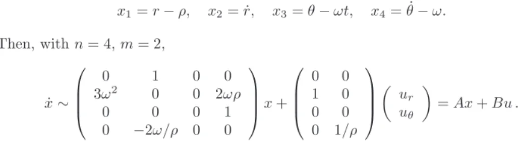
Recall that one reason for taking an interest in linear models is that they tell us about controllability around an equilibrium point. Imagine there is a perturbing force. Take coordinates of perturbation

x1=r−ρ, x2= ˙r, x3=θ−ωt, x4= ˙θ−ω. Then, with n= 4,m= 2, ˙ x_∼     0 1 0 0 3ω2 ₀ ₀ ₂_ωρ 0 0 0 1 0 −2ω/ρ 0 0    x+     0 0 1 0 0 0 0 1/ρ     ur uθ =Ax+Bu .

It is easy to check that M2 =

B AB has rank 4 and that therefore the system is controllable.

But supposeuθ= 0 (tangential thrust fails). Then

B =     0 1 0 0     M4= B AB A2_B _A3_B₌     0 1 0 ₋ω2 1 0 −ω2 ₀ 0 0 −2ω/ρ 0 0 −2ω/ρ 0 2ω3_/ρ    . Since (2ωρ,0,0, ρ2₎_M

4= 0, this is singular and has rank 3. The uncontrollable

compo-nent is the angular momentum, 2ωρδr+ρ2_δ_θ_˙₌_δ₍_r2_θ_˙₎_|

r=ρ,θ=ω˙ .

On the other hand, if ur = 0 then the system is controllable. We can change the

OPTIMIZATION AND CONTROL