Poverty Status and Factors Affecting Household Poverty in Southern Punjab: An Empirical Analysis

(1)

437

Volume and Issues Obtainable at Center for Sustainability Research and Consultancy

Journal of Business and Social Review in Emerging Economies

ISSN: 2519-089X (E): 2519-0326 Volume 6: No. 2, 2020

Journal homepage: www.publishing.globalcsrc.org/jbsee

Poverty Status and Factors Affecting Household Poverty in Southern Punjab: An

Empirical Analysis

1

Salyha Zulfiqar Ali Shah, 2 Imran Sharif Chaudhry, 3 Fatima Farooq 1

Assistant Professor, School of Economics, Bahauddin Zakariya University Multan, Pakistan

salyhazulfiqar@bzu.edu.pk

2

Director, School of Economics, Bahauddin Zakariya University Multan, Pakistan

imran@bzu.edu.pk

3

Assistant Professor, School of Economics, Bahauddin Zakariya University Multan, Pakistan

fatimafarooq@bzu.edu.pk

ARTICLE DETAILS ABSTRACT

History

Revised format: April 2020 Available Online: May 2020

The strategies expected to mitigate poverty tend to identify factors that are closely related to poverty and that could have influenced the policy implications. A household level data was collected to examine the poverty status and factors affecting poverty in Southern Punjab. A logistic regression technique was employed for the present analyses. The findings show that age and education of the household head, own house, spouse participation, remittances, number of earners in the household and physical assets reduces the probability of being poor in Southern Punjab. However, large household size, occupation in the primary sector, high dependency ratio and mental disability are associated with an increased probability of being poor in Southern Punjab. Government should adopt effective policy measures to generate employment and encourage the attainment of education for the poor households for the mitigation of poverty in this region.

Poverty; Southern Punjab; Poverty Alleviation;

Household; Binomial Logit Regression; Poverty Gap; Severe Poverty Gap JEL Classification:

I32, C21, D1, P46

Corresponding author’s email address: salyhazulfiqar@bzu.edu.pk

Recommended citation: Shah, S.Z.A, Chaudhry, I.S & Farooq, F. (2020). Poverty Status and Factors Affecting Household Poverty in Southern Punjab: An Empirical Analysis. Journal of Business and Social Review in Emerging Economies, 6(2), 437-451

DOI: 10.26710/jbsee.v6i2.1151

1. Introduction

All the countries across the world have acknowledged that poverty alleviation has to be of critical importance among the objectives of the economic development. To purse the poverty reduction goal, socio economic, demographic, human development factors should be interlinked for better quality of life and overall economic progress of the poor countries. The present study focuses on Southern Punjab, which comprises of 3 divisions. It is a mainly a developing and backward region of the Punjab. It constitutes mostly on small cities, vast rural and desert areas. Considering the problem of rising poverty in in Southern Punjab, have been focused to analyze the factors Affecting poverty. These divisions have

(2)

438

received very minute prosperity both at the policy and empirical level.

Keeping in view the above discussion, this papers is structured as follows. The section 2, presents the brief over view of existing literature. The section 3 offers data and methodology. The section 4 explain the empirical findings. The section 5 provides the concluding remarks.

2. The Literature Review

Various strands of literature are found on poverty. Moreover, it is generally considered as a plague and extremely serious matter to ponder across the world.

Rodriguez and Smith (1994) found that poverty prevails in those household headed by person having lower education attainment. Poverty can be addressed through developing opportunities, entitlements and capabilities [Sen (1981, 1985)]. Coulombe and Mckay (1996) found that the household living in a rural area, low education, and a high dependency ratio certainly increase the likelihood of being poor. Ravallion (1998) contended the importance of education that let to generate economic growth of developing countries.

Datt and Jolieffe (1999) had scrutinized the major causes of poverty in Egypt for the year 1997. The authors had collected secondary data, using multivariate analysis. The study revealed that education can play a vital role in alleviating poverty. If the adult average years of schooling were improved, this would result in better standard of living of households. An investment in education can raise human capital resources and thus lower the poverty incidence for long term. The policy implication suggested that the better irrigation facilities can be helpful in generating employment opportunities thus reducing the rate of unemployment but also an increase the productivity of agriculture sector in Egypt.

A study by Chaudhry et al. (2006) uncovered rural poverty, employing multivariate regression analysis. Their results interpreted that rural poverty is pervasive and spreading across the rural areas of Pakistan. The poverty correlates were less during the seventies and eighties but again showed a rising trends during nineties. As majority of the rural population heavily linked with agriculture sector directly or indirectly are more vulnerable to poverty incidence. While comparing economic performance with India, the authors concluded that Pakistan have better macroeconomic performance. The major cause of persistent rural poverty was low per capita income, inflation and high unemployment rates of the household.

Rupasingha and Goetz (2007) analyzed the determinants of poverty in United states of America and collected secondary data from household during the year 2000. The authors have divided the study into numerous economical structural, demographic social and political characteristics. The study found that counties in metro regions were less likely to be poor as compare to the counties in the non-metro regions. Counties having high rates of education, more female labor force participation, high employment rates, and higher level of social capital have less poverty during the year 1999. However, counties with high inequal distribution of income, high population of young adults, high ethnic diversity have high level of poverty rate.

Awopeju (2014) discussed the determinants of poverty in Nigeria, during the year 2009-2010 using Foster Greer Thorbecke index (FGT) index to measure the poverty profile. The independent variables were various regional and socioeconomic economic factors. The study showed that 50.4 percent of sample data population was poor at national level and 18.9 percent were poorest. In rural areas, at sub national level, 53.5 percent of population was poor and 32.7 percent of population in the urban areas. The policy implications were that government should play an effective role to enhance the conditions of rural areas and encourage the women empowerment.

The logit regression technique was employed by Edoumiekumo et al. (2014) to discuss the causes of household poverty in geopolitical region of Nigeria. The author collected the data from national living standard survey during the period 2009-10. The study revealed that in rural area the poverty was chronic

(3)

439

issue and effects households in the agricultural sectors. These study had suggested that opportunities, quality education should be provided to the household besides focusing on either its urban or rural. Family size should not be exceeded beyond fived members.

Cheema and Sial (2014) studied the concept of poverty and it determinants in Pakistan. The author collected the secondary data from PSLM data for the households during the year 2010-11, using OLS regression. In this study the dependent variable was log of real expenditure per capita. The results revealed that house hold size, dependency ratio have negative relation with expenditure. Education, education square, urban, shop commercial building, residential building and animal for transportation were positively related to real expenditure per capita. Poverty level was extreme in Balochistan and less in Sindh. The study recommends that free education, reduction in dependency ratio helps in reduction of poverty.

Chen and Wang (2015) examined the poverty status of the household belonging to different 23 cities for Taiwan. The authors had collected secondary data for the year 2006 using hierarchical generalized linear model also known multi levels logistic regression technique. The study concluded that poverty vary across regions. People living in higher income inequality, lower job quality and higher spatial mismatch are more likely to live in poverty. Employment to population ratio, employment in the service and employment in the industry ratio increased than poverty would be reduced.

Biyase and Zwane (2018) studied various indicators Affecting poverty in South Africa. The authors had collected secondary data for the year 2006 using random effect probit estimation technique. The study concluded that education and race of the head of household, dependency ratio, employment status, gender and marital status are essential indicators to mitigate poverty. Households living in urban areas are less prone to poverty, however rural areas are still suffering from poverty in South Africa.

Stems from various studies that majority of people in developing countries are unable to meet their ends and suffering from chronic poverty. The denial of employment opportunities, low infrastructure, lack of education and physical assets and limited access to market have forced poor countries to remain deprived and underdeveloped. This study presents an analysis of indicators that are strongly associated with the poverty status of the household. The next section will present the data and methodology.

3. Data and Methodology

The primary data has been collected through a household survey in Southern Punjab comprising of three divisions during the year 2019. The size of the sample consists of 1068 observations, adopted simple random and stratified sampling.

Measurement of Poverty

FGT is labelled as Foster, Greer and Thorbecke, thoroughly employed in countless theoretical and empirical literature of poverty.

FGTPoverty Index

In 1984, these indices were introduced by, Joel Greer,James Foster, and Erik Thorbecke. It is the most widely used index as it gives more weight on the poverty of the poor individuals. It can be written as:

𝑃_𝛼 (𝑦; 𝑧) = 1 𝑛 ∑ [ 𝑔𝑖 𝑍 ] 𝛼 𝑞 𝑖=1

where z is the poverty line, 𝑔 is the poor, N is the sum of people and yi is the income of each

individual i. The lower the value of α then all the individuals having income below poverty line are more or less same. If the value of α is higher, the greater will be poverty among individuals across the country

(4)

440

It helps to construct and analyze the incidence of poverty. The headcount ratio explains the proportion of the people that is poor. But fails to explain the intensity of the poverty i.e. how much poorer are the poor individuals. 𝐻 = 𝑃0 (𝑦; 𝑧) = 1 𝑛 ∑ [ 𝑍 − 𝑦𝑖 𝑍 ] 0 𝑞 𝑖=1 Poverty Line Calculations

The National Poverty line (2019), measured by employing the national poverty line of 2015-16, amounting to Rs.3250.28, as mentioned in National Poverty Report (2015-16) by Planning Commission of Pakistan. In 2015-16, poverty line was inflated to calculate the poverty line for the year 2019-20, amounting to Rs. 4225.25 per month. According to World Bank (2015), the international estimates for poverty line is 1.90 $. International Poverty line estimated is about $1.90 or less a day in 2015 as mentioned by the world bank and estimated i.e. $1 = Rs. 155.01 for the year 2019, amounting to Rs. 294.5 each day and Rs. 8835.0 each month in Pakistan.

Regression Model

The study used a binomial logistic regression having dependent variable of dichotomous nature. The logistic regression model can be explained through the equation:

Y* = 1 + 2 X 2i +3 X 3i+……….… + k Xki + єi

Y* is the dependent variable representing the Households’ level of poverty and Xs are the various household level socioeconomic and demographic indicators that determine the household level poverty determinants Being a dummy or a dichotomous variable Y can be written in the form of

Yi = 1 , if Yi *

< 0 ; Yi = 0

Thus, logistic equation can be written as







 _ _         _ 



/ / / 1 1 1 / i i i X X X i e e e X F

(5)

441 Table 1: Variables Utilized for Binomial Logit Regression Estimates of Poverty

Variables Description of the Variables Dependent Variable for Binomial Logit Model

Y Poverty = 1 if per capita income is lower than $1.90/day then household is Poor

= 0 if per capita income more than $1.90/day then household is Non Poor

Independent Variables Demographic Variables

HAGE Age of Household head

Complete years of respondent ‘s age HSIZE Household ‘s Size The total person in a household

DR Dependency Ratio Total dependents divided by total household size.

Economic Variables

OCC Occupation of Household Head

= 1 if household head working in primary sector = 0 if household head not working in primary sector

NOEIH Number of Earners The household comprising of total earners LNVOLPA Physical Assets The natural log of value of physical assets own

by the household

OH Own House = 1 if household has own house = 0 if household not own house REM Remittances = 1 if household receive remittances

= 0 if household not receive remittances SP Spouse’s Participation = 1 if the Spouse participate in labor force

= 0 if the Spouse not participate in labor force CRD Access to Credit = 1 if household have an access to credit

= 0 if household have not access to credit

Social variables

MI Mental Disease = 1 if a person in a family is mentally ill = 0 if a person in a family is not mentally ill PD Physical Disability = 1 if any member of household is physically

disable

= 0 if any member of household is not physically disable

HEDU Education of the Household Head

Total years of education

Poverty model

       PHYD MENTD CREDIT SPART REM OH PHYASSETS NOEIH OCC DRATIO HEDU HSIZE HAGE f Y , , , , , , , , , , , ,

The above model in econometric form as:

                         i 13 12 11 10 9 8 7 6 5 4 3 2 1 0 ß ß ß ß ß ß ß ß ß ß ß ß ß ß ß PHYD MENTD CREDIT SPART REM OH PHYASSETS NOEIH OCC DRATIO HEDU HSIZE HAGE f Y

(6)

442

4. Empirical Findings

This section begins by analyzing and examining the factors Affecting poverty of the households in Southern Punjab in the Table 4. With the increase in the household head age by one year, the probability of poverty reduces by 0.9 percent [Rodriguez, 2002; Gang et al.,2004; Arif and Farooq, 2014]. If the size of household increases by one person, there is 8.6 percent probability of increasing poverty [Arif and Bilquess,2007; Litchfield and McGregor, 2009; Arif and Farooq, 2014]. If the household head is one year more educated, the probability of poverty declines by 5.5 percent [Bundervoet (2006), Zuluaga (2007)]. There is 17.8 percent likelihood of increasing poverty level, if the occupation of the respondent is associated with the primary sector [Agenor and Montiel, 1996; Carruth and Oswald1981; Kar and Marjit, 2001]. Due to the increase in dependency ratio there is 12.3 percent probability of increasing poverty of the household [Dreze and Srinivasan, 1997; Hashmi et al., 2008]

With the increase in mental disability of any person in the household, the probability of poverty increases by 66.2 percent [Yeo and Moore(2003), Kessler et al., (2005) and Hoogeveen, 2005)].Moreover, its 7.3 percent probability of increasing poverty if any member of the household is suffering from physical disability [Sikander and Ahmed (2008), Rahman (2013), Arif and Farooq (2014)]. The 42.9 percent probability of declining poverty if the household have their own house [Arif and Bilquees (2007), Ahmad and Sadaqat (2016)]. If there is an increase in spouse’s participation, almost 28.9 percent probability of reducing poverty of the household. These results support the studies by Mincer (1962), Kozel and Alderman (1990). With the increase in remittances received by the household, the probability of poverty reduces, by 32.1 percent. These results support the studies by Inoue (2018) and Vacaflores (2018). The probability of poverty declines by 7.5 percent, if the household have the access to credit or availability of credit facilities. [Pitt and Khandker (1998), Remenyi and Benjamin (2000), Coleman (2002), Khandker (2003) and Quach et al., (2005)].

The probability of poverty decreases by 6.6 percent if the number of earners in the household increases by one person [Sikander and Ahmed (2008), Ahmed and Sadaqat (2016)]. There is 3.3 percent probability of reducing poverty, with the increase in the value of the physical assets of the household [Ravallion & Jalan, (1998), Sackey (2005), Bigsten and Shimeles (2008)].

Table 2: Descriptive Analysis of Poverty in Southern Punjab.

Variables _Mean _{Standard Deviation}

Poverty 0.40 0.49

Mental Disability 0.09 0.29

Value Of Physical Assets 4834496 11281889

Number Of Earners in the Household 2.04 1.08

Occupation 0.57 0.50

Own House 0.90 0.30

Remittances 0.12 0.32

Spouse's Participation 0.16 0.37

Household Size 6.34 2.55

Education of Household Head 8.29 5.56

Age of the Household Head 48.18 12.76

Dependency Ratio 0.75 0.73

Access to Credit 0.12 0.33

Physical Disability 0.11 0.31

(7)

443 Table 3: Correlation Analysis of Poverty and its Correlates in Southern Punjab

Probability Y HAGE HSIZE HEDU OCC DR MI PD OH SP REM CRD NOEIH PHYASSET Y 1.000 HAGE -0.111 (0.000) 1.000 HSIZE 0.237 (0.000) 0.322 (0.000) 1.000 HEDU -0.578 (0.000) -0.056 (0.066 -0.146 (0.000) 1.000 OCC 0.470 (0.000) -0.020 (0.514) 0.089 (0.004) -0.600 (0.000) 1.000 DR 0.329 (0.000) -0.135 (0.000) 0.195 (0.000) -0.184 (0.000) 0.181 (0.000) 1.000 MI 0.334 (0.000) -0.058 (0.059) 0.066 (0.031) -0.254 (0.000) 0.252 (0.000) 0.068 (0.026) 1.000 PD 0.153 (0.000) 0.153 (0.000) 0.104 (0.001) -0.146 (0.000) 0.150 (0.000) 0.043 (0.157) 0.048 (0.116) 1.000 OH -0.284 (0.000) 0.146 (0.000) 0.020 (0.513) 0.183 (0.000) -0.131 (0.000) 0.033 (0.284) -0.146 (0.000) -0.084 (0.006) 1.000 SP -0.237 (0.000) 0.144 (0.000) 0.085 (0.005) 0.127 (0.000) -0.146 (0.000) -0.199 (0.000) -0.060 (0.049) -0.009 (0.768) 0.081 (0.008) 1.000 REM -0.216 (0.000) 0.020 (0.512) 0.010 (0.740) 0.133 (0.000) -0.118 (0.000) -0.148 (0.000) -0.063 (0.040) 0.005 (0.871) 0.121 (0.000) 0.194 (0.000) 1.000 CRD -0.008 (0.790) -0.006 (0.840) 0.020 (0.508) -0.003 (0.923) 0.066 (0.031) 0.018 (0.560) 0.031 (0.309) 0.079 (0.010) 0.012 (0.705) 0.010 (0.755) 0.050 (0.100) 1.000 NOEIH -0.182 (0.000) 0.356 (0.000) 0.469 (0.000) 0.089 (0.004) -0.090 (0.003) -0.391 (0.000) -0.095 (0.002) 0.020 (0.523) 0.144 (0.000) 0.369 (0.000) 0.227 (0.000) 0.072 (0.018) 1.000 PHYASSET -0.059 (0.054) 0.035 (0.259) -0.030 (0.323) 0.016 (0.597) -0.076 (0.013) 0.032 (0.293) -0.039 (0.207) 0.005 (0.860) 0.041 (0.180) 0.060 (0.051) 0.073 (0.017) -0.038 (0.217) 0.000 (1.000) 1.000

Source: Survey data, 2019; probabilities in brackets.

Table 4: Results of the Factors Affecting Poverty in Southern Punjab Dependent Variable: Poverty ( if Poverty = 1 , Otherwise = 0) Variable Marginal Effects Coefficients Standard Errors z-Statistic Probability C --- 4.123 0.826 4.992 0.000

Household Head Age -0.009 -0.037 0.008 -4.525 0.000

Household Size 0.086 0.370 0.056 6.566 0.000 Education of Household Head -0.055 -0.231 0.023 -10.176 0.000 Occupation 0.178 0.745 0.228 3.269 0.001 Dependency Ratio 0.123 0.514 0.159 3.229 0.001 Mental Disability 0.662 2.765 0.564 4.898 0.000 Physical Disability 0.073 0.308 0.317 0.972 0.331 Own House -0.429 -1.790 0.356 -5.035 0.000 Spouse 's Participation -0.289 -1.209 0.329 -3.672 0.000 Remittances -0.321 -1.341 0.392 -3.420 0.001 Access to Credit -0.075 -0.314 0.292 -1.075 0.282 Number of earners in Household -0.066 -0.277 0.129 -2.143 0.032

Value of Physical Assets -0.033 -0.136 0.048 -2.847 0.004

McFadden R-squared 0.498 Mean dependent var 0.397

LR statistic 715.128 Prob. (LR statistic) 0.000

Source: Survey data, 2019

(8)

444

Division. If there is an incline in the age of the household head by one year, the probability of poverty reduces by 1.1 percent. [Datt and Jolliffe (1999)]. If the size of household increases by one person, there is 9.12 percent probability of increasing poverty, noted significant values at 1 percent level [Sikander and Ahmed (2008)]. If the household heads are one year more educated, the probability of poverty declines by 5.7 percent [Sen (1981), Arif and Farooq (2014), Ahmed and Sadaqat, (2016)]. There is 18.6 percent probability of increasing poverty if the occupation of the household head is attached with the primary sector [Mukherjee and Benson, 1998)].

An increase of dependency ratio of the family, it leads to 13.3 percent probability of increasing poverty of the household [Jamal (2005)]. With an increase of mental illness of any member in the household, the probability of poverty increases by 71.6 percent. There is 5.11 percent probability of increasing poverty of the household, if any member of the household is suffering from physical disability [Neilson et al., (2008)]. The econometric results of the own house of the household, the 43.25 percent probability of declining poverty if the household have their own house. There is 32.17 percent probability of lesser poverty of the household, if spouse’s participation increases in economic activities [Mincer (1962), With the increase in remittances by one unit received by the household, the probability of poverty reduces by 39.9 percent [Ranathunga et al., (2010]. With the increase in the access to credit or availability of credit facilities by the household, the probability of poverty declines by 5.8 percent. The probability of poverty decreases by 5.18 percent if the number of earners in the household increases by one person. There is 0.5 percent probability of reducing poverty, with the increase in the value of the physical assets of the household [Hashmi et al., (2008) and Neilson at al., (2008)].

Table 5: Results of the Factors Affecting Poverty in Multan Division

Dependent Variable : Poverty ( if Poverty = 1 , Otherwise = 0) Variable Marginal Effects Coefficients Standard Errors z-Statistic Probability C --- 2.463 1.489 1.654 0.098

Table 6 presents the binomial logistic regression results of the factors affecting poverty in Bahawalpur division. With an increase in household head age by one year, the probability of poverty reduces by 1.1 percent. If the size of household increases by one person, there is 7.5 percent probability of increasing poverty [Gang et al., (2008) and Hashmi et al., (2008)]. If the household head is one year more educated,

(9)

445

the probability of poverty declines by 6.1 percent. [Datt and Jolliffe (1999). There is 12.2 percent probability of increasing poverty if the occupation of the respondent is associated with the primary sector. Due to the increase in dependency ratio there is 16.2 percent probability of increasing poverty of the household. [Hashmi et al., (2008)]. With the presence of mental disability of any member in the household, the probability of poverty increases by 82.6 percent. There is 2.7 percent probability of increasing poverty if any member of the household is suffering from physical disability. There is 32.4 percent probability of declining poverty if the household have their own house. If there is spouse’s participation in economic activities, there is 41.8 percent probability of declining poverty of the household. With the increase in remittances received by the household, the probability of poverty reduces by 21.5 percent. The probability of poverty declines by 20.4 percent, if the household have the access to credit or availability of credit facilities. The probability of poverty decreases by 3.3 percent if the number of earners in the household increases by one person. There is 8.1 percent probability of reducing poverty, with the increase in the value of the physical assets own by the household.

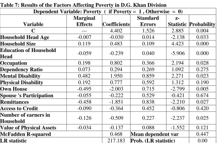
Table 7 presents the binomial logistic regression results of the factors affecting poverty in D.G. Khan division. With the increase in the household head age by one year, the probability of poverty reduces by 0.7 percent. If the size of household rise by one member, there is 11.9 percent probability of increasing poverty. If the household head is one year more educated, the probability of poverty declines by 5.9 percent [Arif and Bilquess (2007)]. There is, 19.8 percent probability of increasing poverty if the occupation of the respondent is associated with the primary sector [Kar and Marjit, (2001)]. Due to the increase in dependency ratio, lead to 7.3 percent probability of increasing poverty of the household. [Dreze and Srinivasan (1997)]. With the increase in mental disability of any member in the household, the probability of poverty increases by 48.2 percent. There is 19.2 percent probability of increasing poverty, if any member of the household is suffering from physical disability. This shows that its 49.5 percent probability of declining poverty if the household have their own house. If there is spouse’s participation in economic activities, there is 5.5 percent probability of lowering poverty of the household. An increase in remittances received by the household, the probability of poverty reduces by 45.8 percent [Arif and Bilquees (2007); Hashmi et al., (2008)]. The probability of poverty declines by 9 percent, if the household have the access to credit or availability of credit facilities. However, the probability of poverty decreases by 12.6 percent if the number of earners in the household increases by one person. There is 3.4 percent probability of reducing poverty, with the increase in the value of the physical assets of the household [Ahmed and Sadaqat (2016)].

(10)

446

Table 6: Results of the Factors Affecting Poverty in Bahawalpur Division Dependent Variable: Poverty (if Poverty =1, Otherwise = 0) Variable Marginal Effects Coefficients Standard Errors z-Statistic Probability C --- 7.168 1.644 4.359 0.000

Table 7: Results of the Factors Affecting Poverty in D.G. Khan Division Dependent Variable: Poverty ( if Poverty = 1 , Otherwise = 0) Variable Marginal Effects Coefficients Standard Errors z-Statistic Probability C --- 4.402 1.526 2.885 0.004

(11)

447

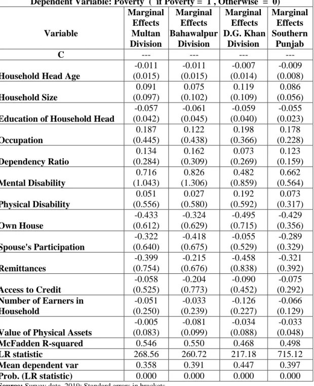
Table 8 presents the comparative analysis of the econometric results of the factors affecting poverty in Southern Punjab and its division,

Table 8: Comparative Analysis of Factors Affecting Poverty in Southern Punjab and its Division

Dependent Variable: Poverty ( if Poverty = 1 , Otherwise = 0)

Variable Marginal Effects Multan Division Marginal Effects Bahawalpur Division Marginal Effects D.G. Khan Division Marginal Effects Southern Punjab C --- --- --- ---

Household Head Age

-0.011 (0.015) -0.011 (0.015) -0.007 (0.014) -0.009 (0.008) Household Size 0.091 (0.097) 0.075 (0.102) 0.119 (0.109) 0.086 (0.056)

Education of Household Head

-0.057 (0.042) -0.061 (0.045) -0.059 (0.040) -0.055 (0.023) Occupation 0.187 (0.445) 0.122 (0.438) 0.198 (0.366) 0.178 (0.228) Dependency Ratio 0.134 (0.284) 0.162 (0.309) 0.073 (0.269) 0.123 (0.159) Mental Disability 0.716 (1.043) 0.826 (1.306) 0.482 (0.859) 0.662 (0.564) Physical Disability 0.051 (0.556) 0.027 (0.580) 0.192 (0.592) 0.073 (0.317) Own House -0.433 (0.612) -0.324 (0.629) -0.495 (0.715) -0.429 (0.356) Spouse's Participation -0.322 (0.640) -0.418 (0.675) -0.055 (0.529) -0.289 (0.329) Remittances -0.399 (0.754) -0.215 (0.676) -0.458 (0.838) -0.321 (0.392) Access to Credit -0.058 (0.525) -0.204 (0.773) -0.090 (0.452) -0.075 (0.292) Number of Earners in Household -0.051 (0.250) -0.033 (0.239) -0.126 (0.227) -0.066 (0.129)

Value of Physical Assets

-0.005 (0.083) -0.081 (0.099) -0.034 (0.088) -0.033 (0.048) McFadden R-squared 0.546 0.550 0.468 0.498 LR statistic 268.56 260.72 217.18 715.12

Mean dependent var 0.358 0.391 0.447 0.397

Prob. (LR statistic) 0.000 0.000 0.000 0.000

(12)

448

Table 9: Poverty Status at National Poverty line Regions Location Poor Non

Poor Total Households Poverty Incidence (%) Poverty Gap (%) Squared Poverty Gap (%) Southern Punjab Total 299 769 1068 27.99 10.55 5.06 Rural 272 552 824 33.00 12.78 6.20 Urban 27 217 244 11.06 3.03 1.20 Multan Division Total 101 276 377 26.79 10.14 4.84 Rural 90 193 283 31.80 12.44 6.01 Urban 11 83 94 11.70 3.21 1.29 Bahawalpur Division Total 98 255 353 27.76 10.61 5.03 Rural 87 177 264 32.95 12.8 6.16 Urban 11 78 89 14.10 4.01 1.29 D.G. Khan Division Total 100 238 338 29.58 10.95 5.33 Rural 95 182 277 34.29 13.07 6.43 Urban 5 56 61 8.19 1.33 0.31

Table10: Poverty Status at International Poverty line Regions Location Poor

Non-Poor Total Households Poverty Incidence (%) Poverty Gap (%) Squared Poverty Gap (%) Southern Punjab Total 425 643 1068 39.79 22.93 15.31 Rural 348 476 824 42.23 26.30 18.04 Urban 77 167 244 31.15 11.52 6.11 Multan Division Total 135 242 377 35.80 21.87 14.72 Rural 109 174 283 38.51 25.53 17.60 Urban 26 68 94 27.65 10.83 6.05 Bahawalpur Division Total 138 215 353 39.90 22.86 15.32 Rural 110 154 264 41.16 26.40 18.12 Urban 28 61 89 31.46 12.34 6.99 D.G. Khan Division Total 151 187 338 44.67 24.18 15.97 Rural 129 148 277 46.57 27.00 18.41 Urban 22 39 61 36.06 11.38 4.91

5. Concluding Remarks

This paper explains the poverty status and factors Affecting poverty in Southern Punjab, consisting of three divisions which are Multan, Bahawalpur and D.G. Khan division. The study consisting of 1068 observations, using Binomial Logit regression is used for empirical analysis. The poverty status is measured with the help of head count poverty ratio and after comparative analysis, hence concluded that D.G Khan division is the poorest division (29.58%) based on national and (44.67 %) at international poverty line in Southern Punjab, Pakistan.

(13)

449

The finding concludes that house hold size, occupation of the household head in the primary sector, dependency ratio, physical disability and mental disability shows a positive correlation with poverty of the household in Southern Punjab. However, the education of the household head, remittances, spouse's participation, number of earners in the household, access to credit, own house and value of physical assets shows a negative correlation with poverty in Southern Punjab.

The analysis discussed above assist the policy makers to clearly identify the factors for poverty alleviation in Southern Punjab. Poverty can only be reduced by generating employment opportunities for the people in the country. Government should establish different scientific, technical training, and skill development schools and institutes for both male and female workers to increase their productivity so they can collectively contribute in raising the real GDP of the poor countries like Pakistan.

Moreover, provision of educational facilities are crucial equally for males and females in the society. As drawn from the conclusion that spouse participation mitigates the poverty, therefore suggested that educational attainment for females are likewise mandatory and essential. Government should develop strategies to encourage and support female participation in economic activates so they not only become financially strong but also contribute in the growth and development of the poor countries like Pakistan.

References

Ahmad, N., & Sadaqat, M. (2016). Social Capital Household Welfare and Poverty: Evidence from Pakistan. The Pakistan Development Review, 467-482.

Agenor, P & P. Montiel, 1996, Development Macroeconomics, Princeton, NJ: Princeton University Press Arif, G. M., & Bilquees, F. (2007). Chronic and Transitory Poverty in Pakistan: Evidence from A

Longitudinal Household Survey. The Pakistan Development Review, 111-127

Arif, G. M., & Farooq, S. (2014). Rural Poverty Dynamics in Pakistan: Evidence from Three Waves of the Panel Survey. The Pakistan Development Review, 53(2), 71-98.

Awopeju, S, O. (2014 June 23-26). Determinants of Poverty Depth Among Households in Rural Urban Nigeria. Paper Presented at The 14th EADI General Conference, Bonn, Germany.

Bigsten, A., & Shimeles, A. (2008). Poverty Transition and Persistence in Ethiopia: 1994–2004. World Development, 36(9), 1559-1584.

Biyase, M., & Zwane, T. (2018). An Empirical Analysis of the Determinants of Poverty and Household Welfare in South Africa. The Journal of Developing Areas, 52(1), 115-130.

Bundervoet, T. (2006) Estimating Poverty in Burundi. Households in Conflict Network (Hicn). (Working Paper No. 20.

Carruth, A. A., & Oswald, A. J. (1981). The Determination of Union and Non-Union Wage Rates. European Economic Review, 16(2), 285-302

Chaudhry, I.S. (2007), "Impact of Gender Inequality in Education On Economic Growth: An Empirical Evidence from Pakistan", The Pakistan Horizon Vol. 60, No. 4,

Cheema, A. R., & Sial, M. H. (2014). Poverty and Its Determinants in Pakistan: Evidence from Pslm 2010-11. Journal of Poverty, Investment and Development, 5, 1-16.ATE

Chen, K. M., & Wang, T. M. (2015). Determinants of Poverty Status in Taiwan: A Multilevel Approach. Social Indicators Research, 123(2), 371-389.

Coleman, B. E. (2002), "Microfinance in Northeast Thailand: Who Benefits and How Much?" Asian Development Bank - Economics and Research Department Working Paper 9.

Coulombe, H. And A. Mckay (1996) Modeling Determinants of Poverty in Mauritania. World Development 24:6, 1015–31.

Datt, G., & Jolliffe, D. (1999). Determinants of Poverty in Egypt, 1997 (No. 75). International Food Policy Research Institute (IFPRI).

Dreze, J., & Srinivasan, P. V. (1997). Widowhood and Poverty in Rural India: Some Inferences from Household Survey Data. Journal of Development Economics, 54(2), 217-234.

(14)

450

Edoumiekumo, S, G., Karimo, T, M., & Tombofav, S, S. (2014). Determinants of Households’ Income Poverty in The South-South Geopolitical Zone of Nigeria. Journal of Studies in Social Sciences, 9(1), 101-115.

Gang, I. N., Sen, K., & Yun, M. S. (2008). Poverty in Rural India: Caste and Tribe. Review of Income and Wealth, 54(1), 50-70.

Hashmi, A, A., & Sial, M, H. (2008). Trends and Determinants of Rural Poverty: A Logistic Regression Analysis of Selected Districts Of Punjab. The Pakistan Development Review, 47(4), 909–923.

Hoogeveen, J. G. (2005). Measuring Welfare for Small but Vulnerable Groups: Poverty and Disability in Uganda. Journal of African Economies, 14(4), 603-631.

Inoue, T. (2018). Financial Development, Remittances, And Poverty Reduction: Empirical Evidence from A Macroeconomic Viewpoint. Journal of Economics and Business, 96, 59-68.

Jamal, H. (2005). In Search of Poverty Predictors: The Case of Urban and Rural Pakistan. The Pakistan Development Review, 37-55

Kar, S & S, Marjit. (2001). Informal Sector in General Equilibrium: Welfare Effects of Trade Policy Reforms, International Review of Economics and Finance, 10, 289-300.

Kessler, R. C., Chiu, W. T., Demler, O., & Walters, E. E. (2005). Prevalence, Severity, And Comorbidity of 12-Month DSM-IV Disorders in The National Comorbidity Survey Replication. Archives of General Psychiatry, 62(6), 617-627.

Khandker, S. R. (2003), "Microfinance and Poverty: Evidence Using Panel Data from Bangladesh", World Bank Policy Research Working Paper 2945.

Kozel, V., And H. Alderman (1990), “Factors Determining Work Participation and Labour Supply Decisions in Pakistan’s Urban Area”, The Pakistan Development Review, 29:1, 1-18.

Litchfield, J. And Mcgregor, T. (2008). Poverty in Kagera, Tanzania: Characteristics, Causes and Constraints. PRUS Working Paper No.42. University of Sussex, Brighton. United Kingdom

Mincer, J. (1962), “Labour Force Participation of Married Women: A Study of Labour Supply. In H. G. Lowis (Ed.) Aspects of Labour Economics”, Princeton, N. J.: Princeton University Press. 63-97. Mukherjee, S., & Benson, T. (2003). The Determinants of Poverty in Malawi, 1998. World

Development, 31(2), 339-358.

Neilson, C., Contreras, D., Cooper, R., & Hermann, J. (2008). The Dynamics of Poverty in Chile. Journal of Latin American Studies, 40(2), 251-273

Partridge, M. D., & Rickman, D. S. (2007). Persistent Rural Poverty: Is It Simply Remoteness and Scale? Review of Agricultural Economics, 29(3), 430-436.Ben

Pitt, M., And S., Khandker (1998), "The Impact of Group-Based Credit Programs On Poor Households in Bangladesh: Does The Gender of Participant’s Matter?", Journal of Political Economy, Vol. 106, No. 5, Pp. 958-995.

Quach, M., Mullineux, A., & Murinde, V. (2005). Access to Credit and Household Poverty Reduction in Rural Vietnam: A Cross-Sectional Study. The Birmingham Business School, The University of Birmingham Edgbaston, 1-40.

Rahman, M. A. (2013). Household Characteristics and Poverty: A Logistic Regression Analysis. The Journal of Developing Areas, 303-317.

Ranathunga, S., & Gibson, J. (2014). Determinants of Household Poverty in The Rural Sector in Sri Lanka: 1990-2010. Economics, 3(3), 43-49.

Ravallion, M. (1998). Poverty Lines in Theory and Practice. The World Bank.

Ravallion, M., & Jalan, J. (1998). Determinants of Transient and Chronic Poverty: Evidence from Rural China. The World Bank

Remenyi, J., And Q., Benjamin. (2000), Microfinance and Poverty Alleviation: Case Studies from Asia and The Pacific. Pp. 131-134 And 253-263. London And New York: Printer, Continuum Press. Rodriguez, A. G., & Smith, S. M. (1994). A Comparison of Determinants of Urban, Rural and Farm

Poverty in Costa Rica. World Development, 22(3), 381-397.

Rupasingha, A., & Goetz, S, J. (2007). Social and Political Forces as Determinants of Poverty: A Spatial Analysis. The Journal of Socio-Economics, 36, 650–671.

(15)

451

Technique. African Development Review, 17(1), 41-69.

Sen, A.K. (1981), Poverty and Famines, Oxford University Press, Oxford.

Sen, A.K. (1985). A Sociological Approach to The Measurement of Poverty: A Reply to Professor Peter Townsend. Oxford Economic Papers, 37(4), 669-676.

Sikander, M. U., & Ahmed, M. (2008). Household Determinants of Poverty in Punjab: A Logistic Regression Analysis of MICS (2003-04) Data Set. In 8th Global Conference On Business & Economics (Pp. 1-41).

Vacaflores, D. E. (2018). Are Remittances Helping Lower Poverty and Inequality Levels in Latin America? The Quarterly Review of Economics and Finance, 68, 254-265.

World Bank (2015). Global Poverty Line Update.

Https://Www.Worldbank.Org/En/Topic/Poverty/Brief/Global-Poverty-Line-Faq

Yeo, R., & Moore, K. (2003). Including Disabled People in Poverty Reduction Work: “Nothing About Us, Without Us”. World Development, 31(3), 571-590.

Zuluaga, B. (2007) Different Channels of Impact of Education On Poverty: An Analysis for Colombia. Discussion Paper, Available at SSRN 958684