STATISTICAL METHODS FOR PATIENT
CHEMOSENSITIVITY PREDICTION BASED ON
IN VITRO DOSE-RESPONSE DATA AND A
MODIFIED EXPECTATION-MAXIMIZATION (EM)
ALGORITHM FOR REGRESSION ANALYSIS OF
DATA WITH NON-IGNORABLE NON-RESPONSE
by
Yang Zhang
BS, Nanjing University, China, 2006
MS, Northeastern University, 2008
Submitted to the Graduate Faculty of
the Graduate School of Public Health in partial fulfillment
of the requirements for the degree of
Doctor of Philosophy
University of Pittsburgh
2013
UNIVERSITY OF PITTSBURGH GRADUATE SCHOOL OF PUBLIC HEALTH
This dissertation was presented by
Yang Zhang
It was defended on November 22, 2013
and approved by
Gong Tang, PhD, Associate Professor
Department of Biostatistics, Graduate School of Public Health, University of Pittsburgh Joseph P. Costantino, DrPH, Professor
Department of Biostatistics, Graduate School of Public Health, University of Pittsburgh Joyce Chang, PhD, Associate Professor
Division of General Internal Medicine, School of Medicine, University of Pittsburgh Priya Rastogi, MD, Associate Professor
Division of Hematology/Oncology, School of Medicine, University of Pittsburgh Shuguang Huang, PhD, Associate Vice President
Deptpartment of Statistics, Precision Therapeutics Inc., Pittsburgh, PA Dissertation Director: Gong Tang, PhD, Associate Professor
Copyright c by Yang Zhang 2013
STATISTICAL METHODS FOR PATIENT CHEMOSENSITIVITY PREDICTION BASED ON IN VITRO DOSE-RESPONSE DATA AND A MODIFIED EXPECTATION-MAXIMIZATION (EM) ALGORITHM FOR
REGRESSION ANALYSIS OF DATA WITH NON-IGNORABLE NON-RESPONSE
Yang Zhang, PhD University of Pittsburgh, 2013
ABSTRACT
The first part of this dissertation concerns statistical analysis of in vitro assay data derived from tumor cells. An in vitro assay, ChemoFxR, has been developed to predict
patient’s clinical chemosensitivity. We explore statistical methods that can more efficient-ly use the assay data and improve the prediction of clinical outcome. In typical anaefficient-lysis of assay dose-response data, summary statistics such as the area under the dose-response curve, and concentration at half inhibition (IC50) are estimated from the assay data, then these statistics are dichotomized to predict the clinical outcome as sensitive or resistant. Considering the rigidness of the traditional models for dose-response curve fitting and the information loss in use of cell counts in the control wells, here we propose a mixture of expo-nential functions for fitting the dose-response curve and a branching process-based method to summarize the control well data. Simulation studies and analysis of clinical trial data show that the proposed method improves the prediction performance over some traditional methods. The second part concerns statistical analysis of regression data with nonresponses. Missing data are prevalent in clinical trials and public health studies. The often unknown mechanism for the missing data process may actually be associated with the underlying
values. Standard statistical methods, including likelihood-based methods and weighted es-timating equations, require a model for the missing-data mechanism and incorporate it in the estimation and inference. Misspecification of the missing-data model often causes bi-ased estimates and wrongful conclusions. The expectation-maximization (EM) algorithm is an iterative algorithm that is often used to find the maximum likelihood estimate for the likelihood-based methods. In the E-steps, given a current estimate and the missing-data mechanism, the conditional expectations of the sufficient statistics are calculated. Under the premise that the current estimate is consistent, we find that those conditional expectations could be approximated from the empirical data without the need for assuming or modeling the missing-data mechanism. Subsequently, we propose a modified EM algorithm regardless of the potential missing-data mechanism. Simulation studies show that the parameter es-timates have negligible bias and are more efficient than the initial eses-timates obtained from external data.
Keywords: Dose-response curve; Curve fitting; Branching process; Analysis of missing data; Non-ignorable nonresponse; EM algorithm.
TABLE OF CONTENTS
PREFACE . . . xi
1.0 INTRODUCTION . . . 1
1.1 Classification of assay dose-response data . . . 1
1.2 Statistical analysis of missing data . . . 3
2.0 STATISTICAL METHODS FOR PATIENT CHEMOSENSITIVITY PREDICTION BASED ON IN VITRO DOSE-RESPONSE DATA . . 5
2.1 Overview of analysis of assay dose-response data . . . 5
2.1.1 Cancer biomarkers and ChemoFxR assay . . . . 5
2.1.2 Review of metrics for quantifying dose-response assay . . . 7
2.2 The Proposed methods for classification based on dose-response data . . . . 13
2.2.1 Five-parameter mixture of exponential function (5ME) method . . . . 13
2.2.2 Branching process using dose-0 cell counts data . . . 16
2.3 Simulation studies . . . 20
2.3.1 Comparing 5ME, IC50, and AUC using simulated cell counts data . . 20
2.3.2 Comparing 5ME, IC50, and AUC using simulated dose-response curves 22 2.4 Application to clinical trial data . . . 25
2.4.1 Analysis of B40 trial data . . . 25
2.4.2 Analysis of PTI-206 ChemoFxR assay data . . . . 30
2.5 Discussions . . . 33
3.0 A MODIFIED EM ALGORITHM FOR REGRESSION ANALYSIS OF DATA WITH NON-IGNORABLE NON-RESPONSE . . . 35
3.1.1 Missing data in practice . . . 35
3.1.2 Statistical methods for analysis of missing data . . . 37
3.2 EM algorithm for regression analysis of data with non-responses when the missing-data mechanism is modeled. . . 43
3.3 A modified EM algorithm for regression analysis of data with non-responses 45 3.3.1 EM algorithm for regression analysis of data with non-responses when missing-data mechanism is known . . . 46
3.3.2 An modified EM algorithm . . . 47
3.3.3 Implementation of proposed methods in simple linear regression . . . 49
3.3.4 Improvement of modified EM algorithm by involving external data . . 51
3.3.5 The modified EM algorithm under discrete covariates . . . 52
3.3.6 Smoothing methods and its implementation in the modified EM algorithm 52 3.4 Simulation studies . . . 54
3.4.1 Simulation setup . . . 54
3.4.2 Simulation results . . . 56
3.5 Analysis of qualify-of-life data from a cancer clinical trial . . . 59
3.6 Summary and discussion . . . 60
LIST OF TABLES
1 Comparison of 5ME, IC50 and AUC based on simulated cell counts. . . 22
2 Comparing 5ME, IC50 and AUC using simulated dose-response data . . . 23
3 Comparison of methods using B40 ChemoFx assay data . . . 29
4 Comparison of methods by AUROC based on PTI-206 assay data. . . 31
5 Simulation results when the predictor X ∼BIN(5,0.3) . . . 57
6 Simulation results when the predictor X ∼N(0,1) . . . 58
LIST OF FIGURES
1 Layout of a typical 384 (16×24) - well plate in the ChemoFxR Assay . . . . 7 2 Dose response curves (DRCs) of the breast specimens treated with sunitinib.
Responsive (R) specimens are denoted with a solid black line 3/39 (7.6%), intermediate responsive (IR) specimens are delineated with a dashed black line 8/39 (20.5%) and non-responsive (NR) specimens are indicated by a gray line 28/39 (71.7%) . . . 8
3 Definition of IC50, relative IC50 and AUC on a DRC. . . 10
4 Four-parameter logistic function (4PL). 4PL with (β1, β2, β2, β4) = (1,0.2,1,5) is corresponding to the red curve, 4PL with (β1, β2, β2, β4) = (1,0.2,3,5) is
corresponding to the green curve. . . 12
5 Mean of DRCs of the breast specimens treated with doxorubicin (A). Speci-mens from pathological complete response (pCR) groups are corresponding to the red line, specimens from non-pCR groups are corresponding to the black line. . . 14
6 Five-parameter mixture of exponential function (5ME). 5ME with (a, b, c, d, ρ) = (0.01,0.4,0.05,0.5,0.8) is corresponding to the red curve, 5ME with (a, b, c, d, ρ) = (0.01,0.4,0.05,0.5,0.2) is corresponding to the green curve. . . 15
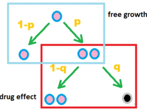
7 Branching Process: free growth and drug effect . . . 17
8 Mean DRCs of simulated cell counts data. . . 21
9 Mean of Simulated DRC following seven-parameter mixture of a 4PL function and an exponential function (7MEL) functions. . . 24
11 Sample dose-response curves in assay with drug A or T, grouped by pCR of
patients in NSABP B-40 Arm 1A. . . 28
12 Mean dose-response curves(DRC’s) in assay with drug A or T, grouped by pCR of patients in NSABP B-40 Arm 1A. . . 29
13 Comparison of methods by ROC analysis using PTI-206 assay data . . . 32
14 Plots of simulated data (x,y) in different scenarios. . . 55
PREFACE
I would like to offer my sincere gratitude to Dr. Gong Tang, my advisor. In the past t-wo and half years, he has supported me in research with his knowledge, enthusiasm, and commitment. Without his guidance and inspiration, the modified EM algorithm would not have been possible. Besides research support, he has also shared with me his wisdom and experience in life.
I would like to thank Dr. Shuguang Huang, my supervisor during my internship at Pre-cision Therapeutics Inc. He has given me important support and advice in the study of dose-response-curve classification (Part I). It is the career experience he has shared with me that has guided me to industry.
I also thank Dr. Joyce Chang, my previous graduate student researcher (GSR) super-visor and Dr. Joseph Costantino, my current GSR supersuper-visor. They have both provided invaluable guidance and have given me the flexibility to balance between my research and GSR work.
Last but not the least, I thank my parents, for giving me the opportunity of life, and their unconditional and consistent love.
1.0 INTRODUCTION
1.1 CLASSIFICATION OF ASSAY DOSE-RESPONSE DATA
ChemoFxR assay is an experimental tool that uses a patient’s tumor chemoresponsein vitro
to predict the patient’s clinical response. This technology has been used in clinical practice for some time to help physicians in treatment decision [Ochs et al., 2005.].
In vitro assays, e.g. ChemoFx, are usually conducted in a dose-response fashion, with tumor cells exposed to a series of a monotonically increasing dosages of the chemotherapeu-tic agent of interest[Brower et al., 2008]. The goal is to use the in vitro assay results to predict patients’ clinical outcome such as clinical/pathological response, disease progression or survival. Typically, the analysis of assay data is involved with two stages: first, the dose-response data is reduced to some summary statistics, such as area under the dose-dose-response curve (AUC), the drug concentration that achieves a target effect (e.g. IC50); these sum-mary statistics are then used to predict the clinical outcome using some statistical methods (e.g., logistic regression model or Cox model).
The relationship between the in vitro and in vivo systems is usually complex. Traditional methods such as AUC (usually based on non-parametric approach, using trapezoidal rule) and IC50 (usually based on 4-parameter logistic regression (4PL)) sometimes can not well differentiate sensitive and resistant curves. Four parameter logistic model (4PL) -derived IC50 shows some relative advantage comparing with the summation of the last three re-sponses on the dose-response curve [Huang and Pang, 2008], but the 4PL parametric curve fitting requires the compliance of the data. For instance, the observed data have to show
a sigmoidal shape as well as the lower and higher plateaus. In reality, though, the data do not always satisfy these requirements. Therefore, we propose a five-parameter mixture of exponential functional form (5ME) which is more flexible in modeling dose-response curves. Similar to the 4PL method, the fitted parameters of 5ME have explicit biological meanings and can be used as predictors in the second stage of patient classification.
Typically, the dose-response curve fitting (e.g. 4PL) for the purpose to estimate IC50 or the AUC analysis is based on the baseline-standardized data, where the data at each point (e.g. number of survival cell counts at each drug concentration) is standardized by the data at the baseline (e.g. cell count when the sample is not treated by drugs) so that the model is fitted on the relative activity. Obviously, the baseline information itself is not fully used in the curve fitting, and it is lost if only AUC or IC50 is used in the downstream analysis. Even if the baseline information is used, oftentimes people only consider the mean but ignore the variance of the cell counts from the different control wells. It has been proposed that the growth rate of tumor cells (without exposing to drug) may be reflective of some intrinsic biologic behaviors and therefore affects the patient prognosis. We propose a branching pro-cess method for possibly better utilizing the baseline data information (dose-0 cell counts). Here we simply assumed a cell splitting process following a Bernoulli distribution, in which the estimated Bernoulli probability that quantify the cell characters is then used for patient classification.
The performance of 5ME methods is compared with IC50 and AUC methods through simulation studies and the prediction of clinical outcome was evaluated based on the data from National Surgical Adjuvant Breast and Bowel Project (NSABP) B-40 trial and Preci-sion Therapeutics Inc. (PTI) -206 trial.
1.2 STATISTICAL ANALYSIS OF MISSING DATA
There are many methods developed in the past few decades for statistical analysis of data with non-response. Based on how the joint distribution of the complete data and nonresponse indicator is factorized, these methods classified into selection models and pattern-mixture models. Selection models factor the likelihood into the distribution of the underlying com-plete data and the conditional distribution of the missing data indicator given the underlying complete data. Pattern-mixture models stratify the data by the patterns of missing values and model the distribution of data within each stratum.
For selection models, usually standard statistical methods such as maximum likelihood, weighted GEE and Bayesian methods require a correct model for the missing-data mecha-nism. Misspecification of the missing-data model often causes biased estimates and wrong conclusions. However, in practice, investigators do not have concretes knowledge about missing-data mechanism. With the selection model framework here we proposed a modified EM algorithm in maximum likelihood methods, assuming the distinction between the pa-rameters for the complete data distribution and those for the missing data mechanism.
The expectation-maximization (EM) algorithm is an iterative algorithm that is often used to find the maximum likelihood estimate for the likelihood-based methods. In the E-steps, given a current estimate and a model for the missing-data mechanism, the conditional expectations of the sufficient statistics are calculated. Under the premise that the current estimate is consistent, we found that those conditional expectations could be approximated from the empirical data without the need for modeling the missing-data mechanism.
Therefore we can achieve inference of data distribution parameters using this modified EM algorithm regardless of the potential missing-data mechanism. The consistent initial value can be either obtained from an external complete dataset or complete recall on a sub-set.
The proposed modified EM algorithm method was illustrated in simulation studies and an analysis of quality of life data from a clinical trial. The simulation studies showed that the parameter estimates had negligible bias and were more efficient than the initial values obtained from external data.
2.0 STATISTICAL METHODS FOR PATIENT CHEMOSENSITIVITY PREDICTION BASED ON IN VITRO DOSE-RESPONSE DATA
2.1 OVERVIEW OF ANALYSIS OF ASSAY DOSE-RESPONSE DATA
2.1.1 Cancer biomarkers and ChemoFxR assay
Based on the definition provided by the National Cancer Institute (NCI) 1:
Tumor is an abnormal mass of tissue that results when cells divide more than they should or do not die when they should.
A tumor marker is a substance found in tissue, blood, or other body fluids that may be a sign of cancer or certain benign (noncancerous) conditions. Most tumor markers are made by both normal cells and cancer cells, but they are made in larger amounts by cancer cells. A tumor marker may help to diagnose cancer, plan treatment, or find out how well treatment is working or if cancer has come back.
The classification of biomarkers does not have a general rule. From different aspect of knowledge [Mishra and Verma,2010], we may have many choices of biomarker classification methods. We can classify biomarkers into prediction biomarkers, detection biomarkers, diag-nosis biomarkers and progdiag-nosis biomarkers based on the disease state in which the biomarkers are utilized, or into DNA biomarkers, RNA biomarkers, protein biomarkers and carbohydrate biomarkers based on the biomolecules that have been used. Also for cancer biomarkers, it is
natural that we classify them by organ sites. For example, human fibroblast growth factor receptor 2 (HER2) is one of the recommended biomarkers for treatment planning for breast cancer patients. It is a predictive biomarker for breast cancer, and is usually measured by mRNA expression, so it is also an RNA biomarker. Other markers such as viral markers and imaging markers are also broadly used in cancer diagnosis and prognosis.[Yu et al., 1990,
Abraham et al.,1996]
In vitro assay can be used as a predictive biomarker to assist clinicians in selecting the most suitable chemotherapeutic treatment for each cancer patient. Developed by Precision Therapeutics Inc. (PTI)2, the ChemoFxR assay is anex vivoassay that measures the cancer
patient’s tumor responses to multiple chemotherapeutic agents simultaneously. The ratio-nale of the ChemoFxR assay is based on the adherent character of monolayer-growing cells
in culture that the cells die when they detach from the culture surface [Brower et al.,2008]. The anti-cancer agent’s effect can be measured based on the survival fraction of tumor cells after treated for a fixed time - 72 hours. The assay results for different agents are compared within each patient and the most sensitive one(s) can be selected foe individualized therapy.
The typical design of a ChemoFxR assay plate is shown in Figure 1. The assay plate
consists of 384 (16×24) wells. In this assay experiment, the wells at the margin are not used to avoid edge effect. An assay is defined as a patient’s cell treated by the standard of care (SOC) treatment options. Therefore, for each patient, the assay is consisted of a panel of treatments. Every two assays took three lines of wells with increasing dose from left to right. For example, the wells in line B-D, column 02-23 are used by two assays (one in gray color and one in white color), the dose or drug concentration is indexed numerically from 0-10. Note that for each assay, the same dose is applied repeatedly in three wells. As such, for each patient, there are three wells of cell counts for a drug concentration , except that for dose 0 there are 3×n of replicates, where n is the number of SOC treatment options applied to the cells.
At time 0, each well is placed with the same amount of cells, variation can occur due to technical variability, then different concentrations of chemo-drugs are applied to each well. After 72 hours of either free or prohibited growth, the cell counts in the wells are recorded. Then the mean of cell counts in the untreated wells (dose-0) for each patient is used as the baseline for that patient. The cell survival proportion (dose-response) from dose 1-10 for the patient is then derived by dividing each data point (mean cell counts at each concentration) by the baseline.
Figure 1: Layout of a typical 384 (16×24) - well plate in the ChemoFxR Assay
In actual practice, the tumor cells are acquired from fresh tissues collected at surgery. The cells are then cultured in the lab as mono-layers for several weeks. After the cell quality and quantity meet pre-defined standards, they will be transferred from flasks to the plates for the assay [Ochs et al.,2005.] to assess their chemo-sensitivity.
2.1.2 Review of metrics for quantifying dose-response assay
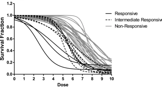
A dose-response curve (DRC) is an X-Y plot relating assay response (e.g., cell survival rate for ChemoFx) and corresponding dose [Huang and Pang,2008]. Figure 2provides an exam-ple of dose-response curves from ChemoFx assay [Suchy et al., 2011].
Figure 2: Dose response curves (DRCs) of the breast specimens treated with sunitinib. Responsive (R) specimens are denoted with a solid black line 3/39 (7.6%), intermediate responsive (IR) specimens are delineated with a dashed black line 8/39 (20.5%) and non-responsive (NR) specimens are indicated by a gray line 28/39 (71.7%)
For the baseline adjustment of the DRCs, the control well mean (CWM) for a patient is defined as the mean cell counts in the untreated wells:
CW M i = 1 M M X m=1 Xi,m0 (2.1)
Where M represents number of dose-0 wells for each patient, and Xi,m0 represents the cell counts from each dose-0 well. Since nine drugs are usually tested on one plate, with each measurements repeated three times, the maximum of M is 27 based on the assay design. But in practice M varies because of the possible failure of assays or insufficient cells for all of the treatment.
Dose response (DR) at dosek is then defined as the cell survival fraction using the mean of cell counts from different wells at dose-k divided by the CWM for a patient i:
DRi,j,k = Yk
i CW Mi
, k = 1,2, . . . ,10. (2.2)
where mean cell counts at dose-k is the average of the three reps, as Yk
i = 1 3 P3 p=1Y k i,p.
A DRC describes the change of cell-killing percentages with the increasing drug concen-trations for each treatment option. The goal is to assess the tumor cells in vitro sensitivity to each of the clinical treatment options, this is then used to predict the patient’s clinical response to the treatments and thus help physicians in making treatment decisions.
In practice, investigators usually use a two-stage approach for classification based on DRCs [Huang and Pang, 2008]. In the first stage, summary statistics are extracted from each DRC, with choices of methods including half-maximal inhibitory concentration (IC50), area under dose-response curves (AUC). In the second stage, the summary statistics extract-ed from the first stage and other baseline variables are usextract-ed to prextract-edict clinical response.
The half-maximal inhibitory concentration (IC50) and area under does response curves (AUC) are both common choices of traditional methods for extracting summary statistics from the dose-response data from assay experiments [Huang and Pang, 2008].
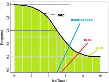
Absolute IC50 is defined as the concentration which generates half of the maximal effect - mid-point between the max effect and zero [Cheng, 2002]. Relative IC50 is similar to absolute IC50 except that the maximal effect is adjusted by a baseline (minimal effect)- the mid-point between the max effect and the min effect. The difference between absolute IC50 and relative IC50 can be demonstrated in Figure 3.
In in vitro dose-response assays, IC50 is the most widely used metric to analyze DRCs, and it is usually estimated based on a parametric approach. For a given drug, assays with a larger IC50 suggests that the tumor cells are more resistant to the drug.
The area under the DRC, a.k.a. AUC, is another common method for quantifying dose-response curves and used for curve comparisons [Mi et al., 2008]. It is defined as the sum of
Figure 3: Definition of IC50, relative IC50 and AUC on a DRC. DR at dose from 1-10: AU C = 10 X k=1 DRk (2.3)
AUC method is used to quantify the relative height of the DRCs. When comparing the DRCs of two patients treated with the same drug, the lower DRC suggests that the tumor cells of that patient is be more sensitive to the drug. The convenience of interpretation of AUC in predicting clinical response is a great advantage of the method.
Truncated or partial AUC is a modification of AUC method. The motivation for this approach is that during the model training it is found that not all of the concentrations are informative (correlated with) the clinical outcome. AUC7, for example, computes the AUC using DRs at dose from 1-7, considering that the growth of tumor cells under high concentration (dose 8-10) may not be distinguished for different drugs.
AUC and IC50 both reduce the dimension of the DR data from 10 to one (assuming that the triplicate measurements at each concentration are averaged first). This dimension
reduction may simplify the prediction model in the second stage. AUC and IC50 methods also have clear and intuitive interpretation.
When the CWMs change, IC50s will stay the same, because the calculation of IC50 de-pends on the relative change of dose-response. AUCs can be affected in that situation, and thus prediction of clinical response is also impacted. The information about the free growth of tumor cells itself is indicative of how aggressive the tumor cells are, and it should be in the prediction model.
As usual, there could be loss of information in the dimension reduction process when only IC50 and AUC are used to summarize the dose-response data. For example, as shown in Figure4, two dose-response curves have the same AUCs and IC50s, but the chemo-sensitive kinetics might be totally different, because part of the information on the cell killing mech-anism is not captured by AUC or IC50.
To address the above concern, the DRCs should be fitted with a function that is required to not only reduce the dimension of the data, but also describe the curve kinetics. Four-parameter logistic function (4PL) is widely used for fitting DRCs in industry. The 4PL function is defined as in [Huang and Pang, 2008]:
y=β2+
β1−β2
1 + (β4
x)β3
(2.4)
Here,β2 denotes upper plateau,β1denotes lower plateau, β3denotes slope/speed of response
to dosage change, and β4 denotes IC50.
An alternative version of 4PL function could be used[Ritz and Streibig,2005]
y=β2+
β1−β2
1 +eβ3(β4−x) (2.5)
In this form of four parameter logistic model,β1,β2 and β3 will be similar to that in formula
(2.4); β4 and x here will be similar to log(β4) and log(x) in formula (2.4), considering the
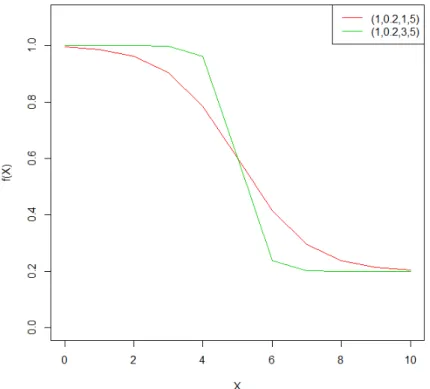
Figure 4: Four-parameter logistic function (4PL). 4PL with (β1, β2, β2, β4) = (1,0.2,1,5) is
corresponding to the red curve, 4PL with (β1, β2, β2, β4) = (1,0.2,3,5) is corresponding to
the green curve.
(2.5)taking into accountthat the dose k from1-10 represent the drugconcentrations expo-nentially increasing with base 10.
InFigure4,the 4PLfunctionofindex dosagexfrom0to10areplottedundertwo setups ofparameters.β4=5wassetforbothcurves,thismeansthatbothcurveshaveIC50=5(i.e.,
the dose x wherederivative of f(x) reachesmaximum). By settingβ1=1 and β2= 0.2, both
curves start from cell survival proportion 1 and end with 0.2. By setting β3 = 3 (red) or 5
(green),theyhavedifferentslopesatdosex=5.
AsinterpretedwiththeplotofDRCs,eachparameterinthe4PLfunctionhasexplicit meaningintheinterpretation.OncetheDRCisfittedwith4PLfunction,theparameters may
4PL model reduces the dimension of the DR data from 10 to 4, it preserves more in-formationregardingdose-responsemechanismthanAUC orIC50alone.Generally,whenthe drug concentrationsare welldesigned and the noise levelis well controlled(so thatthe data complieswiththe4PLmodelfittingassumptions),the4PLmodelperformsbetterthanusing onlythehighest3dose-responses[HuangandPang,2008].
2.2 THE PROPOSED METHODS FOR CLASSIFICATION BASED ON
DOSE-RESPONSE DATA
2.2.1 Five-parameter mixture of exponential function (5ME) method
The 4PL model is a useful functional form that describes DRC’s with flat top and bottom (low and high dosage). However, in reality such low/high-dose plateaus do not always exist, it is then a mathematical challenge to estimate the IC50 if the DRC does not comply with the model fitting assumptions. Illustrated in Figure 5, specimens from National Surgical Adjuvant Breast and Bowel Project (NSABP) B-40 trial with patients treated by T+AC without Bev. In ChemoFx assay experiment, the DRCs using doxorubicin (drug A) usu-ally does not have flat beginning and ending. Biologicusu-ally, such two-phased exponentiusu-ally decreasing trend in DRCs is not uncommon and quite often the cause is unknown; in this case, it could be caused by the mixture of tumor cells and fibroblast cells in the specimens. Therefore, another functional form is needed to fit this type of unusual DRCs with steep ends.
Here we propose a five-parameter mixture of exponential function (5ME) method for dose response curve fitting. The 5ME function consists of two different exponential decreasing components:
Figure 5: Mean of DRCs of the breast specimens treated with doxorubicin (A). Specimens from pathological complete response (pCR) groups are corresponding to the red line, speci-mens from non-pCR groups are corresponding to the black line.
where x denotes the dosage, (a, b, c, d) are parameters describing the dose-response mech-anism of the DRC: Under lower dosage, we assume that the DRCs start with a fast drop and slow down as f(x) = e−dx; Under higher dosage, we assume that the DRCs start with a slow drop and accelerate the decreasing as f(x) = 1−ebx. ρ denotes a weight
parame-ter for how much proportion of the DRC is shared by each component of exponential function.
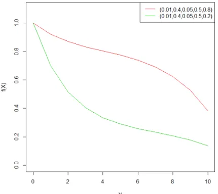
In Figure 6, we present plots of 5ME functions under two setups of parameters. Param-eters (a,b,c,d) are set as the same for both curves, which means that the 2 components of exponentially decreasing function are exactly the same for both curves. We set the weight
Figure 6: Five-parameter mixture of exponential function (5ME). 5ME with (a, b, c, d, ρ) = (0.01,0.4,0.05,0.5,0.8) is corresponding to the red curve, 5ME with (a, b, c, d, ρ) = (0.01,0.4,0.05,0.5,0.2) is corresponding to the green curve.
parameter to be ρ = 0.8 or 0.2, such that the two curves have different proportions of the two exponential functions. The red curve consists of 80% of f(x) = 1−ebx and 20% of f(x) = e−dx, whereas the blue curve consists of 20% off(x) = 1−ebxand 80% off(x) = e−dx. Similar as 4PL method, after the nonlinear curve fitting, the estimated parameters can be used as inputs of the prediction model for patients’ chemotherapy sensitivity.
Compared with non-parametric methods, parametric curve fitting methods such as 4PL and 5ME focus more on the dose-response mechanism when extracting summary statistics from DRCs. If the mechanisms agree with the model assumptions, parametric curve
fit-ting should outperform the non-parametric methods. On the other hand, non-parametric models such as AUC and non-parametric IC50 are less sensitive to the violation of the model .
2.2.2 Branching process using dose-0 cell counts data
As discussed earlier, the sample size of dose-0 cell counts in ChemoFx assays usually varies from 6 (2 drugs) to 27 (9 drugs). The mean of the dose-0 cell counts, CWM, is used for the standardization of DRCs. The dose-0 cell counts data are usually not used in predict-ing patients’ chemotherapy sensitivity. Even if the baseline information is used, oftentimes people only consider the mean but ignore the variance. Simply adding mean and variance of dose-0 cell counts may improve the prediction of patient chemo-sensitivity, but extracting cell growth characteristics from the dose-0 cell counts data could benefit us more in predic-tion and model interpretapredic-tion. Here we propose a branching process method for extracting information on the uninhibited growth of tumor cells from dose-0 cell counts data. By setting up a proper stochastic process model for cell growth in an assay, we can compute patient specific characters such as initial cell count in the well, cell division probability, and the number of cell cycles with a fixed time window.
A branching process models the reproduction of particles such as cell proliferation. A branching process assumes each particle follows the same probability/rule to produce off-spring, and there is no interaction between any particles [Lange, 2010]. Time is measured discretely as generations in a branching process. Here we assume a cell division process following a Bernoulli distribution.
At time zero of ChemoFx assay, tumor cells are placed in assay plates and are allowed to grow with or without inhibition for 72 hours. The initial cell counts in wells are unknown. The assay protocol requires that 320 cells are placed in each well, but this number varies due to technical variability. Since a typical cell cycle takes 24 hours, we assume that all cells have experienced three cell cycles. We denote:
Figure 7: Branching Process: free growth and drug effect
W0 (TBD): the number of cells initially placed in a well at time zero;
W0
t (measured): the number of cells in the well 72 hours after time zero, no treatment
was applied;
Wtk (measured): the number of cells in the well 72 hours after time zero, treatment of dose-k was applied;
p (TBD): the probability of division in each cell cycle;
n = 3: the number of cell cycles experienced in time duration [0,t], here t= 72 hours.
For each patient, the original assay cell counts data are composed of, (W0
t, Wtk),
mea-sured in triplicates, for each treatment. Usually Wt0 has more than 20 replicates and Wtk
has 3 replicates for each k. We are interested in the patient specific parameters (W0,p) that
describes the free growth character of patients’ tumor cells. For a given patient, W0 reflects
how healthy the tumor cells are because the true starting number of cells for each patient depends on the surviving proportion of cells when they are plated;preflects how aggressively the tumor cells grow.
As shown in Figure 7, for cell growth without inhibition, the branching process is as-sumed to follow a Bernoulli distribution with probability of division p . The probability of killing q is only applicable to drug-treated wells. Based on the branching process [Lange,
2010], for the free growth starting from one cell, we have:
µ=E(Yt0) = (1 +p)n
σ2 =V ar(Yt0) = (1−p)(1 +p)n−1[(1 +p)n−1]
Starting from W0 cells:
W0 = W0 X j=1 Y0j = W0 X j=1 1 Wt0 = W0 X j=1 Ytj0
Suppose that W0 is a random variable with mean µW and variance σW2 , then conditioning
onp and n we have the mean ofWt0:
E[Wt0|p, n] =EW0[E[ W0 X j=1 Ytj0|W0, p, n]] =E[(W0|p, n)µ] =µWµ E[Wt0|p, n] =µW(1 +p)n (2.7)
Similarly we have conditional variance ofWt0:
V ar[Wt0|p, n] =V arW0[E[ W0 X j=1 Ytj0|W0, p, n]] +EW0[V ar[ W0 X j=1 Ytj0|W0, p, n]] =V ar[(W0|p, n)µ] +E[(W0|p, n)σ2] =σW2 µ2 +µWσ2
V ar[Wt0|p, n] =σW2 (1 +p)2n+µW{(1−p)(1 +p)n−1[(1 +p)n−1]} (2.8)
Note that our data is only consisted of the dose response well counts after-treatment : {W01
t , Wt02, Wt03, . . . , Wt0 M}for dose-0 cell counts (M is the number of replication of dose-0
wells) and {Wtk1, Wtk2, Wtk3} for dose-k cell counts (k=1,2,. . . ,10). For patient i, we have:
E(Wt i0 ) =µW i(1 +p0 i)ni
E(Wt ik ) =µW i(1 +p0 i(1−2qk i))ni
Because the variance of Wk
t i can not be reliably estimated due to the small sample size
(at most three), here we apply the branching process model only to dose-0 cell counts data to solve for free growth characters (µW, σW2 ,p) for each patient.
By setting n = 3, here we have three unknown parameters (µW, σW2 , p) and two (mean
and variance) equations (2.7)(2.8), therefore we must add assumptions/constraints on (µW, σ2
W, p and/orn). Here are some tentative choices:
If the variance is assumed to be σW2 for the initial cell counts W0, we may compute the
mean well counts at initial time µi
W and cell division probability pi for each patient i.
Alternatively, if a Poisson distribution of W0 can be assumed that W0 i ∼ P OI(λi), we
have
E[Wt i0 |p, n] =λi(1 +pi)ni
V ar[Wt i0 |p, n] =λi(1 +pi)2ni+λi{(1−pi)(1 +pi)ni−1[(1 +pi)ni −1]}
then we will have cell division probability and initial cell counts (pi, λi) solved for each pa-tienti.
Similar to 4PL and 5ME, the parameters derived from modeling dose-0 cell counts data using branching process have explicit meanings, and they are then used as inputs to the prediction model for patient clinical response. For example, if we assume Poisson distribu-tion ofW0, we may have (pi, λi) used as inputs in the prediction of patients’ clinical response.
2.3 SIMULATION STUDIES
2.3.1 Comparing 5ME, IC50, and AUC using simulated cell counts data
In this simulation study we generated cell counts data from a mixture of two branching process to simulate the growth of the mixture of fibroblast cells and tumor cells. In each simulation we generated data for 300 patients, 100 labeled with pathological complete re-sponse (PCR) and the remaining 200 labeled with non-PCR. For a patient i, 10 dose-0 cell counts and 3 dose-k (k=1,. . . ,10) cell counts were generated. Initial cell counts W0
were generated from W0 ∼ P OI(Z), where Z ∼ N(300,502), with the ratio of tumor cells
r ∼ U N IF(0.7,0.9). Fibroblast cell killing probability qF(k) and tumor cell killing
proba-bility qT(k) (qT+ for pCR group andq
−
T for non-pCR group) follows:
qF(k) = 1−exp{−0.5k} qT+(k) = 0.4 + 0.5
1 + exp{0.7(7−k)}
qT−(k) = 1
1 + exp{1.2(6.5−k)}
The mean DRC are presented in Figure 8. Here we chose not to generate the dose-response data following an exact 5ME function (in fact a 4PL+ exponential function form was used) because 5ME model is expected to be flexible in fitting DRCs and show its ad-vantage in prediction. After each simulation, with the 300 patients’ dose-0 and dose-k well counts, CWM for each patient was computed and used to standardize the DRCs, then we applied the proposed 5ME method and existing methods such as AUC and IC50 to extract
Figure 8: Mean DRCs of simulated cell counts data.
summary statistics from the DRCs. We separated the inputs into training set and testing set (ratio as 4:1) and used a logistic model to predict pCR. The process was repeated for 1000 times. Mean and empirical standard deviation of sensitivity, specificity, PPV, NPV, and prediction accuracy were computed and compared for each method.
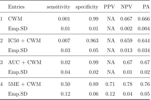
The simulation results are shown in Table 1. TheN A0sin PPV column for CWM, IC50 and AUC methods are caused by some extreme predictions of pCR by using these methods
when all patients in testing set are predicted resistant to chemodrugs. Under the given set-up of parameters, CWM, IC50 and AUC do not differ between two groset-ups. Therefore the logistic models using CWM, IC50 or AUC did not provide good prediction of chemosensitiv-ity. The 5ME curve fitting method in this case can transform the data into the parameter space and tell the difference between the two groups. Although we choose not to use 5ME function to generate the data , the method still show its advantage. The prediction accura-cy using 5ME method is significantly better than those using CWM, IC50 and AUC methods.
Table 1: Comparison of 5ME, IC50 and AUC based on simulated cell counts
Entries sensitivity specificity PPV NPV PA
1 CWM 0.001 0.99 NA 0.667 0.666 Emp.SD 0.01 0.01 NA 0.002 0.004 2 IC50 + CWM 0.007 0.963 NA 0.659 0.644 Emp.SD 0.03 0.05 NA 0.013 0.034 3 AUC + CWM 0.02 0.99 NA 0.67 0.67 Emp.SD 0.04 0.02 NA 0.01 0.02 4 5ME + CWM 0.50 0.89 0.71 0.78 0.76 Emp.SD 0.12 0.06 0.12 0.04 0.05
2.3.2 Comparing 5ME, IC50, and AUC using simulated dose-response curves
In this simulation study, instead of generating the cell counts from mixture of branching pro-cesses, here we repeatedly (K=1000) simulated the proportion of cell surviving from some given functions and artificially adding some errors. Here we generated the dose response curves from a seven-parameter mixture of an exponential function and a logistic function (7MEL):
f(k) = ρ · {a + b−a
1 +exp(c(d−k)))} + (1 − ρ) · {A + (1 − A) · exp(−Bk)} + (2.9) where ∼U N IF(−0.1,0.1).
As presented in Figure 9, in each simulation we generate dose-response data following 7MEL function as in (2.9), and eight different setups of parametersθ = (a, b, c, d, A, B, ρ) as
θ1+= (1,0.2,3,5,0.5,0.5,0.4) θ1−= (1,0.2,1,5,0.5,0.5,0.4) θ2+= (1,0.2,3,4.5,0.5,0.15,0.4) θ−2 = (1,0.18,1,4.7,0.4,0.1,0.44) θ3+= (1,0.2,3,5.6,0.4,0.15,0.3) θ−3 = (1,0.3,1,6,0.5,0.3,0.44) θ+4 = (1,0.1,3,8,0.4,0.15,0.3) θ−4 = (1,0.2,1,8,0.5,0.3,0.44)
Table 2: Comparing 5ME, IC50 and AUC using simulat-ed dose-response data
Entries sensitivity specificity PPV NPV PA
1 IC50 0.61 0.49 0.56 0.57 0.55 Emp.SD 0.19 0.20 0.05 0.05 0.02 2 AUC 0.71 0.55 0.61 0.65 0.63 Emp.SD 0.06 0.07 0.03 0.05 0.04 3 5ME 0.79 0.56 0.64 0.73 0.67 Emp.SD 0.06 0.06 0.03 0.05 0.03
(a) 7MEL functions withθ+1 andθ1− (b) 7MEL functions withθ+2 andθ2−
(c) 7MEL functions with θ+3 andθ−3 (d) 7MEL functions withθ+4 andθ4−
Figure 9: Mean of Simulated DRC following seven-parameter mixture of a 4PL function and an exponential function (7MEL) functions.
Among the eight setups of parameters, we use θ+1, θ2+, θ+3, and θ+4 for generating DRCs for sensitive patients, and θ−1, θ2−, θ3−, and θ−4 for generating DRCs for resistant patients. We generate 9600 DRCs (1200 for each θ), split them into training set and testing set in a 5:1 ratio, and apply the proposed 5ME methods and traditional methods such as IC50 and AUC. We repeated the process forK = 1000 times. Mean and empirical standard deviation of sensitivity, specificity, PPV, NPV, and prediction accuracy were computed and compared for each method.
Table 2summarizes the performance of these methods using dose-response data simulat-ed from 7MEL functions. Here since we set the parameters θ’s in pairs such that the AUC and IC50 are similar between the sensitive and the resistant groups, the prediction accuracy is relatively low as we expected. Compared to IC50 and AUC, the proposed 5ME method shows better performance predicting responses in such a mixture pattern situation.
2.4 APPLICATION TO CLINICAL TRIAL DATA
2.4.1 Analysis of B40 trial data
National Surgical Adjuvant Breast and Bowel Project (NSABP) Protocal B-40 was designed to determine if adding capecitabine(X) or gemcitabine(G) to neo-adjuvant docetaxel followed by doxorubicin/cyclophosphamide(T+AC) and if adding bevacizumab(Bev) to chemothera-py would improve pathologic complete response(pCR) rate of breast cancer patients.
Pathologic complete response(pCR) is defined as no invasive and no in situ residuals in breast and nodes for breast cancer patients [Minckwitz et al.,2012]. pCR can be associated with patient disease free survival (DFS) after treatment. For some subgroup of patients, pCR can be used as a suitable surrogate end point.
It was learned from another neoadjuvant trial conducted and reported by NSABP, proto-col B-27, that adding docetaxel(T) after doxorubicin/cyclophosphamide (AC) significantly increased clinical and pathological response rates for operable breast cancer [Bear et al.,2003,
2006, Fisher et al., 1997]. Recent research showed that bevacizumab(Bev) and capecitabine (X) / gemcitabine (G) could possibly improve response rate for some metastatic-disease [Robert et al., 2011, O’ Shaughnessy et al., 2002, Albain et al., 2008]. Therefore NSABP protocol B-40 trial followed such factorial design that eligible patients were randomly as-signed to 3 arms T+AC, TX+AC, and TG+AC, then patients in each arm were randomized to receive Bev or not(see Figure 10).
At the end of B-40 trial, 1186 of the 1206 patients had available pCR data. The con-clusion from analysis of B-40 clinical data was that addition of X or G did not significantly improve pCR rate compared with T alone (pCR rate in Arm 2 and 3 was not significantly higher than that in Arm 1); addition of Bev to chemotherapy significantly increased pCR rate (pCR rate in Arm B’s was significantly higher than that in Arm A’s)[Bear et al.,2012]. For patients with positive hormone receptor(HR), the effect of adding Bev was significant, while for patients with negative HR, the effect was minimal.
In B40 trial, the biopsies from breast cancer patients were delivered to ChemoFxR
as-say lab in Precision Therapeutics Inc. for ex vivo experiments. Tumors cells were cul-tured for several weeks until they reached the requirements for assays in both quality and quantity. Then each patient’s cells were placed by robots into wells on plates to receive all single drugs and combinations of those drugs (11 assays for B40 in total: T,A,C,X,G, TX,TG,AC,TAC,TXAC,TGAC).
A total of 473 patients in B40 trial had successful ChemoFx assay experiments using drug A and T, and 223 of them were involved in arm 1A, 2A, 3A (treated without Bev) and the remaining 250 were involved in arm 1B, 2B, 3B (treated with Bev). Our validation was only conducted on 223 patients from arm A and using the assay results for drug A and T. Patients from arm B were not used because Bev had been proved to significantly
improve pCR rate, which could confound the results. Drug C was also not used for analy-sis because there is evidence from the lab that the assay results for this drug were not reliable.
(a) Sample DRC by pCR, drug A (b) Sample DRC by pCR, drug T
Figure 11: Sample dose-response curves in assay with drug A or T, grouped by pCR of patients in NSABP B-40 Arm 1A.
Figure shows some sample individual DRCs in assay with drug A and T for patients from arm A1 where T+AC was applied. Unfortunately the mean DRC of patients with pCR was even higher than that of patients without pCR based on assay results of drug A, which was the opposite of what we expected. The mean DRCs of patients with pCR and non-pCR were also not separable based on assay results of drug T, adding into the difficulties of predictions.
The DRCs were standardized by the CWMs. For extracting summary statistics, we ap-plied AUC7, AUC10, IC50, BP and parametric curve fitting (4PL method for assay using drug T and 5ME for assay using drug A). We fitted drug A and drug T assays with different models, because drug T showed DRCs with high and low plateaus, while drug A assays could only be fitted by 5ME model. The summary statistics from drug A assays and drug T assays are combined and used as inputs for prediction. We applied 5-fold cross-validation
(a) Mean DRC by pCR, drug A (b) Mean DRC by pCR, drug T
Figure 12: Mean dose-response curves(DRC’s) in assay with drug A or T, grouped by pCR of patients in NSABP B-40 Arm 1A.
for K = 1000 times using logistic model to predict patient pCR. The prediction accuracy and corresponding resampling standard error of these methods are summarized in Table3.
Table 3: Comparison of methods using B40 ChemoFx assay data
Method NO.pts Prediction Accuracy Resampling SE
1 DRC + CWM 223 0.67 0.09 2 AUC10 + CWM 223 0.71 0.14 3 AUC7 + CWM 223 0.65 0.09 4 IC50 + CWM 223 0.69 0.07 5 4PL/5ME+CWM 222 0.70 0.13 6 4PL/5ME+BP 198 0.68 0.07
To compare the methods 1-5, with logistic models using different inputs such as dose-response data, AUC10, AUC7, nonparametric IC50, or 4PL/5ME, IC50 appeared to have a smaller resampling SE, and a slightly better prediction accuracy. The 4PL/5ME method showed a higher prediction accuracy, but the resampling SE was also larger. This was proba-bly caused by the large noise of the dose-response data, and because parametric models have more parameters, the variation of prediction performance could be more affected compared to simple model such as non-parametric IC50. AUC10 also showed a large SE in prediction, this could be caused by the instability of the responses at higher doses.
To compare methods 5 and 6, with 4PL/5ME approach with or without character vari-ables from branching process in the model, branching process did not provide any improve-ment in predicting pCR, this method was also unable to achieve a solution ofpfor 24 patients.
2.4.2 Analysis of PTI-206 ChemoFxR assay data
To further validate the performance of the proposed branching process (BP) method, herein we conducted the analysis using PTI-206 assay data. PTI-206 was a study for advanced ovarian cancer. In the study, patients were enrolled in a pre-defined protocol. Tumor sam-ples from 54 institutions were submitted for chemo-response testing between 2006 and 2010. Women with FIGO stage III-IV epithelial ovarian (EOC), fallopian tube (FTC) and peri-toneal (PPC) cancer treated with carboplatin (C)/ paclitaxel (P)-based chemotherapy fol-lowing initial cytoreductive surgery were included in the study. Clinical response (CR) was defined as positive if a patient experienced more than six months from the end of primary chemotherapy. If recurrence was reported within six months, then the patient had no CR.
262 patients in the PTI-206 trial had successful ChemoFx assay results. After filtering out missing data, 230 patients remained with clinical response (CR) and Carboplatin assay
result (Carboplatin is the drug applied to patients in this trial). The goal of this applica-tion is to compare the BP with tradiapplica-tional baseline adjustment methods in predicting CR. AUC7 is used for the prediction in these Chemofx assays, considering the instability of assay responses at high doses.
For each patient, the data to be used includes AUC7, CWM and dose-0 cell counts. To apply the BP method, we first computed the mean and variance of dose-0 cell count. Then assuming all cells experiencing three cycles in 72 hours in the assay experiment (n = 3) and Poisson distribution for initial well counts (W0 ∼P OI(λ)), we used (2.7,2.8) to compute the
initial mean cell counts λ and cell division probability p for each patient.
To predict CR, logistic models are performed with the following inputs: CWM + vari-ance of dose-0 counts, λ + p, AUC7 + CWM + variance of dose-0 counts, AUC7 + λ +
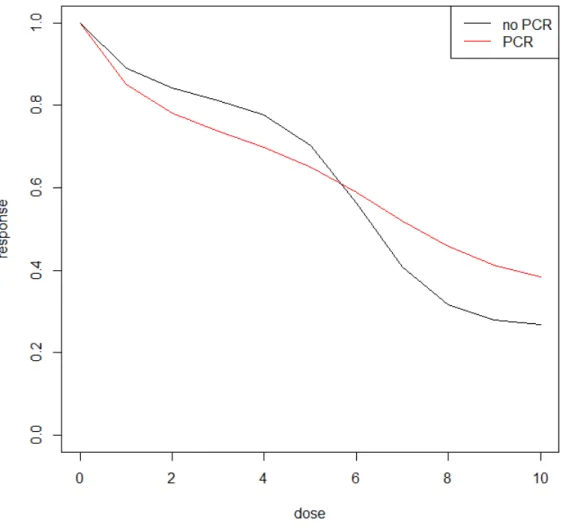
p. The performance of prediction was compared by receiver operating characteristic (ROC) analysis. The ROC plots are shown in Figure 2.4.2. The Area under the ROC curve (AU-ROC) of each method are summarized in Table 4. AUROC for CWM + variance of dose-0 counts model was 0.617, AUROC for λ + p model was 0.628, AUROC for AUC7 + CWM + variance of dose-0 counts model was 0.632, AUROC for AUC7 + λ +p model was 0.647.
Table 4: Comparison of methods by AUROC based on PTI-206 assay data
Predictors AUROC
1 mean and variance of dose-0 cell counts 0.617
2 (λ, p) from BP 0.628
3 AUC7 + mean and variance of dose-0 cell counts 0.632
(a) Inputs: CWM + variance of dose-0 counts (b) Inputs: λ+p
(c) Inputs: AUC7 + CWM + variance of dose-0 counts
(d) Inputs: AUC7 +λ+p
First, we compared model 1 and model 2 (CWM + variance of dose-0 counts model vs λ
+ pmodel). The inputs in these two methods were equivalent in information, because that
λ + p was computed from CWM + variance of dose-0 counts by using BP method. In this comparison, the BP method improved the AUROC by 1.8%.
We then compared model 3 and model 4 (AUC7 + CWM + variance of dose-0 counts model vs AUC7 +λ + pmodel). The inputs in these two methods were also equivalent. In this comparison, the BP method improved the AUROC by 2.4%.
2.5 DISCUSSIONS
Here we proposed a five-parameter mixture of exponential function (5ME) method for dose-response curve (DRC) fitting and a branching process (BP) method for dose-dose-response baseline characterization.
The 5ME model is a parametric curve fitting method similar to the four parameter lo-gistic model (4PL). The difference between these two models is the type of dose-response curves they describe. The 5ME model can be fitted into DRCs without upper and bottom plateau, and an improved performance is seen in simulation study by comparing with other traditional methods such as IC50 and AUC.
When noise is large as that in the B40 assays, the fitting of 5ME function to DRC is not precise, and the prediction performance using the curve parameters is than ideal.
The BP method is based on the cell division modeling in an in vitro assay. This method was illustrated in the analysis of PTI-206 assay data. When applying this model, because the variance of dose-0 cell counts were utilized, it was expected to provide more information on the character of patient’s tumor cells. Compared to using mean and variance of dose-0 cell counts, usingλandpfrom the BP method improved the prediction of clinical response.
The improvement by the branching process method, relies on the available biological knowledge of cell division process in assay experiment. Here we simply assumed that the number of cell cycles was fixed and the probability of cell division followed a Bernoulli prob-ability. These assumptions can be refined and the prediction should be improved if we have more understanding of the experiment and the behavior of tumor cells in the assays, such as the distribution of initial cells in each well and the cell cycle variation.
3.0 A MODIFIED EM ALGORITHM FOR REGRESSION ANALYSIS OF DATA WITH NON-IGNORABLE NON-RESPONSE
3.1 OVERVIEW OF ANALYSIS OF MISSING DATA
3.1.1 Missing data in practice
Missing data are prevalent in biomedical studies especially in large clinical trials and longi-tudinal studies where values of some variables are missing from many subjects. In general, missing values may occur due to design, loss to follow-up or inability to record [Little and Rubin, 2002] [Little et al.,2012].
For example, in some case-control studies, the assessment of a bio-marker is too expen-sive that the investigators can only afford to perform the assay on a subset, or values of certain exposure variables may not be available from some subjects based on their existing records. In many longitudinal studies, an outcome variable is repeatedly measured over time to provide information on its trend overtime in individuals. The values of the outcome vari-able may be missing during the study because of missed visits or dropouts.
In most statistical software packages, subjects with missing values are deleted automati-cally and analysis is solely based on the subsets with complete records on involved variables. Simply applying standard statistical methods using complete cases often leads to biased es-timates. The bias can be substantial when the proportion of missing values is high or the missingness does not occur randomly. Missingness in some variables may cause imbalance in treatment among the complete cases. For example, in a randomized clinical trial, patients
are randomized into two treatment arms, to balance the two groups for both known and unknown factors. If patients’ dropout is related with less improvement of the symptoms than expected, then the comparison between the treatment groups will be biased in favor of higher rate of dropout.
It is important to distinguish missing-data patterns and missing-data mechanism because of their implication in appropriate statistical analysis[Little and Rubin,2002]. Missing-value indicators, with value at 1 or 0, are often used to indicate the missing status of a variable for a subject. Then we have a vector for each subject and a matrix of missing indicators for all subjects. Such missing indicator matrix forms the missing-data pattern. Missing-data patterns are used to describe which values are observed and which values are missing. For example, monotone missing data are related with longitudinal dropouts, when all future ob-servations are missing after the dropout. Non-monotone missing data are more complicated and require modeling of the dropout mechanism.
Missing-data mechanism is used to describe how missingness is related with the hypo-thetical complete data, including missing values. Rubin [Rubin, 1976] defined three types of missing-data mechanisms: missing completely at random (MCAR), missing at random (MAR) and not missing at random (NMAR). When missingess is not related with the values of any variables in the study/data, the data are called MCAR. When missingess is related with the values of observed variables only, the data are called MAR. When missingess is related with the values of unobserved variables after conditioning on the observed variables, the data are called NMAR.
For example, in a randomized clinical trial with two treatment arms, suppose that pa-tients in treatment group will receive IV injection, whereas those in control group will take pills. If a patient discontinues the treatment because he does not like the flavor of the pills, the missing mechanism here is MAR. This is because that the group assignment is observed. If loss of follow-up is caused by heart attack which is only related to real-time blood pres-sure, then the missing-data mechanism is NMAR. This is because that the values which
missingness depend on may not be observed. If loss of follow-up is caused by relocation for job change, the data are in general MCAR.
3.1.2 Statistical methods for analysis of missing data
In the following context, we denote Y = (Y1, . . . , YK) the vector of variables and R =
(R1, . . . , RK) the vector of missing data indicators. Y = (Yobs, Ymis), Yobs and Ymis denote
the observed and missing components of Y.Rk= 0 ifYkis missing; Rk = 1 ifYk is observed.
Missing-data mechanism is generally described via conditional distributionf(R|Y, ψ), where
ψ denotes parameters for the missing-data mechanism model. Based on how the missingness is related to the hypothetical complete-data vector Y, Rubin classified three missing-data mechanisms [Rubin, 1976]:
1. MCAR
Data are missing completely at random(MCAR) if the missingness does not depend on the underlying complete data at all.
f(R|Y;ψ) = f(R;ψ)f or all Y.
2. MAR
Data are missing at random(MAR) if the missingness depends on observed values only.
f(R|Y;ψ) = f(R|Yobs, ψ)f or all Ymis, ψ.
3. NMAR
When missingness still depends on Ymis after conditioning on Yobs, the data are called not missing at random (NMAR).
For regression analysis of a data set, missingness could happen in response, covariates, or both. The impacts of missing values are different for response and covariate, and yield different analytical methods.
In the following context, we consider regression analysis of data with nonresponse where the covariates are fully observed and the response variable is subject to missing values. Suppose the observed data for (X, Y) are {(x1, y1),(x2, y2), ...,(xn, yn)}, where x0is are
ful-ly observed, and the response variable Y is only observed for the first r subjects, i.e., (yr, yr+1, ..., yn) are missing. In practice, we are usually concerned with the following
re-gression models:
[Y|X]∼g(y|x;θ)
where g(·|x;θ) is a parametric or semi-parametric model. Here the interest is to make inference on θ. There are generally two types of methods in missing-data analyses [Ibrahim et al., 2012]: ad-hoc methods such as complete case analysis and imputations, and stan-dard statistical methods such as inverse-probability weighted estimating equations (IPWEE), maximum likelihood, Bayesian / data augmentation methods.
Complete-case analysis is a simple methods that applies on the complete cases. In complete-case analysis, the statistical inference onθ is based on the complete cases{(x1, y1),
(x2, y2), ...,(xr, yr)}. Complete-case analysis is based on a well-defined subset and simple to
perform. However, it does not use information collected from incomplete cases. It is usually inefficient and may be biased when data are not MCAR [Ibrahim et al., 2012].
Imputation is also a common ad-hoc method for analysis of missing data. In general, the imputation methods are conducted as following: at first we identify missing values from the data, then we obtain a predictive model for the distribution of missing values given observed data. Values are drawn from the predictive distribution. After imputations, the usual estimation can be performed on the imputed dataset
where ˜yj0s are the imputed values. Imputation is a straightforward and flexible method. However, appropriate imputation methods usually require a reasonable (estimated) impu-tation model. The subsequent inference has to take into account of the variations due to imputation models and the intrinsic variation due to the draws[Little and Rubin, 2002].
Multiple imputation are used to justify variation to improve single imputation. In mul-tiple imputation, we repeatedly generate D (usually 2 ≤D ≤ 10) complete data sets, then we can achieve inference on θ by combining the estimations from D data sets[Rubin, 1987] as follows: ¯ θD = 1 D D X d=1 ˆ θd (θ−θ¯D)T −1 2 D ∼tν
where TD is the variance of ¯θD computed from within-imputation variance and between
im-putation variance, ν is the degrees of freedom of the t distribution computed from D and the variances.
The advantage of multiple imputation is the computation efficiency. Compared with re-sampling methods such as bootstrap and jackknife, multiple imputation required fewer times of repeating computation to obtain variance estimates of imputation estimates.
In summary, ad-hoc methods usually require data missing completely at random (M-CAR) or missing at random (MAR), which limited the usage of such methods.
A generalized estimating equation (GEE) is used to estimate the parameters of a gener-alized linear model with a possible unknown correlation between outcomes[Liang and Zeger,
1986]. The inference on θ could be done by solving the follow equation:
n X
i=1
whereDi(x), θis ad×K matrix chosen according to the distribution ofyi,dis the dimension
of parameter θ,µ(x, θ) = E[Y|x].
Rubin and others presented the GEE method for the data missing at random (MAR) using inverse probability weight (IPW) [Robins et al., 1994]. When we consider the missing in data, the GEE based on the complete cases is:
r X
i=1
Di(xi, θ){yi−g(xi, θ)}= 0
where the first r yi’s are observed. Supposed there is a fully observed auxiliary variable Z.
Assuming data are MAR
pr(Ri = 1|xi, yi, zi) = pr(Ri = 1|xi, zi;ψ) =f(xi, zi;ψ)
Using inverse-probability weight [Fitzmaurice et al.,1995], the inference onθcan be achieved by solving the weighted GEE:
r X
i=1
f(xi, zi; ˆψ)−1Di(xi, θ){yi−g(xi, θ)}= 0
where ˆψ is usually estimated by regression ofR on X and Z.
GEE is a well-established method, flexible for correlation structure adjustment. [Troxel et al., 1997] extended GEE method for analysis of data with non-ignorable nonresponse. However in general GEE methods are limited to data MAR or MCAR and the missing-data mechanism is required in the likelihood function.
Likelihood-based methods can be classified into selection models and pattern-mixture models by the way of likelihood partition. Selection models [Diggle and Kenward, 1994] factor the joint distribution into underlying complete data distribution and missing data mechanism:
Pattern mixture model [Little, 1994] stratify the data based on missing-data pattern:
p(Y, R;θ, ψ) = p(Y|R;θ)p(R;ψ)
Selection model is a natural way of factoring the model considering that the relationships between Y and X in the full population is usually of interest. Also it will be shown later in this section that when data are MAR, modeling missing-data mechanism is not necessary for likelihood-based inference for selection models.
Pattern-mixture models, on the other hand, can be more suitable if the subpopulation distribution is of interest. Also in some special situations, when data are NMAR, pattern mixture models could be more convenient to perform than selection model.
Rubin showed that when data are missing at random (MAR) and missing-data mecha-nism is distinct from the regression model, the missing-data mechamecha-nism can be ignored in the likelihood-based inference [Rubin,1976]:
Lf ull(θ, φ;Yobs, R) = Z
f(Yobs, Ymis;θ)f(R|Yobs, Ymis,;φ)dYmis
=
Z
f(Yobs, Ymis;θ)f(R|Yobs;φ)dYmis
=f(Yobs;θ)f(R|Yobs;φ)
=Lign(θ)f(R|Yobs;φ)
where Lign(θ) = f(Yobs;θ) is the ignorable likelihood function. For data MAR, since the
second term in full likelihood becomes irrelevant to θ, inference based onLf ull(θ, φ;Yobs, R)
is equivalent to inference based on Lign(θ), and the missing-data mechanism does not need
to be modeled here.
When the MAR condition is not met, missing-data mechanism is required in construct-ing full likelihood function for estimation and inference of regression parameters. Mis-specification of missing-data model often yields biased estimates and wrong conclusions.
In practice, it is often the case that we can not identify the missing-data mechanism. Therefore, when applying likelihood based method for data missing not at random (NMAR), people usually make some assumptions about the missing-data model. This is the motiva-tion of the article to develop a general (missing-data mechanism assumpmotiva-tion free) method for regression analysis when missing-data mechanism is unknown.
Tanner and Wong showed that the posterior distribution of regression parameter given observed data can be achieved by an iterative data augmentation procedure [Tanner and Wong, 1987]. In the imputation step (I-step), the missing values are drawn from the dis-tribution of missing values given observed values and given regression parameters In the posterior step (P-step), the distribution of regression parameters are updated by the pos-terior distribution of model parameters derived from the imputed dataset. This method is called data augmentation.
For example, when data are MAR, Bayesian inference is based on the posterior distribu-tion
p(θ|Yobs)∝p(θ)f(Yobs;θ)
wherep(θ) is the prior distribution. A random sample are drawn from the posterior distribu-tion ofθ and its sample property can be used to make inference onθ. However, the posterior distribution p(θ|Yobs) could be complicated. By data augmentation we iteratively simulates
random samples of missing values and models parameter given observed data, with 2 steps in each iteration:
I Step (imputation): draw Ymis(t+1) with density p(Ymis|Yobs, θ(t+1));
P Step (posterior): Draw θ(mist+1) with density p(θ|Yobs, Y
(t+1)
mis ) as if data were complete.
The iterations start with initial draw θ(0) from an approximation to the posterior
distri-bution of θ. As t → ∞, the iterative procedure will eventually yield a draw from the joint distribution ofp(θ|Yobs). Data augmentation methods are usually computationally intensive.
Here we focus on maximum likelihood method, for the interest of dealing with more general missing-data mechanisms. In the following context we will develop a modified EM algorithm for regression analysis of data with non-responses when missing-data mechanism unknown.
3.2 EM ALGORITHM FOR REGRESSION ANALYSIS OF DATA WITH
NON-RESPONSES WHEN THE MISSING-DATA MECHANISM IS MODELED
Assume observed data Dobs,i = (xi, Riyi, Ri) for subject i = 1,2, . . . , n. Suppose x0is be the
fully observed covariate; yi’s be partially observed responses, observed for i=1,2,. . . ,m; Ri’s
be the missing data indicator where Ri = 1 stand for observed yi and Ri = 1 for missingyi. Without loss of generality, we assume for the complete data, the conditional distribution with parameter θ follows an exponential family and canonical link.
yi|xi ∼g(yi|xi;θ)∝exp{θS(xi, yi) +h(xi, yi) +a(θ)} (3.1)
Consider the following missing-data model
pr[Ri = 1|xi, yi] =w(xi, yi;ψ)
The interest is the inference of the distribution parametersθ.
When the parameters of the missing-data mechanism is distinct from the parameters of the regression model, the likelihood function for (θ, ψ) given observed data follows
L(θ, ψ;Dobs) = n Y i=1 p(Ri, Riyi|xi;θ, ψ) = m Y i=1 g(yi|xi;θ)w(xi, yi;ψ)· n Y i=m+1 Z g(yi|xi;θ){1−w(xi, yi;ψ)}dyi
The likelihood function could also be written as L(θ, ψ;Dobs) = n Y i=1 p(Ri, Riyi,(1−Ri)yi|xi;θ, ψ) p((1−Ri)yi|Ri, Riyi, xi;θ, ψ) = n Y i=1 p(Ri, yi|xi;θ, ψ) p((1−Ri)yi|Ri, Riyi, xi;θ, ψ) = n Y i=1 g(yi|xi;θ)p(Ri|xi, yi;ψ) p((1−Ri)yi|Ri, Riyi, xi;θ, ψ)
The corresponding log-likelihood function is
l(θ, ψ;Dobs)
=
n X
i=1
{logg(yi|xi;θ) + logp(Ri|xi, yi;ψ)−logp((1−Ri)yi|Ri, Riyi, xi;θ, ψ)} (3.2)
The MLE is
(ˆθ,ψˆ) = arg max
θ,ψ
l(θ, ψ;Dobs)
The expectation-maximization (EM) algorithm is an iterative algorithm that is often used to find the maximum likelihood estimate [Dempster et al., 1977]. Little and Rubin showed that [Little and Rubin, 2002]
l(θ, ψ|Dobs) =l(θ, ψ|D)−lnf(Dmis|Dobs, θ, ψ)
whereDmis is the missing data andD= (Dobs,Dmis) is the hypothetical complete data . The
expectation of log-likelihood function given a current estimate ofθ, say ˜θ, is
l(θ, ψ|Dobs) =E[l(θ, ψ|D)|θ,˜ ψ˜]−E[lnf(Dmis|Dobs, θ, ψ)|θ,˜ ψ˜] (3.3)
Denote Q(θ, ψ|θ,˜ ψ˜) = E[l(θ, ψ|D)|θ,˜ ψ˜] and H(θ, ψ|θ,˜ ψ˜) = E[lnf(Dmis|Dobs, θ, ψ)|θ,˜ ψ˜],
which yields l(θ, ψ|Dobs) =Q(θ, ψ|θ,˜ ψ˜)−H(θ, ψ|θ,˜ ψ˜).
Each iteration of the EM algorithm include an E-step and an M-step. In the E-step, given the current estimate (θ(t), ψ(t)), we need to calculate
Q(θ, ψ|θ(t), ψ(t)) =
n X
i=1