Imputing Missing Genotypes with Weighted k Nearest
Neighbors
Holger Schwender
∗, Katja Ickstadt
Collaborative Research Center 475, Faculty of Statistics, Dortmund University of Technology, Dortmund, Germany
Abstract
Motivation: Missing values are a common problem in genetic association studies con-cerned with single nucleotide polymorphisms (SNPs). Since most statistical methods cannot handle missing values, they have to be removed prior to the actual analysis. Considering only complete observations, however, often leads to an immense loss of in-formation. Therefore, procedures are needed that can be used to replace such missing values. In this article, we propose a method based on weightedk nearest neighbors that can be employed for imputing such missing genotypes.
Results: In a comparison to other imputation approaches, our procedure called KN-NcatImpute shows the lowest rates of falsely imputed genotypes when applied to the SNP data from the GENICA study, a study dedicated to the identification of genetic and gene-environment interactions associated with sporadic breast cancer. Moreover, in contrast to other imputation methods that take all variables into account when replacing missing values of a particular variable, KNNcatImpute is not restricted to association studies comprising several ten to a few hundred SNPs, but can also be applied to data from whole-genome studies, as an application to a subset of the HapMap data shows.
Availability:KNNcatImpute is implemented in the R package scrime that can be down-loaded from http://cran.r-project.org.
Contact: [email protected]
1
Introduction
Variations in the human genome are assumed to play an important role in the development of diseases. If such a genetic variation occurs at a single base pair position and in at least 1% of the population, it is called a single nucleotide polymorphism (SNP). Typically, SNPs are biallic, i.e. two alternatives exist at the corresponding base pair position. Therefore, such SNPs can take three forms: If the base on each of the two chromosomes is of the more/less frequent variant, then a SNP is of the homozygous reference/variant genotype. If one base is of the more frequent, and the other of the less frequent variant, then the SNP is of the heterozygous genotype.
A major goal of genetic association studies is the identification of SNPs and – more impor-tantly – interactions of SNPs (Culverhouse et al., 2002; Garte, 2001). Several methods have
been proposed for the detection of SNP interactions. They reach from exhaustive searches based on, e.g., multiple testing (Marchini et al., 2005; Goodman et al., 2006; Ritchie et al., 2001) over the use of evolutionary algorithms (Nunkesseret al., 2007) to approaches based on discrimination procedures (Lunettaet al., 2004; Kooperberg and Ruczinski, 2005; Schwender and Ickstadt, 2007) such as Random Forests (Breiman, 2001) and logic regression (Ruczinski
et al., 2003). In Heidema et al.(2006) and Hoh and Ott (2003), overviews on such methods are presented.
A problem frequently occurring in association studies is that for some of the observations the genotypes of some of the SNPs are not available. Since most discrimination and feature selection procedures cannot handle missing values, they have to be removed prior to the application of these methods.
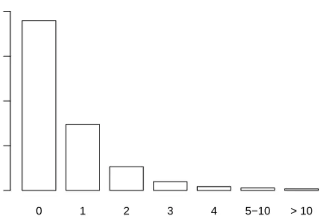
The most consistent solution to this problem would be to consider complete observations only, i.e. to remove all observations with one or more missing values. This, however, often leads to an immense loss of information. Moreover, this approach might bias the results of further analyses (Greenland and Finkle, 1995). For example, in the GENICA study (see Section 3), a study dedicated to the identification of genetic and gene-environment interactions associated with sporadic breast cancer, using complete observations would mean that data of just 63.3% of the women are considered (see Figure 1). Therefore, procedures are required that enable the replacement of missing values instead of removing them and the corresponding observations.
In the analysis of gene expression data, KNNimpute proposed by Troyanskayaet al.(2002) is a popular method to impute missing expression values based on weightedknearest neighbors (kNN; Fix and Hodges, 1951). Let’s assume that the expression value xij of gene i and
observation j is missing, and that Lk is a set comprising the k genes showing the smallest
Euclidean distance to geneiand having a value present for thejth sample. Using KNNimpute, xij is replaced by xij = X ℓ∈ Lk wiℓxℓj . X ℓ∈ Lk wiℓ, (1)
where the weightwiℓis given by the reciprocal of the Euclidean distance between the expression
values of geneiand geneℓ.
For an application of KNNimpute to protein expression data and a comparison of the Euclidean distance with other distance measures and of the weighted mean (1) with other estimates of average in the context of KNNimpute, see Jung et al.(2006).
However, KNNimpute cannot be employed for replacing missing genotypes, since SNPs are categorical variables. In this article, we therefore introduce an approach based on weighted k nearest neighbors enabling the imputation of missing categorical data. This procedure called KNNcatImpute is then compared to other imputation methods such as the tree-based procedure proposed by Dai et al. (2006) and the imputation approach of Random Forests (Breiman, 2001) in their applications to the SNP data from the GENICA study.
Contrary to other non ad hoc imputation methods that take the information in all variables into account when replacing missing values, KNNcatImpute is not restricted to “classical” as-sociation studies in which several ten to a few hundred SNPs are considered, but can also be applied to data from whole-genome studies. To exemplify this, we employ this approach to impute the missing genotypes in a subset of the SNP data from the HapMap study (The International HapMap Consortium, 2003) consisting of 262,264 SNPs and 90 persons. More-over, we compare KNNcatImpute with imputation methods that can also be used for replacing
missing values in such high-dimensional data.
This paper is organized as follows. In Section 2, KNNcatImpute is presented in detail, and it is shown how matrix algebra can be employed to determine all distances required by k nearest neighbors simultaneously. While in Section 3 this procedure is applied to the GENICA data set and compared with other approaches, Section 4 consists of the comparison of KNNcatImpute and other imputation procedures in their application to the subset of the HapMap data.
2
Imputation of missing genotypes based on
k
nearest
neighbors
2.1
Distance measures for categorical data
If k nearest neighbors are to be determined for categorical data, a distance measure has to be employed that can cope with this type of data. Such measures are typically based on an R×C contingency table in which the joint distribution of two variables, sayY andZ, with observation vectorsy andz, each of length n, is represented by the numbers
nrc= n
X
j=1
I(yj=r)I(zj=c) (2)
of observations showing therth level atY,r= 1, . . . , R, and thecth level atZ,c= 1, . . . , C. An example for such a distance measure is given by
dCont y,z=
q
1−Cont2 y,z
, (3)
where the corrected Pearson’s contingency coefficient Cont y,z = s min R, C min R, C −1 · χ2 χ2+n
is based on Pearson’sχ2-statistic
χ2 = R X r=1 C X c=1 (nrc−n˜rc)2 ˜ nrc = R X r=1 C X c=1 n2 rc ˜ nrc − n
for testing the null hypothesis that the two variables are independent by comparingnrc with
˜ nrc= 1 n C X c=1 nrc R X r=1 nrc, (4)
i.e. the numbers of observations expected under the null hypothesis.
In this article, we assume thatR=C, i.e. that all variables exhibit the same number of categories. In the case of SNPs,R= 3, where 1 denotes for the homozygous reference genotype (which is the form that typically shows up most often), 2 the heterozygous genotype, and 3 the homozygous variant.
Besides distances based on Pearson’sχ2-statistic for testing independence of two variables,
variables into account. A popular example is the distance dSMC y,z= 1−sSMC y,z= 1− 1 n R X r=1 nrr (5)
that is based on the (generalized) simple matching coefficientsSMC.
Another measure that also uses the total number of agreements/matches aR=
R
X
r=1
nrr,
but additionally takes into account the number of agreements that would have been found by chance, i.e.eR=Pr˜nrr, is the distance
dCohen y,z= 1−κC= 1−
aR−eR
n−eR
= n−aR n−eR
based on Cohen’s kappa κC (Cohen, 1960).
All these distance measures treat the SNPs as categorical variables, i.e. assume that the distance between the two homozygous genotypes is equal to the distance between each of the homozygous and the heterozygous genotype. A different idea is to take the number of base exchanges into account such that the distance between the homozygous genotypes (two base exchanges) is twice the distance between a homozygous and the heterozygous genotype (one base exchange). Using the abovementioned coding of the genotypes as numeric values, an appropriate measure for this idea is the scaled Manhattan distance
dMan y,z = 1 2n n X i=1 |yi−zi|. (6)
In Section 3.2 and Section 4.2, these four measures are compared in the application of KNNcatImpute to the SNPs from the GENICA and the HapMap study, respectively.
2.2
KNNcatImpute
After having computed the values of an appropriate distance measure dfor all pairs of SNPs, a missing genotypexij of SNPi and observationj is imputed by first identifying the set Lk
comprising the k SNPs showing the smallest distances to SNPi and having a value present for thejth observation. Then,xij is determined by weighted majority voting, i.e. by
xij= arg max r=1,...,R X ℓ∈Lk d−1 xℓ·,xi· I xℓj=r , (7)
wherexℓ· is a vector containing the genotypes of SNPℓfor all observations. Note that in (7) the normalization factorP
ℓ∈Lkd
−1(x
ℓ·,xi·) is omitted, since – contrary to (1) – the value of
xij is not affected by this constant. Ifd(xℓ·,xi·) = 0 for anyℓ∈ Lk, thenxij is replaced by
xℓj.
2.3
Simultaneous computation of contingency tables
Applying KNNcatImpute to a data set composed ofm variables andnobservations requires the calculation ofm(m−1)/2 distances. Since computing these values one-by-one can be very
time-consuming, we employ the vectorization and matrix computation functionalities of the statistical software R (R Development Core Team, 2007) to speed up the computation of the values of the distance measures based on contingency tables.
Suppose thatXis an m×n matrix in which each row represents one of themvariables, and each column corresponds to one of the nobservations. For a start, assume that none of the values are missing. IfX(r)denotes anm×nindicator matrix,r= 1, . . . , R, with elements
x(ijr)= 1, ifxij =r 0, ifxij 6=r(or xij is missing) ,
then the upper triangle of them×mmatrix
N(rc)=X(r)X(c)′ (8)
contains the numbers nrcfor allm(m−1)/2 pairs of variables, cf. (2), and the lower triangle
consists of the numbersncr of these pairs,r, c= 1, . . . , R. More precisely, the value of (2) for
the two SNPs represented by the ith and the ℓth row ofXis given by the (ith, ℓth) element ofN(rc). Analogously, ˜ N(rc)= 1 nX (r)1 n1′nX (c)′. (9)
is composed of the expected numbers ˜nrc and ˜ncr, cf. (4), where1ndenotes a vector of length
nconsisting only of ones.
Using (8), them×mdistance matrixDSMC containing the distancesdSMC, see (5), for all
m(m−1)/2 pairs of SNPs can be computed by
DSMC=1m,m− 1 n R X r=1 Nrr, (10)
where1m,mis anm×mmatrix consisting only of ones. Similarly, the distance matrixDCohen
can be computed by employing (8) and (9).
For the distance matrixDCont, anm×m matrixQcontaining all m(m−1)/2 values of
Pearson’sχ2-statistic needs to be determined by
Q= R X r=1 R X c=1 N(rc) ∗N(rc) ˜ N(rc) −n, (11)
where * and the fraction line denote elementwise matrix calculations.
Them×mdistance matrixDMancomposed of the values of the scaled Manhattan distance
(6) can also be determined by matrix computation. For this, note that ifyiandzi,i= 1, . . . , n,
are integers between 1 and R, then (6) can also be calculated by
dMan y,z= 1 2n R X r=1 R X c=1 c6=r |r−c| ·nrc
such thatDMan is given by
DMan= 1 2n R X r=1 R X c=1 c6=r |r−c| ·N(rc). (12)
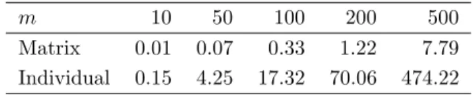
TABLE 1. Processing times (in seconds) of both the matrix algebra based and the individual calculation of the values of Pearson’s χ2
-statistic for all pairs ofm categorical variables, where each variable exhibitsr= 3 levels, and the number of observations isn= 1,000.
m 10 50 100 200 500
Matrix 0.01 0.07 0.33 1.22 7.79 Individual 0.15 4.25 17.32 70.06 474.22
If there are missing values inX, the matrix algebra based procedure will lead to incorrect distances for variables exhibiting missing values, since the number of observations showing no missing value at such a variable will differ from the total numbernof observations. To extend this approach to a matrixX containing missing values, it is therefore necessary to define an m×nmatrixXNA with elements
xNAij = 1, ifxij is not missing 0, ifxij is missing ,
and to replacenin (9)-(12) by the m×mmatrixN=XNA XNA′
.
Since the rowwise sums of X(r) in (9) only take individual but not pairwise missing
val-ues, i.e. missing values appearing in either of the two considered variables, into account, it additionally is necessary to replaceX(r)1
n byZ(r)=X(r) XNA
′
such that (9) becomes ˜
N(rc)=Z
(r) Z(c)′
N .
2.4
Comparison of processing times
To evaluate how much an implementation of the procedure based on matrix calculation in R accelerates the computation in comparison to an individual determination of the m(m−1)/2 values of Pearson’sχ2-statistic, both approaches are applied to several numbersmof variables. In Table 1, the resulting processing times on an AMD Athlon XP 3000+ machine with 1 GB of RAM are summarized. This table reveals that using the vectorization and matrix computation functionalities of R speeds up computation substantially, in particular if m is large. If, e.g., 500 variables are considered, then it takes just less than 8 seconds to obtain the 124,750 values of Pearson’sχ2-statistics when employing matrix computation, whereas an
individual calculation requires about 8 minutes.
3
Application to an Association Study
3.1
GENICA data set
The GENICA study is a case-control study carried out by the interdisciplinary study group onGeneENvironmentInteraction and breastCAncer in Germany (http://www.genica.de), a joint initiative of several German research institutes dedicated to the detection of genetic and environmental factors leading to a higher risk of developing sporadic breast cancer. The cases and controls of this age-matched and population-based study have been recruited in the
0 1 2 3 4 5−10 > 10 Missing Values Number of Women 0 200 400 600 800
FIGURE 1. Distribution of the numbers of missing values over the 1,234 observations from the GENICA study.
larger Bonn region, Germany, between 2000 and 2002. For more details, see Justenhovenet al.
(2004).
In this article, the focus is on a subset of the genotype data from the GENICA study. More precisely, data of 1,234 women (609 cases and 625 controls) and 39 SNPs belonging to the estrogen, the DNA repair, or the control of cell cycle pathway are available for the analysis.
Since a few of the women show many missing genotypes (see Figure 1), all 35 observations with more than three missing values are removed from the analysis leading to a total of 1,199 women (592 cases and 607 controls). The missing values of these women could, of course, also have been imputed. We, however, prefer to remove such observations – as long as their number is small – since observations with many replaced values may add large uncertainties to further analyses with, e.g., discrimination methods.
The remaining 1.3% missing values should be replaced by the imputation method that performs best in a comparison of already existing approaches for imputing categorical data with KNNcatImpute. But first we would like to investigate which parameter setting is best suited for an application of KNNcatImpute to the GENICA data set.
3.2
Comparison of parameter settings
Contrary to the discrimination approach of k Nearest Neighbors (see., e.g., Ripley, 1996) in which the k nearest observations are employed to predict the class of a new observation, Troyanskaya et al. (2002) borrow strength from a huge number of genes by imputing the missing values based on theknearest genes.
In the GENICA data set, however, the number of observations is much larger than the number of SNPs. To figure out which approach works best for the GENICA data, KNNcatIm-pute therefore is not only applied toXto identify theknearest SNPs, but also toX′to detect theknearest observations.
Moreover, it is examined which of the distance measures presented in Section 2.1 is most suitable in the analysis of the GENICA data set.
For these comparisons, only the genotypes of the 759 complete observations, i.e. women without missing values, are taken into account. Since in the GENICA data set 1.3% of the
0 10 20 30 40 50 0.34 0.38 0.42 0.46 Error Rate 0 10 20 30 40 50 0.34 0.38 0.42 0.46 0 10 20 30 40 50 0.34 0.38 0.42 0.46 0 10 20 30 40 50 0.34 0.38 0.42 0.46 0 10 20 30 40 50 0.34 0.38 0.42 0.46 Error Rate Nearest Neighbors 0 10 20 30 40 50 0.34 0.38 0.42 0.46 Nearest Neighbors 0 10 20 30 40 50 0.34 0.38 0.42 0.46 Nearest Neighbors 0 10 20 30 40 50 0.34 0.38 0.42 0.46 Nearest Neighbors
FIGURE 2. Mean fractions of falsely imputed values if dSMC (left-most panel), dCohen (second left-most panel), dCont (second right-most panel), or dMan (right-most panel) is employed in KN-NcatImpute to replace the 1% (upper panel) or 2% (lower panel) artificially generated missing values in the GENICA data set. The solid lines mark the error rates whenk nearest observations are used, and the dashed lines the error rates whenk nearest SNPs are considered.
genotypes are missing and the common rate of missing values in association studies is 5%-10% (Dai et al., 2006), we remove randomly 1%, 2% 5%, and 10% of the genotypes, respectively. Afterwards, the (artificial) missing values are replaced using the different settings of KN-NcatImpute, and the imputed values are compared with the real genotypes. This procedure is repeated 50 times.
In Figure 2, the mean fractions of falsely imputed genotypes for different values ofkand different settings of KNNcatImpute are displayed. (Since for all four cases, i.e. 1%, 2%, 5%, and 10% artificially removed values, the plots look similar, only the error rates for the imputations of the 1% and 2% missing values are presented.) This figure reveals that the distance dCont
based on the corrected Pearson’s contingency coefficient exhibits larger error rates than the three other measures when used in KNNcatImpute. The other three measures perform almost equally well when searching for the knearest observations, whereasdCohenshows larger error
rates than dSMC and dMan when considering thek nearest SNPs. For small values of k, k
nearest SNPs performs better thanknearest observations which might be due to the fact that in these cases mostly SNPs from the same gene are used to impute the missing genotypes (see also M¨ulleret al., 2005).
Therefore, the most suitable setting of KNNcatimpute for imputing the 1.3% missing genotypes in the GENICA data set seems to be an approach based onknearest observations withk≈50 and on one of the distance measuresdSMC,dCohen anddMan.
3.3
Comparison of imputation procedures
To determine how well KNNcatImpute performs in comparison to other imputation methods, three ad hoc approaches and two more sophisticated procedures are also applied to the data sets with the artificially generated missing values described in Section 3.2. In this comparison, we do not consider haplotype-based imputation methods (e.g., Dai et al., 2006), since we do not have haplotype information on the SNPs from the GENICA study.
In the three ad hoc approaches, the removed genotypes are imputed by
• the SNP-wise mode, i.e. typically the homozygous reference genotype,
• a random draw from the conditional distribution of the SNP given the case-control status.
The first more sophisticated method is based on Random Forests (Breiman, 2001). In this procedure, the missing values are initially replaced by the mode of the respective variable. Afterwards, Random Forests is applied to this data set, and the proximity, i.e. the fraction of trees containing two particular observations in the same terminal node, is computed for each pair of observations. The missing genotypes are then recalculated by weighted majority voting, where the votes resulting from the trees are weighted by the proximities. This procedure is repeated several times, and the values determined in the final iteration are the estimates for the missing genotypes.
The second approach proposed by Daiet al. (2006) is based on a combination of Gibbs sampling (see, e.g., Gelman et al., 2003) and CART (Breimanet al., 1984). Gibbs sampling is used to iteratively sample from the conditional distribution of the missing data of the jth observation given the values computed for the missing genotypes of the other observations in the previous steps of Gibbs sampling and the complete data of all observations, whereas CART is employed to model this full conditional distribution (for more details, see Daiet al., 2006).
For the comparison, the settings of KNNcatImpute leading to the best results in Section 3.2 are used, whereas the two more sophisticated methods are optimized by considering different values of their parameters. While in the CART based approach 1, 2, 5, 10 (recommended by Dai et al., 2006), 15 and 20 iterations are examined, the Random Forests based method is applied to the data sets using, on the one hand, one to six iterations, and on the other hand, 500, 1000 and 2000 trees with⌊√39⌋= 6, 3, 12 and 39 SNPs selected randomly from the 39 GENICA SNPs at each node (cf. Breiman, 2001).
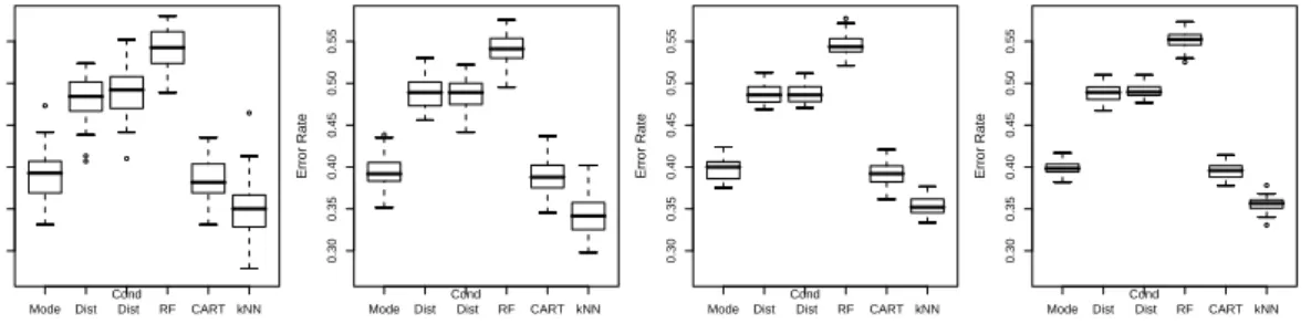
In Figure 3, the fractions of falsely imputed genotypes of the applications of these pro-cedures with optimized parameters are displayed. This figure reveals that KNNcatImpute leads to lower error rates than the approach of Dai et al. (2006) and the imputations based on the mode which in turn exhibit lower error rates than the other procedures. Therefore, KNNcatImpute seems to be best suited for the imputation of the missing values from the GENICA data set, and is therefore used to replace these genotypes.
Mode Dist Cond Dist RF CART kNN 0.30 0.35 0.40 0.45 0.50 0.55 Error Rate Mode Dist Cond Dist RF CART kNN 0.30 0.35 0.40 0.45 0.50 0.55 Error Rate Mode Dist Cond Dist RF CART kNN 0.30 0.35 0.40 0.45 0.50 0.55 Error Rate Mode Dist Cond Dist RF CART kNN 0.30 0.35 0.40 0.45 0.50 0.55 Error Rate
FIGURE 3. Boxplots of the fractions of falsely imputed genotypes when replacing the 1% (left-most panel), 2% (second left-most panel), 5% (second right-most panel), or 10% (right-most panel) missing values by the mode, by a draw from the SNP-wise distribution, by a draw from the conditional distri-bution of the SNP given the case-control status, by the Random Forests based method (5 Iterations, 500 trees with 6 SNPs at each node), by the CART-based procedure of Dai et al. (2006) with one
4
Application to Whole-Genome Data
4.1
HapMap data set
The International HapMap Project (http://www.hapmap.org; The International HapMap Consortium, 2003) is a collaboration of several scientific groups from different countries. In this project, millions of SNPs have been genotyped for each of 270 persons from four popula-tions, namely 45 Japanese from Tokyo, 45 Han Chinese from Beijing, 90 Yoruba in Ibadan, Nigeria, and 90 CEPH (Utah residents with ancestry from Northern and Western Europe).
About 500,000 of these SNPs have been measured using the Affymetrix GeneChip Mapping 500K Array Set composed of the Nsp and the Sty array. In this article, we focus on the geno-types of the 262,264 SNPs from the Nsp arrays that have been determined by the standard Affymetrix genotype calling algorithm BRLMM (Bayesian Robust Linear Models with Maha-lanobis distance; Affymetrix, 2006). These genotypes can be downloaded from http://www. affymetrix.com/support/technical/sample data/500k hapmap genotype data.affx.
Furthermore, we only consider the genotypes of the 45 Japanese and 45 Han Chinese, since all these individuals are unrelated, whereas each of the other two populations consists of 30 trios each of which is composed of data from a mother, a father and their child. For imputing missing genotypes in the latter two populations, it therefore might be more appropriate to take into account the relationship between the observations.
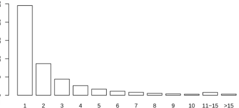
Since 45,793 of the 262,264 SNPs are monomorph, i.e. show only one genotype, and there-fore useless for discriminating the two populations, they are removed from the data set prior to the application of the imputation methods, although all procedures considered in this sec-tion can handle such SNPs. For 46,118 of the remaining 216,471 SNPs, at least one of the 90 genotypes is missing. In Figure 4, the distribution of the numbers of missing values for these 46,118 SNPs is displayed.
As a relatively small number of SNPs exhibits a large number of missing values, all SNPs exhibiting less than 90% non-missing values are removed leading to 44,733 SNPs with at least one missing genotypes. The remaining 0.49% missing values in this subset of the HapMap data set should again be replaced by the imputation method leading to the smallest numbers of falsely imputed values.
1 2 3 4 5 6 7 8 9 10 11−15 >15 Missing Values Number of SNPs / 1000 0 5 10 15 20 25
FIGURE 4. Distribution of the numbers of missing genotypes in the 46,118 SNPs from the HapMap data that show at least one missing value.
TABLE 2. Mean fractions of falsely imputed genotypes when applying KNNcatImpute with different distance measures and different numbers of nearest neighbors to the HapMap data sets in which either 1% or 2% of the values have been removed randomly.
k 1 3 5 7 dSMC 0.142 0.147 0.153 0.158 1% dCohen 0.148 0.153 0.156 0.159 Removed dCont 0.531 0.542 0.549 0.556 dMan 0.140 0.145 0.150 0.155 dSMC 0.143 0.148 0.154 0.159 2% dCohen 0.150 0.154 0.157 0.160 Removed dCont 0.364 0.374 0.382 0.389 dMan 0.142 0.146 0.151 0.156
4.2
Comparison of parameter settings
To figure out which of the distance measures and how many nearest neighbors should be used in KNNcatImpute to replace the missing values in the HapMap data set, 1% and 2% of the values of the 170,353 SNPs without missing genotype are removed randomly, and then imputed using KNNcatImpute with different parameter settings to compare the imputed values with the real genotypes. This procedure is repeated 20 times.
Contrary to the application of KNNcatImpute to the GENICA data set in which all SNPs/observations are considered in the search for theknearest SNPs/observations, we here “just” use the SNPs without missing values to identify theknearest neighbors of a SNP with missing values. Moreover, we restrict the search by considering the SNPs chromosomewise such that the missing genotypes of a particular SNP are imputed using only SNPs that come from the same chromosome as the considered SNP. The latter is not only time-saving, but also biologically meaningful, as only SNPs from the same chromosome are inherited together. In Table 2, the mean fractions of falsely imputed values are summarized for the different settings of KNNcatImpute. This table shows that while employing the corrected Pearson’s contingency coefficient works poorly also in the application to the HapMap data, the other three distance measures perform almost equally well, where the scaled Manhattan distance exhibits slightly lower error rates thandSMCwhich in turn leads to slightly less falsely imputed
genotypes thandCohen. For all distance measures, using one nearest neighbor in
KNNcatIm-pute performs best, whereas employing seven nearest neighbors leads to the largest error rates.
4.3
Comparison of imputation procedures
For comparison, the three ad hoc methods from Section 3.3 are also applied to the data sets with artificially generated missing genotypes. The imputation methods of Daiet al.(2006) and Breiman (2001), however, cannot be used to replace these missing values, as it is not feasible to apply these procedure to whole-genome data, even if the SNPs with missing genotypes are considered chromosomewise. This shows an advantage of KNNcatImpute: Contrary to other approaches that take not only the values of the variable whose missing values should
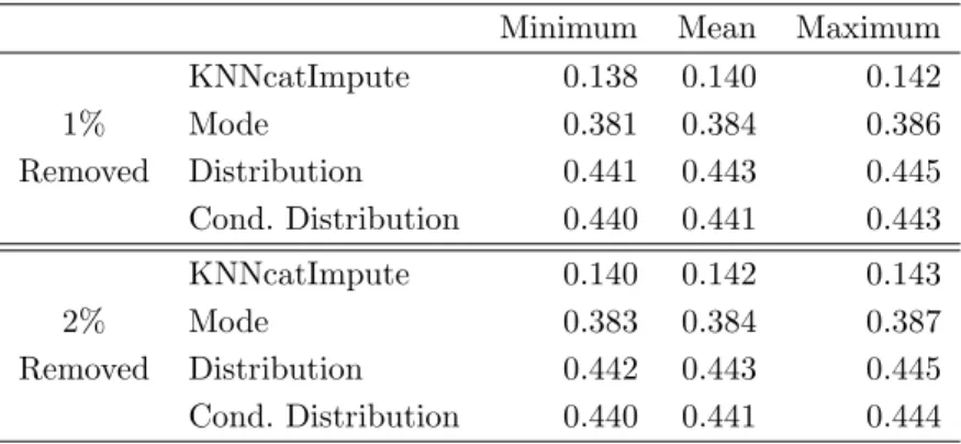
TABLE 3. Minimum, mean and maximum of the fractions of falsely imputed genotypes determined in applications of four imputation methods to the HapMap data sets in which either 1% or 2% of the values have been removed randomly.
Minimum Mean Maximum KNNcatImpute 0.138 0.140 0.142 1% Mode 0.381 0.384 0.386 Removed Distribution 0.441 0.443 0.445 Cond. Distribution 0.440 0.441 0.443 KNNcatImpute 0.140 0.142 0.143 2% Mode 0.383 0.384 0.387 Removed Distribution 0.442 0.443 0.445 Cond. Distribution 0.440 0.441 0.444
be replaced into account, but employ the information of all variables to impute these missing values, KNNcatImpute can be applied to whole-genome data.
Table 3 in which the fractions of falsely imputed genotypes of both the three ad hoc methods and KNNcatImpute usingdManandk= 1 nearest neighbor are displayed reveals that
KNNcatImpute exhibits substantially smaller error rates than the other imputation methods. We therefore replace the 93,927 missing genotypes in the subset of the HapMap data set described in Section 4.1 by applying KNNcatImpute to these data, which takes about 28 minutes on an AMD Athlon XP 3000+ with 1 GB of RAM.
5
Discussion
Missing genotypes are a common problem in association studies. Since many statistical meth-ods cannot handle missing values, they need to be removed or replaced prior to the actual analysis. In this article, we have presented a method based on weightedk nearest neighbors for imputing missing values in categorical data such as SNP data.
In a comparison with other imputation methods, this procedure called KNNcatImpute shows the lowest fractions of falsely imputed genotypes when applied to the SNP data from the GENICA study.
In our comparison, no haplotype-based imputation approach has been considered, since for the GENICA data set we do not have information on haplotypes, i.e. on blocks of SNPs that are inherited together and are therefore (highly) correlated. If such information is available, haplotype-based methods might improve the imputation of missing genotypes. However, KNN-catImpute is able to identify groups of highly correlated SNPs, and should therefore also work well in comparison to such approaches when haplotype information is available.
An advantage of KNNcatImpute over other imputation methods that also take not only the distribution of a particular SNP, but the information from all SNPs into account to impute the missing values of this SNP is that KNNcatImpute can be applied to data from whole-genome studies, whereas it is infeasible to use other non ad hoc imputation approaches such as the procedure based on Random Forests and the method of Dai et al. (2006) to replace missing
values in such high-dimensional data sets.
To exemplify this KNNcatImpute is applied to a subset of the SNP data from the HapMap project. In a comparison with other imputation methods that only consider the distribution of the SNP whose missing values should be replaced, KNNcatImpute shows the by far smallest fractions of falsely imputed genotypes.
As in the application of KNNcatImpute to the GENICA data set, employing the distance measures dSMC, dCohen and dMan that take the numbers of matches between the genotypes
or the alleles of two SNPs, respectively, into account lead to almost the same fractions of falsely imputed genotypes in the analysis of the HapMap data set, whereas the distancedCont
based on the corrected Pearson’s contingency coefficient, which is comparable to a correlation coefficient in the analysis of continuous data, performs poorly in the applications to both data sets.
Although KNNcatImpute has been developed in the context of SNP data, it is not restricted to such data, but can also be applied to other types of categorical data. However, in such an application all variables should show the same number of categories, and the meaning and the order of the categories should be the same for all variables so that distance measures such as dSMC anddCohen can be employed appropriately.
Acknowledgement
The financial support of the Deutsche Forschungsgemeinschaft (SFB 475, “Reduction of Com-plexity in Multivariate Data Structures”) is gratefully acknowledged. The authors would also like to thank Tina M¨uller for fruitful discussions on distance measures, Ingo Ruczinski for pro-viding the R function of the imputation method of Dai et al.(2006), and all partners within the GENICA network for their cooperation.
References
Affymetrix (2006). BRLMM: An improved genotype calling method for the GeneChip Human Mapping 500k array set. Technical report, Affymetrix , Santa Clara, CA.
Breiman, L. (2001). Random Forests. Mach. Learn.,45, 5–32.
Breiman, L., Friedman, J., Olshen, R., and Stone, C. (1984). Classification and regression trees. Wadsworth, Belmont, CA.
Cohen, J. (1960). A coefficient of agreement for nominal scales. Educ. Psychol. Meas., 20, 27–46.
Culverhouse, R., Suarez, B., Lin, J., and Reich, T. (2002). A perspective on epistasis: Limits of models displaying no main effect. Am. J. Hum. Genet.,70, 461–471.
Dai, J., Ruczinski, I., LeBlanc, M., and Kooperberg, C. (2006). Imputation methods to improve inference in SNP association studies. Genet. Epidemiol.,30, 690–702.
Fix, E. and Hodges, J. (1951). Discriminatory analysis – nonparametric discrimination: con-sistency properties. Technical report, USAF School of Aviation Medicine.
Garte, S. (2001). Metabolic susceptibility genes as cancer risk factors: Time for a reassessment?
Cancer Epidemiol. Biomarkers Prev.,10, 1233–1237.
Gelman, A., Carlin, J., Stern, H., and Rubin, D. (2003). Bayesian data analysis. Chapman & Hall, London, second edition.
Goodman, J., Mechanic, L., Luke, B., Ambs, S., Chanock, S., and Harris, C. (2006). Exploring SNP-SNP interactions and colon cancer risk using polymorphism interaction analysis. Int. J. Cancer, 118, 1790–1797.
Greenland, S. and Finkle, W. (1995). A critical look at methods for handling missing covariates in epidemiologic regression analysis. Am. J. Epidemiol.,142, 1255–1264.
Heidema, G., Boer, J., Nagelkerke, N., Mariman, E., van de A, D., and Feskens, E. (2006). The challenge for genetic epidemiologists: how to analyze large numbers of SNPs in relation to complex diseases. BioMed Genet.,7(23).
Hoh, J. and Ott, J. (2003). Mathematical multi-locus approaches to localizing complex human trait genes. Nat. Rev. Genet.,4, 701–709.
Jung, K., Gannoun, A., Sitek, B., Apostolov, O., Schramm, A., H.E., M., St¨uhler, K., and Urfer, W. (2006). Statistical evaluation of methods for the analysis of dynamic protein expression data from a tumor study. REVSTAT,4, 67–80.
Justenhoven, C., Hamann, U., Pesch, B., Harth, V., Rabstein, S., Baisch, C., Vollmert, C., Illig, T., Ko, Y., Br¨uning, T., and Brauch, H. (2004). ERCC2 genotypes and a corresponding haplotype are linked with breast cancer risk in a German population. Cancer Epidemiol. Biomarkers Prev., 13, 2059–2064.
Kooperberg, C. and Ruczinski, I. (2005). Identifying interacting SNPs using Monte Carlo logic regression. Genet. Epidemiol., 28, 157–170.
Lunetta, K., Hayward, L., Segal, J., and van Eerdewegh, P. (2004). Screening large-scale association study data: exploiting interactions using Random Forests.BMC Genet.,10(32). Marchini, J., Donnely, P., and Cardon, R. (2005). Genome-wide strategies for detecting
multiple loci that influence complex diseases. Nat. Genet.,37, 413–416.
M¨uller, T., Selinski, S., and Ickstadt, K. (2005). Cluster analysis: a comparison of different similarity measures for SNP data. Technical report, SFB 475, Department of Statistics, Dortmund University of Technology.
Nunkesser, R., Bernholt, T., Schwender, H., Ickstadt, K., and Wegener, I. (2007). Detect-ing high-order interactions of sDetect-ingle nucleotide polymorphisms usDetect-ing genetic programmDetect-ing.
Bioinformatics. doi: 10.1993/bioinformatics/btm522.
R Development Core Team (2007).R: A Language and Environment for Statistical Computing. R Foundation for Statistical Computing, Vienna, Austria. ISBN 3-900051-07-0.
Ripley, B. (1996). Pattern recognition and neural networks. Cambridge University Press, Cambridge.
Ritchie, M., Hahn, L., Roodi, N., Bailey, L., Dupont, W., Parl, F., and Moore, J. (2001). Multifactor-dimensionality reduction reveals high-order interactions among estrogen-metabolism genes in sporadic breast cancer. Am. J. Hum. Genet.,69, 138–147. Ruczinski, I., Kooperberg, C., and LeBlanc, M. (2003). Logic regression. J. Comput. Graph.
Stat.,12, 475–511.
Schwender, H. and Ickstadt, K. (2007). Identification of SNP interactions using logic regres-sion. Biostat. doi:10.1093/biostatistics/kxm024.
The International HapMap Consortium (2003). The International HapMap Project. Nature,
426, 789–796.
Troyanskaya, O., Cantor, M., Sherlock, G., Brown, P., Hastie, T., Tibshirani, R., Botstein, D., and Altman, R. (2002). Missing value estimation methods for DNA microarrays. Bioin-formatics, 17, 520–525.