Owner time and cost contingency estimation for building construction projects in Egypt

(1)

American University in Cairo American University in Cairo

AUC Knowledge Fountain

Theses and Dissertations

6-1-2017

Owner time and cost contingency estimation for building

construction projects in Egypt

Seif El-Din Nawar

Follow this and additional works at: https://fount.aucegypt.edu/etds

Recommended Citation Recommended Citation

APA Citation

Nawar, S. (2017).Owner time and cost contingency estimation for building construction projects in Egypt [Master’s thesis, the American University in Cairo]. AUC Knowledge Fountain.

https://fount.aucegypt.edu/etds/667

MLA Citation

Nawar, Seif El-Din. Owner time and cost contingency estimation for building construction projects in Egypt. 2017. American University in Cairo, Master's thesis. AUC Knowledge Fountain.

https://fount.aucegypt.edu/etds/667

This Thesis is brought to you for free and open access by AUC Knowledge Fountain. It has been accepted for inclusion in Theses and Dissertations by an authorized administrator of AUC Knowledge Fountain. For more information, please contact [email protected].

(2)

School of Sciences and Engineering

OWNER TIME AND COST CONTINGENCY ESTIMATION FOR

BUILDING CONSTRUCTION PROJECTS IN EGYPT

A thesis submitted to the School of Sciences and Engineering

in partial fulfillment of the requirements for the degree of

Master of Science in Construction Engineering

To

Department of Construction Engineering

By

Seif El-Din Essam Mostafa Nawar

B. Sc. In Construction Engineering, 2013

Under the Supervision of

Dr. Ossama Hosny

Dr. Khaled Nassar

Professor Associate Professor Construction Engineering Construction Engineering The American University in Cairo, Egypt The American University in Cairo, Egypt

(3)

ii

Acknowledgment

In this section, I would like to seize the opportunity to make acknowledgment to all who have supported and mentored me to achieve my current academic and professional standing. I would like to start by expressing sincere gratitude and appreciation to my thesis advisors, Dr. Ossama Hosny and Dr. Khaled Nassar, for their efforts, continuous support, guidance and mentorship throughout my research. They truly served as great mentors, and always availed the time to follow up on my work and offer advice. Not to mention, they served as the instructors of many courses I have attended during my academic journey at AUC.

Sincere appreciation goes to my family members, father and mother, who have always provided encouragement and all kind of support throughout this journey. They truly served as a main source of determination and motivation throughout my life.

Many thanks goes to all the Construction Engineering department faculty in the American University in Cairo who tutored me and served as a great valuable instructors for all the courses I have attended during undergraduate and graduate programs. They have been role models and true inspiration, which made real impact in my life and many others.

I would like to thank Dr. Hatem El-Behairy for his guidance in using fuzzy logic. Thanks also goes to Engineer Kareem Zahran for his time to guide and help me finish my research. Moreover, I would like to thank my close friends who provided moral support and encouragement.

(4)

iii

Abstract

Time and cost overruns are an integral part of the construction projects. Both have several associated negative consequences to the project owners. Setting the right time and cost contingency is a major contributing factor to the success of the project as it should minimize/prevent budget and time overruns. Project managers usually tend to allocate project time and cost contingency subjectively based on their previous experience and may not capture all projects specific factors that impact the contingency estimation. The competency of the project manager plays an important role in this case in determining the contingency percentage. The contingency estimation for a given project can hugely vary from one project manager to another. This research presents a fuzzy logic-based model that allows owners predict the project time and cost contingency reliably and accurately in Egypt. The most important factors affecting time and cost contingency have been identified and are defined as input variables for the model. The effect of these factors on the time and cost contingency, the output variables, have been determined and incorporated into the model via fuzzy rules. On the basis of the known effects of these factors, a fuzzy logic model is developed to automate the prediction process using MS Excel software. Several scenarios of the model are developed and subjected to initial testing using 10 actual projects data. Based on the initial testing, the best model was subjected to tuning in order to achieve the optimum model results in terms of accuracy and validity. Finally, the model is tested by applying it on new five actual construction projects which were not used in the initial testing nor tuning. The model results were found to be acceptable having an average validity percent of 84% and 81% for time and cost contingency, respectively. The proposed model allows the owners to [1] understand the effect of the project different factors on the contingency values, which in turn represent the degree of risk involved and accordingly, allows the owner to take necessary measures at the preconstruction stage to reduce the risks, [2] minimize the cost and time overrun through setting the right amount of contingency, [3] avoid tie up of excessive funds for the project, which can be used in others projects or activities, and [4] have higher confidence during the decision making process of whether to proceed or not to proceed with the project.

(5)

iv

List of Figures

Figure 1 Research Methodology... 4

Figure 2 Project Total Time Allowance (Project Time Contingency) (Barraza, 2011) ... 11

Figure 3 Activity Time Allowance (ATA) (Barraza, 2011) ... 11

Figure 4 Neural Connection Methodology (Yahia et al., 2011) ... 20

Figure 5 Reliability Buffer at Merging Point (Park and Pena-Mora, 2004) ... 22

Figure 6 Budgeting Owner Contingency Methodology (Gunhan and Arditi, 2007) ... 26

Figure 7 General Proposed Framework for Cost Contingency Estimation (Polat and Bingol, 2013) ... 29

Figure 8 Membership Function for Input Variables (Polat and Bingol, 2013) ... 30

Figure 9 Membership function for the Output variables (Polat and Bingol, 2013) ... 30

Figure 10 ERA worksheet for a Construction project at the conceptual design stage (Mak and Picken, 2000) ... 34

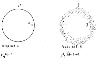
Figure 11 Difference between Crisp Set and Fuzzy Set (Nguyen, 1985) ... 36

Figure 12 Age membership (Rojas, 1996) ... 37

Figure 13 Background of Questionnaire Respondents ... 51

Figure 14 Years of Experience of Questionnaire Respondents ... 51

Figure 15 General framwork of the proposed contingency model ... 55

Figure 16 Respondents Years of Experience ... 57

Figure 17 Respondents Experience Background ... 57

Figure 18 Numerical Scale for the possible scenarios of the factors ... 59

Figure 19 A snapshot of the model interface part where the user inputs the rating for the 11 factors ... 70

Figure 20 Output of Rules Calculation and Resultant Contingency ... 70

Figure 21 Membership Function of the Input Variable “Scope Definition” ... 75

Figure 22 Cost Contingency Membership Function Sample ... 75

Figure 23 Time Contingency Membership Function Sample ... 75

Figure 25 User Interface to define the input variables, ranges and unit ... 93

Figure 24 User Interface to Define Membership Functions ... 93

Figure 26 User Interface to input the rating of a factors for a given project to calculate the contingency ... 94

(8)

vii

List of Tables

Table 1 Factors affecting Time Contingency (Mohamed et al, 2009) ... 15

Table 2 Typical Pair-Wise Comparison Matrix for Different Factors (Mohamed et al, 2009) ... 15

Table 3 Factors Affecting Time Contingency based on Literature (Yahia et al, 2011) ... 18

Table 4 Most Important Factors Affecting Time Contingency (Yahia et al, 2011) ... 19

Table 5 Results of the ANN model (Yahia et al, 2011) ... 20

Table 6 Three MRAM models and their significance levels (Polat and Bingol, 2013) ... 31

Table 7 Regression Parameters and their significance levels (Polat and Bingol, 2013) ... 31

Table 8 Relationship between Risk Allowance and Risk Category (Mak and Piken, 2000) ... 33

Table 9 Comparison between ERA and non-ERA projects (Mak and Picken, 2000) ... 35

Table 10 Fuzzy logic applications in the Construction Industry ... 38

Table 11 Factors Affecting Time and Cost Contingency based on Literature Review ... 45

Table 12 Rating of factors obtained from Second Round of Questionnaire ... 52

Table 13 Top 11 factors identified via the questionnaire ... 53

Table 14 List of Questionnaire Respondents ... 56

Table 15 Cost and Time Contingency Output Rating Scale ... 63

Table 16 Input Variables Acronyms ... 65

Table 17 Effect of factors on the Owner Time and Cost Contingency ... 68

Table 18 Contingency Rating Scores ... 69

Table 19 Projects Data Obtained from Questionnaire ... 71

Table 20 Actual Projects Data obtained from Questionnaire ... 72

Table 21 Model Scenarios Developed for Initial Testing ... 73

Table 22 Cost Contingency Results Comparison of Different Scenarios ... 73

Table 23 Time Contingency Results Comparison of Different Scenarios ... 74

Table 24 Model Results in Prediction of Time Contingency and Performance Measurement ... 76

Table 25 Model Results in Predicting Cost Contingency and Performance Evaluation ... 77

Table 26 Actual Projects Data Used for Validation ... 78

Table 27 Actual Projects Data Obtained from Questionnaire for Validation ... 78

Table 28 Model Outputs Results in Predicting Time Contingency ... 79

(9)

1

1. Introduction

1.1 Background

The construction industry plays an important role as a major driving force for other sectors’ growth (Samarghandi et al., 2016). The construction sector constitutes a significant percentage of the overall gross domestic product (GDP) of any country. In year 2005, it constituted 3.3% of Malaysia’s GDP and employed circa 600,000 workers (Sambasivan and Soon, 2007). Meanwhile, in the United Arab Emirates (UAE), it constitutes 14% of the GDP (Ravisankar et al., 2014). The construction sector is one of the most dynamic and growing sectors in Egypt (Shibani, 2015). According to the Egyptian Ministry of Planning, it constituted mainly 4.8% of the total GDP in the year 2013. Ahmed (2003) (as cited by Abd El-Razek et al., 2008) states that, since 1981, the construction industry was allocated approximately 45% of the funds for the national development plans in Egypt since it is one of the most active sectors that affects the Egyptian economy to a great extent.

Completion of a construction project within the time, cost and quality targets determines whether a project is successful or not. The project manager endeavors to complete the project in its allotted time and cost frames (Rosenfeld, 2014). Various unexpected negative effects occurs in line with failure to achieve the project targets (Sambasivan and Soon, 2007). Time and cost overruns occur in most construction projects worldwide and have become an integral part of the construction industry (Rosenfeld, 2014). Delay and cost overrun of construction projects is a global phenomenon and rarely is a construction project completed following the original estimates whether time or/and cost (Assaf and Al-Hejji, 2006; Marzouk et al., 2008; Sambasivan and Soon, 2007; Wanjari and Dobariya, 2016). This can be attributed to the fact that construction projects are vulnerable to many factors, which impose significant effects on them whether positive or negative. Assaf and Al-Hejji (2006) stated that these factors usually result from many sources which may include, but not limited to environmental conditions, political conditions, market conditions, resources availability, and involvement and performance of parties. Some of those factors are predictable and controllable while others are not. Hence, uncertainty does exist in all construction projects, which in turn impose risks on achieving project targets, namely time, cost and quality.

(10)

2

1.2 Delay in Construction Projects

Delays in construction simply exists when the project completion date exceeds the specified completion date stipulated in the contract agreement or the date which the parties previously agreed on to complete the project (Assaf and Al-Hejji, 2006). In other words, delay in construction projects exists when there is a deviation between the actual completion date and the planned completion date. Delay is harmful to both parties of the contract of a construction project, which are mainly the employer and the contractor. From the contractor point of view, it is a loss of profit due to delay damages, higher overhead costs, and maybe higher labor and material costs in the long term (Assaf and Al-Hejji, 2006; Marzouk et al., 2008). From the owner point of view, it is a loss of revenues because by the time the project is completed and operation starts, it should be generating revenues, which will be delayed. (Assaf and Al-Hejji 2006; Marzouk et al., 2008). Accordingly, time is equivalent to money in construction projects.

1.3 Cost Overruns in Construction Projects

A common problem in the construction industry is cost overruns (Nassar et al., 2005). Cost overrun occurs when the project costs exceed its allocated budget (Wanjari and Dobariya, 2016). It is also defined as a budget overrun or increase in cost due to unexpected costs incurred. This may result from several causes which include, but not limited to, lack of project control, inefficient planning and design deficiencies. Other reasons include budget error, and additional scope not captured prior to budget sign-off (Al-Hazim and Salem, 2015). Exceeding the budget requires additional funding by the owner. In some cases, additional funding may not be available which may cause risk of project suspension. In large multinational organizations, additional funding requires approvals that take long time, efforts and needs extensive justifications by the project managers.

1.4 Problem Statement

A growing demand exists for advanced construction systems and models capable of solving complex problems in line with the complexities and rapid advancement of the industry. Duran (2006) (as cited in Gunduz et al., 2014) states that many projects are not completed on time; as a result, a very bad reputation is attributed to the construction industry regarding time adherence and usually project managers encounter the blame. Majid (2006) and Mahamid et al. (2012) (as cited in Gunduz et al, 2014) stated that the most common unfavorable outcomes are the loss of productivity, loss of revenues, cost overrun, and disputes. Exceeding budget is a

(11)

3 dilemma as well for project managers and have several unfavorable consequences. Therefore, it is crucial that contingency should be determined accurately during the planning stage in order to enable the owner’s project manager avoid exceeding project completion dates and budgets with their unfavorable consequences. However, it should be noted also that having an excessive unneeded contingency will tie up funds from being used in another potential projects or activities. To specify a time and budget contingency, project managers usually rely on traditional methods which are based on subjectivity, gut feeling, experience and intuition and do not rely on a mathematical method to support them in their decision (Gunhan and Arditi, 2007; Touran, 2003; Mohamed et al., 2009). This leads to an underestimated or overestimated contingency value.

Literature shows that cost contingency has been studied extensively more than time contingency had. However, the majority of the previous studies are from the contractors’ point of view to allow them incorporate a cost contingency in their bid prices while very few are from the owner’s point of view that would enable them set their contingency. In addition, few attempts has been made earlier to predict cost contingency in Egypt. Also, literature shows few research about time contingency prediction when compared to cost contingency. Similar to cost contingency, available studies are made though specifically for contractors to enable them predict the contingency and assign it to their baseline construction schedules, but very few attempts were made to predict the owner time contingency that enables them set a high level time contingency in the project master schedule. Despite the cost and schedule of construction projects are interrelated, cost and time contingency models are usually separated and independently applied (Bakhshi & Touran, 2014). Thus, this research will propose a reliable method that will enable the prediction of both time and cost contingency from the owner’s point of view in an attempt to help owners and decision makers understand the effect of setting the project parameters on the contingency amount and allows them to be confident towards the agreed project cost and time.

1.5 Objective and Scope

The aim of this research is to [1] Identify factors affecting time and cost contingency from the owner side in Egypt, [2] Develop a reliable mathematical model to predict the owner time and cost contingency for their building construction projects, [3] Allow owners’ decision makers to set the project contingency amounts accurately and avoid overestimation or underestimation, and [4] increase owners confidence towards the agreed project time and cost.

(12)

4

1.6 Research Methodology

Figure 1 shows a flow chart that demonstrates the methodology followed in this research to achieve its objectives.

Figure 1 Research Methodology

First of all, a literature review shall be conducted to explore the available research addressing contingency prediction. Focus will be on the techniques that are used, and the summary and conclusions of the studies. A literature summary is then developed highlighting the

1

• Conduct literature review to explore available research addressing contingency estimation

2 • Identify factors that affect time and cost contingency from literature review

3

• Design and distribute a questionnare to determine the most relevant and significant factors affecting owner time and cost contigency in Egypt

4 • Develop a mathematical model to predict the owner time and cost contingency

5

• Design and distribute a questionnaire to construction professionals to obtain real projects data to be used for model verification and validation

6 • Conduct initial testing and tuning for the model

7 • Validate the model using real projects data

(13)

5 gaps or areas that can have further research. The second step is to identify a long list of factors affecting owner time and cost contingency from literature. This long list is then subjected to elimination of factors that are considered irrelevant and/or redundant, which will result in having a shortlist. The third step is designing and disseminating a questionnaire to determine the most significant factors affecting owner time and cost contingency in Egypt using Delphi technique. The most significant factors are the ones that shall be used in the research and shall be part of the mathematical model, which is to be developed in the fourth step. Once the mathematical model is developed, a second questionnaire shall be designed and distributed in order to obtain actual projects data to be used for both verification and validation. Initial testing and tuning will be applied to the model first using real projects data to ensure the best model is developed. After choosing the best model, different real projects data will be used to validate the model and finally, conclusions, recommendation and limitations of the research are stated.

1.7 Thesis Structure

The following are the chapters of this research. All chapters serve each other in order to form a comprehensive thesis.

A- Chapter 1: Introduction

This chapter provides an introduction about the construction delays and cost overruns, the reasons they are unfavorable to project parties and the degree of their prevalence. It also contains the problem statement, objectives, scope, methodology and finally thesis organization.

B- Chapter 2: Literature Review

This chapter presents information and facts about delays and cost overuns in the construction industry. It also presents previous research done to predict construction projects’ time and cost contingency including the methods used. Finally, the gap found in the literature is presented and discussed.

C- Chapter 3: Research Methodology

This chapter aims to introduce the methods used throughout this research in addition to the inputs and outputs of each step. It outlines the factors affecting owner time and cost contingency identified. It presents the model development strategy and techniques that are used. It also shows

(14)

6 the quesionnaire design developed to gather real projects data to be used in initial testing, tuning and validation processes.

D- Chapter 4: Model Development, Initial Testing and Tuning

This chapter presents the process of the model development including design approach, different design scenarios, variables, rules, assumptions and finally results of initial testing and tuning based on real case studies.

E- Chapter 5: Case Studies Applications

This chapter contains the results of the model developed on real case studies for validation purposes through comparing the model prediction results with actual data.

F- Chapter 6: Conclusion, Limitations and Recommendations

This chapter concludes the research stating the findings, limitation of the research and finally, recommendations for future work and development.

(15)

7

2. Literature Review

2.1 Occurrence of time and cost overrun in construction projects

It has been reported by several researchers that delays are common in the construction sector worldwide. The average time overrun in construction projects in Saudi Arabia was between 10% and 30% and only 30% of the projects finished within the planned date of completion (Assaf and Al-Hejji, 2006). Ajanlekoko (1987) (as cited by Sambasivan and Soon, 2007) stated that performance of construction projects in Nigeria was poor in terms of time. Odeyinka and Yusif (1997) (as cited by Sambasivan and Soon, 2007) found that out of ten projects surveyed in Nigeria, only three projects finished within planned time. In India, out of 951 surveyed projects, 474 projects were found to be behind schedule and not completed within the stipulated time in the contract (Doloi et al., 2012). In Hong Kong, Chan and Kumaraswamy (1995) (as cited by Lo et al., 2006) observed that 75% of private sector construction and 60% of government related construction experienced delays and were not completed on time. According to a study conducted by World Bank in 2007, between 1999 and 2005, many projects completed worldwide with a time overrun varying between 50% and 80% (Ravisankar et al., 2014). “Modernizing Construction” report, prepared in the United Kingdom (UK) by the National Audit Office, stated that only 30% of the government department and agencies’ projects were delivered on time (Ravisankar et al., 2014). Accordingly, many studies have been conducted to identify causes and rankings of delays (AlSehaimi et al., 2013).

Several research have been made in Egypt to identify and rank causes of delay, which implies prevalence of delay and its wide occurrence. Ezeldin and Abdel-Ghany (2013) reported that time overruns are a repetitive phenomenon in the Middle East and in Egyptian construction industry. Literature shows that delays in construction industry have been investigated and discussed in numerous manners. Mainly, the following are the most common topics that were covered by different studies addressing delay in construction industry.

 Causes of delay and its ranking according to project type (Al-Hazim and Salem, 2015)

 Causes of delay and its ranking according to country (Shibani, 2015; Lo et al., 2006; Abd

El-Razek et al., 2008; Aziz, 2013)

 Delay Analysis (Sutrisna et al., 2016)

(16)

8

 Delays mitigation (Abdul-Rahman et al., 2006)

 Prediction of future delay while construction is on-going (Li et al., 2006)

 Prediction of Time claims (Hosny et al., 2015)

 Estimating the probability of delay of construction projects (Gunduz et al., 2014)

 Estimating time contingency (Pawan and Lorterapong, 2016); however, literature shows

limited coverage

One of the major contributing factors to reduce the occurrence of delays in construction projects and meet the time schedule is allocating accurate time contingency. Time contingency should be well studied to be accounted for while scheduling for construction projects.

It has been reported by several researchers that cost overruns are common as well in the construction sector worldwide. Several construction projects exceed initially set cost limits due to in ability to account for uncertainties and factors that result in cost overruns and exceeding the project budget (Ahiaga-Dagbui and Smith, 2014). In road construction projects in Australia, Baccarini (2004) (as cited by Jr. et al, 2010) reported that the average cost overrun was 9.92% and the average contingency was 5.24%. Wanjari (2016) reported that out of 410 projects that were reviewed in India, only 43% were completed on budget and 57% experienced cost overrun. Flyvbjerg et al. (2003) (as cited by Rosenfeld, 2014) analyzed 258 transportation-infrastructure projects gathered from five continents and found that the average budget escalation was 28%. Ahiaga-Dagbui and Smith (2014) reported that 50% of the projects in UK exceeded their budget according to a government-commissioned report in 1998. In the US, the General Accounting office issued a similar report indicating that 77% of the projects overspent budget (Ahiaga-Dagbui and Smith, 2014). Hartley and Okamoto (1997) (as cited by Nassar et al., 2005) states that cost overrun of 33% on average occurs in construction projects. According to the Florida Department of Transportation, the construction cost overruns for 102 completed projects were found to be 9.5% above the initial approved budget (Nassar et al., 2005). Previous studies have been conducted in Egypt to identify factors affecting cost overrun (Aziz, 2013; Shibani, 2015) in addition to studies that attempted to predict cost overrun (El-Kholy, 2015). This demonstrates the prevalence of the cost overruns in Egypt. Several research has been made to study cost overruns in construction projects. In order to reduce the occurrence of exceeding projects budget in construction projects, cost contingency should be well studied to be accounted for while setting budget in the project planning stage.

(17)

9

2.2 Factors affecting time and cost contingency

Previous research attempted to identify the factors that directly affect the cost and time contingency, as well as factors that affect time and cost overruns (Gunhan and Arditi, 2007; Polat and Bingol, 2013; Hosny et al., 2015; Marzouk and El-Rasas, 2014; Idrus et al., 2011; Jr. et al., 2010; Mohamed et al., 2009; Yahia et al., 2011; Marzouk et al., 2008; Abd El-Razek et al.,2008; Shibani, 2015; El-Kholy, 2015; Kholif et al., 2013; El-Touny et al., 2014; Aziz et al., 2013). Long lists of factors are usually prepared and identified from literature by researchers. In some case, the next step is the identification of the most significant factors using surveys and ranking them using an index such as the Relative Importance Index (RII), Importance Index (II), Severity Index (SI) and Frequency Index (FI). By exploring factors identified from several authors, it was noticed that many factors are the same and identified by several authors, but mainly vary in the ranking. This could be due to location of the research, the type of projects, the size of projects, and whether it is from the owner side, consultant side or the contractor side.

2.3 Prediction of time contingency in construction projects

As the construction industry is full of uncertainties and unexpected events that happen during execution, projects’ parties encounter difficulties while planning for their projects prior to the construction phase. Generally, several factors should be taken into consideration to be accounted for during the planning phases. Among the main factors are the duration, the cost, the resources required for the project, the method statements to be used, the contract type, etc. Touran (2003) and Abou Rizk (2005) stated (as cited by Mohamed et al., 2009) that some factors are ambiguous and couldn’t be determined accurately and they are always taken as guesstimates based on previous experience and projects’ conditions. These are mainly the cost and time contingency, which are very important as construction projects always tend to deviate from the original plan (Mohamed et al., 2009).

If the schedule of the project does not account for such uncertainties, the completion date will not be achieved and the project will be considered unsuccessful. Given the construction projects are unique in nature and every project is not similar to another, the project schedule should incorporate time contingency and project specific uncertainties to accommodate any changes without affecting the overall project duration negatively (Mohamed et al., 2009). Another main reason for necessity of proper estimating time contingency is that delays have negative impacts on the project quality and budget (Mohamed et al., 2009). Time contingency is considered

(18)

10 to be a major factor for a successful construction project (Mohamed et al., 2009). Project Management Institute (PMI, 2000) defined contingency as “the amount of money or time needed above the estimate to reduce the risk of overruns of project objectives to an acceptable level to the organization”. Time contingency is usually expressed as percentage of the original total project duration (Touran, 2003).

Previous research has been conducted to predict time contingency. Khamooshi and Cioffi (2013) (as cited by Pawan and Lorterapong, 2016) stated that CPM is the common method for scheduling and planning of construction projects; however, it has been criticized that it doesn’t account for uncertainty inherent in construction projects. As a result, probabilistic based methods, such as Monte Carlo Simulation and Programme Evaluation and Review techniques (PERT) have been introduced as more objective approaches to overcome this limitation, but they require historical project data in order to be able to generate the probability density functions (Pawan and Lorterapong, 2016; Barraza, 2011). In order to obtain historical data for these techniques, these require extensive impractical efforts and time. Due to the merge event bias, PERT may provide very optimistic project schedules in some cases (Barraza, 2011).

Barraza (2011) developed a framework that determines the total project time contingency and allocates it among the individual activities by the stochastic allocation of project allowance (SAPA) method, which is mainly based on Monte Carlo simulation. Total time allowance (TTA) is the difference between the project planned duration (PPD) and the project target duration (PTD). Probabilistic method approach is used to calculate these estimates using simulation. Simulation results in different possible activity durations from the corresponding probability distributions and accordingly different possible project durations. Typically, the possible project durations follows a normal distribution curve regardless of the distribution of the activities durations. Project duration estimates can be selected from different project duration outcomes due to different risk levels, which can be defined as the probability that the selected

project duration is exceeded. Accordingly, depending on the acceptable risk level (∝𝑝𝑑) by the

project manager, the PPD can be determined. For example, the chosen PPD value can be the

duration with 15% chance of being exceeded, which corresponds to the 85th_{duration percentile.}

To estimate PTD, instead of using their expected or most likely values, median durations are considered where they are obtained from the simulation results easily. Having calculated both

(19)

11 PTD and PPD, the TTA now can be obtained as the difference between them and be allocated to the project activities as shown in Figure 2.

Figure 2 Project Total Time Allowance (Project Time Contingency) (Barraza, 2011)

Following the determination of the TTA, the total allowance should be allocated to the project activities. The method proposed in this research in order to estimate the PPD for each

activity is that a maximum allowed duration percentile (𝐷𝑃𝑖) with same risk level (∝𝑡) for all

project activities should be selected. Therefore, the PPD is the summation of the (𝐷𝑃𝑖). The

activity target duration (𝑇𝐷𝑖) shall be set as the median duration. Accordingly, the planned activity

time allowance (𝐴𝑇𝐴𝑖) can be calculated as the difference between both as per Equation (1) and

as demonstrated in Figure (3). Accordingly, it is concluded that TTA is the summation of the ATAs of the activities on the critical path.

𝐴𝑇𝐴𝑖 = 𝐷𝑃𝑖− 𝑇𝐷𝑖 Eq. 1

Figure 3 Activity Time Allowance (ATA) (Barraza, 2011)

This framework attempted to estimate the time contingency on the project level and its allocation on the activity level. Among the advantages of the SAPA method is that a fair distribution of the project time contingency is determined by predicting the maximum allowed

(20)

12 duration for all project activities at the same percentile level. In other words, larger planned durations will obtained for higher risk activities. The proposed method considers only predictable risks that may affect the performance of the activity; however, doesn’t consider the unforeseen conditions at the project level and the author recommended that these should be considered in a separate general time contingency prediction (Barraza, 2011).

On another note, critique has been made to probabilistic scheduling methods revealing their inability in considering non-random uncertainty (Pawan and Lorterapong, 2016). Construction projects are unique and accordingly, each project has its specific risks that may not apply to others, so the historical data incorporated in these methods may not be relevant to the future projects. In the current practice, experienced professionals tend to subjectively estimate durations incorporating contingencies; however, these subjective estimates may not be accurate and are subject to flaws and errors depending on the experience of estimators (Barraza, 2011). Therefore, advanced models are recommended to be developed that would enable reliable prediction of time contingency considering vagueness and imprecision encountered during project scheduling. Critical Chain management was also introduced to account for variations in activity durations where two types of buffers are used, the feeding buffer and the project buffer. Certain heuristic approaches are used in order to determine the size of these buffers, which are mainly the root square error method and the cut and the paste method. However, It has been proven that both methods are incapable to create robust schedules (Pawan and Lorterapong, 2016).

Given literature showed that fuzzy set theory has been successful and captured the interest of researchers through the last three decades in modeling uncertainty, Pawan and Lorterapong (2016) used fuzzy set theory in order to overcome the vagueness and imprecision when predicting time contingency. They developed a model to take into account the risks impact on construction activity duration estimation and develop a scheduling procedure that shows the effectiveness of risk response planning to reduce time contingency. Therefore, fuzzy logic was employed in order to model the time contingency needed for the execution of the activities affected by the risks. Not only does the model enable modeling of single risk impact, but also multiple risks impacts. Their framework is as follows.

a- Risk Identification: Identifying all risks that may impact to the project activities obtaining

(21)

13

b- Risk Analysis: Risks are analyzed by determining the probability of occurrence (∝𝑖) and

the impact of the each of the risks associated to a particular activity. The impact is the resultant extension of time in case the risk occurred to the activity, which is estimated usually by experienced construction professionals subjectively and based on imprecise linguistic expressions such as around 6 to 8 days or circa 10 days. In this research, the resultant extension of time should the risk occurred is called “Fuzzy Time Extensions” (FTE).

c- Impact Quantification: FTE determined previously are based that the risk factor will

definitely occur. Accordingly, adjusted FTE (AFTE) is obtained when there is lack of

confidence with the possibility of 𝑅𝑖 to occur. AFTE can be calculated using Equation (2)

Eq. 2

Where AFTE = Adjusted Fuzzy Time Extension; FTE = Fuzzy Time Extension;

∝𝑖 = the probability of occurrence;

d- Fuzzy Activity Time Contingency Calculation: if the activity is exposed to one risk factor,

then the time contingency needed is the AFTE. If the activity is exposed to multiple risk, then the time contingency is the combined AFTE of all risks. The maximum impact is taken assuming all risks are independent. As a result, the total activity duration, which is the fuzzy activity duration incorporating the risk (RFAD) may be calculated.

e- Development of Risk Incorporated Schedules: The fuzzy project schedule is determined

using the RFAD.

f- Risk Response Planning: after the schedule is developed using RFAD, the schedule

duration should be compared with the contract duration ensuring that contractual milestones are achieved and met. To be able to compare both values being considered, an agreement index (AI) is developed noting its value ranges from 0 to 1 where 0 is no agreement and 1 is full agreement. Based on the organization’s risk tendency, a guideline shall be set for AI values. If the AI value is below predetermined value, then immediate risk responses are required through identifying the associated activities that is resulting in the disagreement and low AI value. If the AI value is above predetermined value, then no action is required.

(22)

14 Moreover, Pawan and Lorterapong (2016) developed a framework involving fuzzy set theory that enables the integration of risk management into the project schedule by identifying risks associated with the project specific activities and accounting for it rather than setting a time contingency on high level basis or at the project level. The benefits of the fuzzy set theory is that it allows the modeling of the vagueness, imprecision and subjectivity usually inherent with the construction project schedules and as a result, it yields a robust project schedule. This framework is designed specifically for contractors’ use when developing their detailed construction baseline schedules, but doesn’t serve owners of construction projects when developing their master schedules at the planning stage before issuance of the project tender.

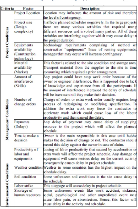
Mohamed et al. (2009) developed a model to estimate the time contingency for construction projects. The model involved the use of the Analytic Hierarchy Processes (AHP) where it depended on the factors that affect time contingency and their impact, which are identified through a survey and the literature. Table 1 shows the factors that have been chosen and included in the survey. The factors were categorized into project, environmental, and management conditions and the importance of each factor has been determined from the survey respondents.

(23)

15

Table 1 Factors affecting Time Contingency (Mohamed et al, 2009)

AHP has been chosen in this research to assess the weights of the factors affecting time contingency through pair-wise comparison matrices, which have important characteristics as shown in Table 2. At the intersection of each criterion and itself, the elements are all set to one.

(24)

16

The weight of the factors have determined through the Equation (3) 𝑤𝑥 is the weight of

the factor, n is the pair-wise comparison matrix dimension and 𝑎𝑖𝑗 is the matrix element for i row

and j column. The time contingency has been developed using Equation (4) where 𝐶𝐷 is the time

contingency, 𝑤𝑖 is the weight factor, 𝑠𝑖 is the score for each factor in a specific project and 𝑝𝑖 is

the factor’s probability of occurrence.

Eq. 3

Eq. 4

Moreover, the model implementation have been according to the following steps:

a. Calculating the relative weight of each major category

b. Calculating the sub-factors’ weights relative to the weight of its category

c. Calculating the 13 factors’ scores to determine the most effective to the contingency

value towards the least ineffective

d. Calculating the 13 factors’ probability of occurrence

e. Multiplying the probability of each factor by the weight by the effectiveness score

f. Obtaining the summation of the multiplication which represents the overall time

contingency of the project

The results of the study concluded that 36.78% of the original project duration should be allocated as time contingency to the project due to the effect of the contingency factors. AHP, however, considers each factor on its own and provides no correlation between the factors, which is not very representative for construction projects nature. The verification of the model was verified based on obtaining the average delay of seven projects and comparing it with the average contingency obtained from the survey results. Therefore, the model is not project specific since each project is unique and an average contingency is not accurate to be applied on all projects similarly.

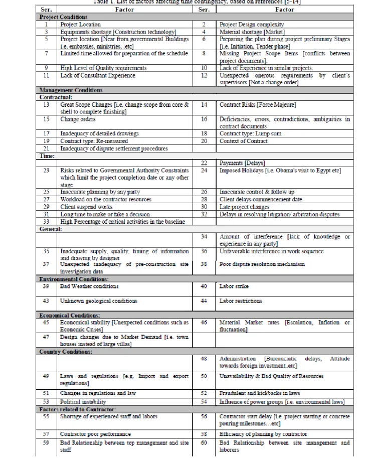
Yahia et al. (2011) developed an Artificial Neural Network (ANN) model to predict the time contingency in Egypt. They performed data collection to identify the factors that affects the

(25)

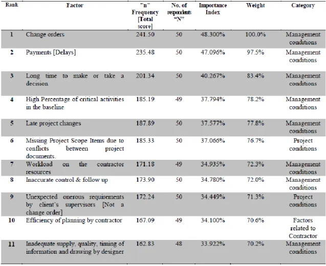
17 time contingency in Egypt. Table 3 lists all factors that have been identified through the literature. In order to identify the most important factors that would be considered in the model, the factors were ranked by construction market experts. The respondents had to insert scores for the factors. Scores were for the degree of impact of each factor and its probability of occurrence. Both scores then are multiplied by each other to get the time contingency effect. Yahia et al. (2011) used the importance index method to determine the level of importance of each factor by using the Equation (5).

Importance Index = ∑ [aX] x 100/10 Eq. 5

Where a = constant expressing the weighting ranges from 1 to 10 having 10 as the most important and 1 as the least important;

X = is the ratio between the frequency of the respondents (n) and the total number of respondents to each factor (N).

All factors having an important index above 70% were considered to be among the most important factors affecting the time contingency in the construction market. Table 4 contains the most important factors after analyzing the survey results. As ANN model requires historical data for training and testing purposes, data gathering for 54 building construction projects executed by Class A contractors were gathered through sessions with experts.

(26)

18

(27)

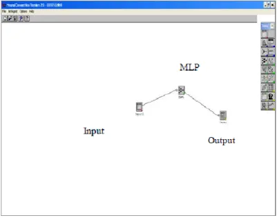
19 The most important factors listed in Table 4 were set as input nodes of the ANN model which the user should input his project specific parameters. Additionally, the user should input an additional factor, which is the project duration. In this research, back-Propagation (BP) learning algorithm, a multilayer feed-forward neural network architecture, has been used. Figure (4) shows the neural connection methodology. The error calculated at the network output is propagated through the layers of neurons to adjust the weights that would lead to the correct outputs. The BP works on minimizing the root mean square (RMS) error to link the input to the output mapping correctly. RMS is calculated using Equation (6). The model is trained when the RMS is minimized to an acceptable extent.

Eq. 6

(28)

20

Where 𝑂𝑖 = Sample Actual Output

𝑃𝑖 = The output predicted

N = No. of samples to be evaluated in training stage

The output node of the model was set as the time contingency in days, the input node contains the factors, while the MLP is the Multi-Layer Perceptron.

Figure 4 Neural Connection Methodology (Yahia et al., 2011)

For the model training, Forty Nine projects were used. After completion of training, the model was tested using the remaining five projects to determine the reliability and accuracy of its results. Table 5 shows the results of the testing. Yahia et al. (2011) found that the average time contingency for Egyptian Construction Projects was 28% and that the model predicted a reliable and acceptable time contingency with an absolute variance that ranged from 0% to 7.5%.

Table 5 Results of the ANN model (Yahia et al, 2011)

This research however is dependent on factors that are hardly known at the planning stage of the project or the pre-contract stage. This model mainly serves contractors to assist them in predicting time contingency in their detailed construction schedules, but not targeted for the

(29)

21 owners of the projects when developing their master programme. In order for the owner to determine the contingency, it should be based on information that is available and known at this early stage. The factors used in this model are known only while the construction is on-going. An example of these factors are: the no. of changes initiated in the last 25% of the project actual duration, number of Request for Information (RFIs) and Average of delay in each payment in days. Another limitation for using ANN to predict time contingency is that it has to be based on historical cases, which should be correct and accurate in order to train and teach the model predict the results reliably.

Another research done to predict contingency reliably was done by Park and Pena-Mora (2004), who criticized the usage of traditional time contingency buffering to guarantee activity or project completion time. They stated that this type of buffering results in an unnecessary resource idle time and often fails to protect the performance of the project schedule. Among the limitations of assigning a contingency buffers traditionally at the end of activities, site team usually tend to consume the contingency buffer as part of the original activity duration and hence, it is not a contingency anymore. The result is that the time contingency added results in schedule expansion. Sterman (as cited by Park and Pena-Mora, 2004) found that work productivity decreases when people know they have more time than the original time allowance to complete an activity as people tend to defer the work to the last minute. Also, Balard and Howel (1995) stated that (as cited in Park and Pena-Mora, 2004) sizing buffers is usually based on individual experience and assigned uniformly rather than considering activities characteristics. Accordingly, Park and Pena-Mora (2004) introduced “Reliability buffering” to address this issue. Reliability buffering is based on simulation and aims to result in a robust construction plan that takes into account uncertainties of individual activities and protects the schedule against them. Simulation of the model is used to determine the effectiveness of the reliability buffering. The methodology of reliability buffering is that it resizes, relocates and re-characterizes the contingency buffer and if no contingency buffer is available, a new buffer is introduced. Dynamic updates take place as well to the size and location of reliability buffers while the construction is on-going in order to account for any deviations in the schedule from the original estimates. To overcome the challenges of the traditional contingency buffering, Park and Pena-Mora tackled the limitations through introducing changes.

(30)

22 Starting with buffering logistics, they suggested to take-off the contingency buffers from being placed at the end of activity and assigning them in the front of the successor activity. This enables enough time to discover and rectify any problems from the preceding activity without affecting the successor activity duration. This will enable the option of dealing with ill-defined tasks issue that require time to define. Taking off contingency buffers from the end of the activities will lead to schedule pressure and to overcome the last-minute syndrome. Also, relocating buffers to the beginning of the activity duration, losses at the merging point of a schedule network are reduced. Figure (5) shows an example for the relocation of an activity buffer to the successor of the next activity.

Figure 5 Reliability Buffer at Merging Point (Park and Pena-Mora, 2004)

As for buffer sizing, it should be long enough to maintain the reliability of the successor activities; however, overestimated buffer time will lead to unproductive idle time. There are three main determinants for the buffer size, which are the following.

- Production type, which is mainly the activity work progress pattern.

- Sensitivity, which is the degree of activity sensitivity to changes made externally or

internally.

- Reliability, which is the degree of robustness against uncertainties and generic work

quality.

Initial planned buffers needs to be dynamically updated to be able to control schedule deviations from the original plan. When using static buffer, if the predecessor activity is delayed, it will push the successor activity and delay its planned start. However, when using dynamic buffering, if the predecessor activity is delayed, the impact can be minimized on the successor activity by updating dynamically the size and the location of the buffer based on the current project progress, actual information obtained resulting for the actual performance and the remaining construction performance forecast. If the predecessor activity finished earlier than

(31)

23 planned, dynamic buffering approach will seize the opportunity of schedule advance. Therefore, the following are the necessary steps needed to implement reliability buffering.

1- Taking off and pooling time buffers for the project activities

2- Adjusting the size of the contingency buffers or determining a new buffer considering the

project activity characteristics and control policies

3- Allocating the new buffers on the beginning of the successor activities

4- Characterization of the buffers as an available time that can be used to ramp up resources

for a successor activity and solving the problems of the predecessor activity that will impact the successor activity’s progress.

5- All remaining contingencies to be used as a pool buffer for the project

6- During Construction through measuring actual performance and having performance

forecast, enable dynamic update of the size, and location of buffers to meet the actual situation.

In conclusion, based on Park and Pena-Mora research findings, reliability buffering can result in robust construction schedule against uncertainties and shorten the project duration with no additional costs through appropriately pooled, resized, re-characterized and relocated buffer. Reliability buffering effectiveness is examined by simulation of a dynamic project model, which integrates the network scheduling approach with the simulation approach.

In addition to the limitations mentioned for previous research, there has been limited research to predict the owner time contingency that should be incorporated in the master schedule of the project, which is usually reported to the organization top management. The construction contingency is usually determined by the contractor in his detailed baseline schedule; however, the owner time contingency is usually added in the master schedule in order to account for any project delays due to uncertainties and unforeseen conditions.

2.4 Prediction of cost contingency in construction projects

Gunhan and Arditi (2007) states that there are many factors that makes forecasting accurate owner’s budget very difficult. Funding issues, design control, management of schedules and costs, performance of parties involved in the construction, inherent uncertainity, and complexity of the project are contributing factors that affect budget determination. Accordingly, project managers include contingency funds within the budget to account and cover those

(32)

24 uncertainites and ambiguites. Setting up the right contingency contributes to completing the project successfully.

Mills (2001) (as cited by Idrus et al., 2011) reported that traditionally many project managers determine cost contingency as 10% on the project estimated cost. Baccarini (as cited by Idrus et al., 2011) commented that this method is conventional and not easy to defend and justify.

Although high contingency ensures the design and construction will finish smoothly due to availability of sufficient funds; however, there are several drawbacks (Gunhan and Arditi, 2007). Among the major drawbacks is the tie up of funds that can be used in other activities and projects (Bakhshi and Touran, 2014). Another drawback is that large contingency sometimes can be questioned by the firm management and proper justification has to be available to defend the allocated contingency. On the other hand, underestimated contingency funds impose a risk of going over budget, which is not acceptable as well and implies lack of project planning and control, etc. Cost overruns are prevalent as demonstrated in section 2.2. Furthermore, cost estimates at the projects planning stages play important role and ranks among the highest in terms of priority (Ahiaga-Dagbui and Smith, 2014). Cost-benefit analysis, build or not-to-build decision by owner, future performances benchmark and guidance in selection of potential delivery partners are among the roles and benefits of cost estimates (Ahiaga-Dagbui and Smith, 2014). Knowing that contingency is part of the cost estimate, it has a direct impact on the end decision taken.

It is very important to understand types of cost contingency that are part of the project budget, the purpose of each, and the party in control. Contract terms as well are vital to understand and interpret correctly to enable proper and effective contract administration and reduce disputes. Gunahn and Arditi (2007) stated there are three types of contingency in construction, which are the following.

a- Designer Contingency: it is allowed in the preliminary budget for any potential cost

increases during the design development phase or generally, the pre-construction phase. By the time the construction starts, the design contingency could be absorbed by any modifications in the design. In case there are elements in the design not fully complete, this contingency should serve to cover for those items later on. In an ideal situation, when the construction starts, the design contingency should be eliminated as its role should have been completed ideally assuming the design is fully complete.

(33)

25

b- Contractor Contingency: It is allowed in the construction budget for any cost increases

during the construction phase. Cost increase may occur due to any construction unforeseen conditions, schedule related issues due to overtime works to accelerate progress, changes in market conditions, which may affect material and labor prices. This contingency is controlled by the main contractor and its accurate prediction is very important for the contractor success, which in turn will give him the capability to recover delays through overtime and additional shifts and will assist to reach the time target as well.

c- Owner Contingency: It is allowed in the budget and controlled by the owner. Its purpose

is to cover for any missing scope and requirements that was not captured early and included in the contract scope during the tender stage. Generally, it covers for change orders, changing the standards/specifications of work, different site conditions when the nature of work encountered during construction is different than what’s stated in the contract documents, Design errors, etc. It is vital for the owner to predict his contingency accurately that will enable him to cover additional expenses and complete the project on budget.

Gunhan and Arditi (2007) stated the most common methodology to predict any type of contingency is by previous experience and taking subjective figures. The most common method is to consider a percentage of the estimated contract value and add it as the contingency (Touran, 2003; Jr. et al., 2010). Following interviews with 12 contractors, respondents reported that none of them had any mathematical tools or any formalized techniques to evaluate and estimate contingency (Jr. et al., 2010). Some experts identified fixed cost contingency percentages for projects according to types of works. For example, experts estimated the contingency to be 15% of the original cost and duration for underground construction activities and tunneling activities, while 7.5% for the remaining project activities (Touran, 2003). The problem with this method is that it is deterministic and based on experience and subjectivity and does not consider all project-on-hand specific factors and conditions. Also, it does not quantify the contingency estimate degree of confidence. Therefore, there exists a need for a technique that predict cost contingency reliably on certain basis rather than subjectively.

Gunhan and Arditi (2007) developed a framework demonstrated in Figure (6) to determine the owner contingency budgeting, which is based on the following steps.

(34)

26

1- Obtaining and analyzing historical projects data and records

2- Line items’ identification that consume contingency funds

3- Setting and implementing necessary measures accordingly at the preconstruction stage

to minimize the likelihood of occurrence of these line items

4- Based on this information, estimate contingency funds

This framework enables the owner to determine contingency funds confidently and minimize contingency, so to avoid tie up of unnecessary value of funds while it can be used in other activities or projects.

Figure 6 Budgeting Owner Contingency Methodology (Gunhan and Arditi, 2007)

Gunahn and Arditi (2007) proposed the following items to be studied thoroughly by owners for the line items during the preconstruction phase because they impact the budget of the project directly:

1- Evaluation of existing site conditions must occur. Each site is unique and has specific

(35)

27 Accordingly, if these specifics are not accounted for in the project estimate during the preconstruction phase and design phase, this will surely impact the project cost.

2- The project schedule constraints should be early identified and accounted for the project

pricing and estimation. Schedule should reflect expected scenario as much as possible, an accurate start date and all details as available. Late site handover or limited access to works have impact on the project budget.

3- Experienced engineer has to conduct a comprehensive detailed review of design

drawings, specifications and construction documents is essential prior to the tender issuance. The quality of the tender documents reflects the constructability of a project. The ease in which a project can be built and the quality of the constructions documents determines the constructability level of the project. Arditi et al. (as cited by Gunahn and Arditi, 2007) concluded in a study that ambiguous, faulty or defective construction documents, incomplete design and conflicts between construction documents are major factors that affect the construability of the project and in turn affect cost and time contingency.

4- Poorly defined project scope will lead to owner changes due to missed scope and

additional items needed to complete the project. Changes initiated by the owner will require extra work and efforts by the contractor and in turn additional costs. Scope definition and control is the second highest causes of the cost overruns as stated in the Construction Industry Institute (1986).

If these factors are managed effectively during the preconstruction stage and the pre-tender issuance, most probably this will reduce the contingency usage for the line items identified and will prevent the need for a large contingency, which ties up funds that can be used in other projects. The limitation of this technique is its significant dependency on the previous project data availability, accuracy and relevance. Data availability could be challenging in some markets especially if the owner was not involved in a good amount of previous projects. Also, despite reference is made to historical project data to determine contingencies of line items, the decision is still made manually based on human witness of previous records and their analysis, which can be time consuming.

Hammad et al. (2016) proposed a solution of estimating and managing cost contingency throughout the project using a probabilistic method. Since this research is about contingency

(36)

28 estimation, only the estimation section will be covered from Hammad et al. research. A probability distribution function using Monte Carlo Simulation (MCS) is assigned to each project activity and selecting an appropriate confidence interval followed by summation of all the resultant contingencies of the activities on the critical path, which yields the overall project cost contingency. The use of MCS allows activities with high costs and uncertainties receive higher contingency with respect to others. Hammad et al. criticized the traditional method of determining the contingency subjectively as a percentage of the total project cost based on previous experience and intuition and did a case study to demonstrate the benefit of their proposed method over the traditional method. The results showed the probabilistic method yielded a more accurate contingency. The proposed method calculated a contingency of 4.2% and the traditional method yielded 7.2%, while the actual contingency used in the project was 3.2%. Accordingly, they highlighted that the overestimation of contingency could be the cause for losing a tender. This research focused on the known unknowns, or predictable factors and was specifically designed for the contractors use. In addition, they claimed that among the main benefits of this framework is simplicity, and does not require the project manager to have the knowledge of the advanced tools and methods. In a construction project, complex and time consuming models will not be used by industry professionals; accordingly, they have little value as stated by Hammad et al. (2016).

Polat and Bingol (2013) did a research to compare the performance of fuzzy logic and multiple regression analysis (MRA) in estimating cost contingency. This research provided contractors with a tool to estimate their contingency amounts to be included in their bids for international construction projects. Fuzzy logic is qualitative methodology rather than quantitative capable to represent uncertain, vague and incomplete information as it leans on rational and systematic critical thinking (Polat and Bingol, 2013). Construction projects are full of uncertainties due to several predictable and unpredictable factors. On the other hand, MRA is quantitative method with uncertain numerical data availability. The methodology used in the research was as follows.

1- Identifying factors affecting cost contingency from literature and categorizing them by risk

groups as shown in Figure (7).

2- Developing a framework of the estimation model is shown in Figure (7).

The cost contingency value (CC) is modeled as shown in Equation (7) as a function of the major

(37)

29

magnitudes (𝑅𝑀𝑗𝑖) in group 𝒾. The relation between both is expressed in Equation (8) where

n is the number of the risk factors in major risk group 𝒾.

Eq. 7

Eq. 8

Where MR is the average risk magnitude for a group of risk factors RM is the risk magnitude of a single factor

Figure 7 General Proposed Framework for Cost Contingency Estimation (Polat and Bingol, 2013)

3- Preparing a questionnaire to be distributed to experienced construction professionals to

obtain previous projects data. The questionnaire consisted of two parts. The first part aimed

to rate the magnitude of the factors (𝑅𝑀𝑗𝑖) linguistically on a scale consisting of low, medium

and high. The second part aimed to let the questionnaire’s respondents state the actual contingency percentage of the contract value (CC).

4- Development of fuzzy logic model and three stepwise MRA model

5- Setting performance evaluation criteria to evaluate the performance of the models. The Root

Mean Square Error (RMSE), Mean absolute percentage error (MAPE), coefficient of determination (R²), and coefficient of correlation (R) have been chosen in this research. After calculation of these criteria, the model with the highest R and R² and lowest RMSE and MAPE is the best.

6- Comparison of the results obtained from both models.

Starting by the fuzzy logic model, six input variables have been defined along with six membership functions in addition to one output variable with one membership function. The

input variables are the major risk groups (𝑀𝑅𝑖) while the output variable is the cost contingency

(38)

30 experienced construction professionals. The agreed membership functions for the input variables and the output variable are shown in Figures (8) and (9). Input variables have been assigned on a numerical scale between 1 and 3 while the cost contingency has been assigned on a numerical scale of 5% to 10% as shown on the x-axis. The y-axis however denotes the degree of membership. Low, medium and high linguistic terms have been used for representing the input and output variables. The authors stated that the triangular distribution was found to be appropriate for the input variables while trapezoidal distribution was appropriate for the output variable.

Figure 8 Membership Function for Input Variables (Polat and Bingol, 2013)

Figure 9 Membership function for the Output variables (Polat and Bingol, 2013)

87 if-then rules have been specified based on expert judgement where the conjunctive system of rules was chosen for rules aggregation. For the fuzzy inference system, Mamdani’s system was chosen in this research as it has been widely accepted based on literature. The fuzzy sets in Mamdani are used as a rule consequent. The fuzzy sets must have defined rules input by the user.