A N I N V E S T I G AT I O N O F FA C T O R S I N F L U E N C I N G
A L G O R I T H M S E L E C T I O N F O R H I G H D I M E N S I O N A L
C O N T I N U O U S O P T I M I S AT I O N P R O B L E M S
k e v i n
g r a h a m
Doctor of Philosophy
Institute of Computing Science and Mathematics
University of Stirling
D E C L A R AT I O N
I, Kevin Graham, hereby declare that all material in this thesis is my own original work except where reference has been given to other authors. The work presented here has not been submitted for the award or partial award of any other degree at the University of Stirling nor any other institute.
Stirling, November2019
A B S T R A C T
The problem of algorithm selection is of great importance to the optimisation community, with a number of publications present in the Body-of-Knowledge. This importance stems from the consequences of the No-Free-Lunch Theorem which states that there cannot exist a single algorithm capable of solving all possible problems. However, despite this importance, the algorithm selection problem has of yet failed to gain widespread attention . In particular, little to no work in this area has been carried out with a focus on large-scale optimisation; a field quickly gaining momentum in line with advancements and influence of big data processing. As such, it is not as yet clear as to what factors, if any, influence the selection of algorithms for very high-dimensional problems (> 1000) - and it is entirely possible that algorithms that may not work well in lower dimensions may in fact work well in much higher dimensional spaces and vice-versa. This work therefore aims to begin addressing this knowledge gap by investigating some of these influencing factors for some common metaheuristic variants.
To this end, typical parameters native to several metaheuristic algorithms are firstly tuned using the state-of-the-art automatic parameter tuner, SMAC. Tuning produces separate parameter configurations of each metaheuristic for each of a set of continuous benchmark functions; specifically, for every algorithm-function pairing, configurations are found for each dimensionality of the function from a geometrically increasing scale (from2to1500 dimen-sions). The nature of this tuning is therefore highly computationally expensive necessitating the use of SMAC. Using these sets of parameter configurations, a vast amount of performance data relating to the large-scale optimisation of our benchmark suite by each metaheuristic was subsequently generated.
From the generated data and its analysis, several behaviours presented by the meta-heuristics as applied to large-scale optimisation have been identified and discussed. Further, this thesis provides a concise review of the relevant literature for the consumption of other researchers looking to progress in this area in addition to the large volume of data produced, relevant to the large-scale optimisation of our benchmark suite by the applied set of common metaheuristics.
All work presented in this thesis was funded by EPSRC grant: EP/J017515/1through the DAASE project1
.
A C K N O W L E D G M E N T S
“Let not your mind run on what you lack as much as on what you already have” –Marcus Aurelius
“Why do we fall, Bruce? So we can learn to pick ourselves up” –Thomas Wayne (Batman Begins2005)
I am dedicating this thesis to my loving wife Tracy, my sons Carson and Callan and my dad Michael Graham.
My dad sadly passed away from an asbestos related disease at the beginning of my2nd year - a particularly difficult time for family and myself. Of all the occasions when things got tough during the course of my studies, one of the things that kept me going was his pride that I had gotten to where I was; not through luck or innate ability, but like he did his whole life - through hard work and dedication. Being a family-centric man, I still believe that hard work on its own could not have brought me to this point, but the love and support from my dad and my family throughout my life. We all miss his presence, humour and love but his memory will live on through his wife - my mum, sons and grandchildren for years to come.
My PhD years were not all filled with grief however, I married my wife Tracy and 3 years later we had our first son, Carson Michael Graham. I simply would not be here writing this now if not for the unconditional love and support Tracy has shown me over the years -extending far beyond PhD studies. Whenever I needed to vent, talk things over or was in dire need of mental support I could always count on her to be there for me - even when I needed to be ‘rescued’ from Nottingham University when I fell ill with severe appendicitis. I really could not have done any of this were it not for her.
I make no secret of the fact about how many times - and how close I came - to throwing in the towel. The illogical side of my psyche had me convinced that the PhD was ‘cursed’ -I had lost multiple supervisors (through work opportunities), family members, had several failed/abandoned projects, suffered severe illness and was getting nowhere fast despite my efforts. That’s until my son Carson was born, and then my son Callan Thomas Graham just short of2years later. Every day since then I vowed that I would show them how to not give
up, to keep fighting through obstacles in your way in order to become the best version of yourself and that getting knocked down only teaches us how to get back up - I didn’t want their first lesson in life to be to stop moving forward.
And so my sons, this is for you, your mummy and your grandad - Always remember that you are braver than you believe, stronger than you seem, smarter than you think and more loved than you’ll ever know.
Finally, I would like to thank my current supervisors Prof. Leslie Smith, Dr. Alexander (Sandy) Brownlee and Dr. David Cairns for all their help and support over the last two years -without whom I could not have reached this point. Also, I’d like to give thanks to a former supervisor - Dr John Woodward, who never gave up trying to organise me, even up to the day he took up his new appointment. Also, I’d like to thank my fellow PhD students for all the years of interesting discussion and laughter. In particular, I’d like to thank Jason Adair (now Dr. Adair) for all the help and support (both personally and work-based), chats and putting up with my long venting sessions on the not-so-rare occasion - and of whom will always be considered as a friend. Of course, I cannot forget my mum who has always shown me love and support throughout my life and who taught ME that getting knocked down only teaches us how to get back up.
L I S T O F P U B L I C AT I O N S
[42] Kevin Graham, Jerry Swan, and Simon Martin. The Blackboard Pattern for Metaheur-istics.In Proceedings of the Companion Publication of the2015Annual Conference on Genetic and Evolutionary Computation, pages1265-1267,2015.
[41] Kevin Graham and Leslie Smith. Comparing Hyper-heuristics with Blackboard Systems. Proceedings of the Genetic and Evolutionary Computation Conference Companion, pages1141-1145, 2017.
The publications listed here are related to previous research directions no longer being followed and are therefore not relevant to this thesis.
C O N T E N T S
i i n t r o d u c t i o n 1
1 i n t r o d u c t i o n t o t h e t h e s i s 2
1.1 Introduction . . . 2
1.2 Structure of the Thesis . . . 3
ii b a c k g r o u n d & l i t e r at u r e r e v i e w 5 2 c h a p t e r 2: o p t i m i s at i o n 6 2.1 Introduction . . . 6
2.2 General Optimisation . . . 7
2.2.1 Terminology . . . 7
2.2.2 A Formal Definition of an Optimisation Problem . . . 9
2.2.3 Problem Difficulty . . . 9
2.3 Classical Optimisation Methods . . . 11
2.3.1 Strong Methods . . . 12
2.3.2 Weak Methods . . . 16
2.4 Metaheuristic Optimisation . . . 17
2.4.1 What is a Metaheuristic? . . . 17
2.4.2 Exploration vs. Exploitation in Metaheuristics . . . 19
2.4.3 Problems Addressed by Metaheuristics . . . 20
2.4.4 Categorisations of Metaheuristics . . . 20
2.4.5 General Concepts . . . 22
2.5 Large-Scale Global Optimisation . . . 31
2.5.1 Cooperative Co-Evolutionary Algorithm . . . 34
3 c h a p t e r 3: c o n t i n u o u s o p t i m i s at i o n b e n c h m a r k f u n c t i o n s 42 3.1 Introduction . . . 42
3.2 What Makes a Function Difficult to Optimise . . . 42
3.3 Constructing a Custom Function Suite Versus Using Existing Benchmark Func-tion Suites . . . 46
3.4 Functions . . . 48
3.4.1 Summary of Functions . . . 49 4 c h a p t e r 4: m e ta h e u r i s t i c a p p r oa c h e s u s e d i n t h i s t h e s i s 50
4.1 Introduction . . . 50
4.1.1 Exposing Algorithm Parameters . . . 51
4.1.2 Solution Representation . . . 52
4.1.3 Neighbourhood Function . . . 52
4.2 Hill Climbing Algorithms . . . 54
4.2.1 Common Variations . . . 55
4.2.2 Global Optimisation with Hill Climbing . . . 58
4.2.3 Random Mutation Hill Climb: Implementation . . . 61
4.3 Genetic Algorithms (GA) . . . 65
4.3.1 The Basic GA Procedure . . . 67
4.3.2 Genetic Operators . . . 69
4.3.3 Steady State GA vs. Generational GA . . . 78
4.3.4 Steady State Genetic Algorithm: Implementation . . . 79
4.4 Particle Swarm Optimisation (PSO) . . . 85
4.4.1 Neighbourhood Topologies . . . 85
4.4.2 Parameters of PSO . . . 87
4.4.3 Boundary-Handling in PSO . . . 90
4.4.4 Particle Swarm Optimisation (PSO): Implementation . . . 92
4.5 Simulated Annealing (SA) . . . 98
4.5.1 Annealing in Condensed Matter Physics . . . 99
4.5.2 Acceptance Probability . . . 99
4.5.3 Cooling Schedules . . . 100
4.5.4 Simulated Annealing (SA): Implementation . . . 101
4.6 Differential Evolution (DE) . . . 107
4.6.1 The Differential Evolution Process . . . 107
4.6.2 Variants of DE . . . 110
4.6.3 Differential Evolution (DE): Implementation . . . 110
4.7 Covarience Matrix Adaption Evolutionary Strategy (CMA-ES) . . . 115
4.7.1 Algorithm Overview . . . 115
4.7.2 CMA-ES for Large-scale Optimisation . . . 116
4.7.3 Covariance Matrix Adaption Evolution Strategy (CMA-ES): Implement-ation . . . 117
5 c h a p t e r 5: t h e p r o b l e m s o f a l g o r i t h m s e l e c t i o n a n d c o n f i g u r at i o n 120 5.1 Introduction . . . 120
5.2 Relationships Between Algorithm Selection and Other Areas of Research . . . 121
5.3 Automatic Parameter Tuning . . . 125
5.3.1 Model-free vs. Model-based Methods . . . 126
5.4 SMAC: Sequential Model-based Algorithm Configuration . . . 129
5.4.1 The SMAC Tuning Procedure . . . 129
iii m e t h o d 132 6 c h a p t e r 6: a l g o r i t h m pa r a m e t e r c o n f i g u r at i o n 133 6.1 Introduction . . . 133
6.2 Parameter Tuning Method . . . 134
6.2.1 Parameter Identification and Range Selection . . . 135
6.2.2 Conducting the Tuning Procedures . . . 136
6.2.3 Generation of Tuned Performance Data . . . 136
6.2.4 Obtaining a Final Parameter Configuration Set . . . 137
6.3 Improving the Generality of Empirical Results and Observations . . . 138
6.4 Result of Parameter Tuning with SMAC . . . 139
iv r e s u lt s a n d c o n c l u s i o n s 141 7 c h a p t e r 7: e m p i r i c a l r e s u lt s 142 7.1 Algorithm Tuning Results . . . 142
7.1.1 Comparing SMAC and Irace Tuning Performance . . . 143
7.2 Function Evaluation Budget Comparison . . . 145
7.2.1 Effects Observed when Tuning with10,000and50,000Function Evalu-ation Budgets . . . 145
7.3 Performance Comparison Between Algorithm Implementations . . . 154
7.3.1 Random Mutation Hill Climbing (RMHC) . . . 154
7.3.2 Changes to Rank Ordering of Performance at Larger Scales . . . 155
7.4 Conclusions and Discussion . . . 164
7.4.1 Tuning Evaluation Budget Comparisons . . . 164
7.4.2 Performance Comparison Between Algorithm Implementations . . . 166
7.4.3 Rank Ordering Changes at Larger Problem Scales . . . 166
7.5 Contributions . . . 166
7.6 Future Work . . . 167
v a p p e n d i c e s 1
a a p p e n d i x a: 1 0,0 0 0 a n d 5 0,0 0 0 e va l uat i o n c o m pa r i s o n p l o t s 2 b a p p e n d i x b: 1 0 k & 5 0 k e va l uat i o n t u n i n g b u d g e t d e s c r i p t i v e s tat i s t
c a p p e n d i x c: s m a l l t o l a r g e-s c a l e m e ta h e u r i s t i c c o m pa r i s o n m at e r
-i a l 51
c.1 Metaheuristic Comparison Plots . . . 52
c.1.1 Comparison of Approaches Tuned at the10,000Evaluation Budget (With Q1& Q3Error Bars) . . . 52
c.1.2 Comparison of Approaches Tuned at the10,000Evaluation Budget (No Error Bars) . . . 55
c.1.3 Comparison of Approaches Tuned at the50,000Evaluation Budget (With Q1& Q3Error Bars) . . . 58
c.1.4 Comparison of Approaches Tuned at the50,000Evaluation Budget (No Error Bars) . . . 61
c.2 Graphical Metaheuristic Rankings . . . 64
c.2.1 Rank Ordering By Benchmark Function . . . 64
c.2.2 Rank Ordering: Mean Aggregate and Pooled Mean Over Subsets of the Benchmark Suite . . . 67
c.3 Algorithm Ranking Tables . . . 69
c.3.1 Algorithm Rank Ordering By Benchmark Function . . . 69
c.3.2 Mean Aggregated Algorithm Rank Ordering By All Problems and Prob-lems Classified by Problem Feature Investigated . . . 79
d a p p e n d i x d: p l o t s s h o w i n g t h e r e s u lt s o f t u n i n g e a c h a l g o r i t h m at a 1 0,0 0 0 a n d 5 0,0 0 0 e va l uat i o n b u d g e t c o m pa r e d t o t h e c o r r e s p o n d -i n g u n t u n e d a l g o r i t h m 83 d.1 SMAC Parameter Tuning Results . . . 84
d.2 Irace vs. SMAC Parameter Tuning Results . . . 114
e a p p e n d i x e: d e f i n i t i o n s o f b e n c h m a r k f u n c t i o n s i n t h e t e s t s u i t e 132 e.1 Ackley Function no.1 . . . 132
e.2 Alpine Function no.1 . . . 132
e.3 Bent Cigar Function . . . 133
e.4 Brown Function . . . 134
e.5 Chung-Reynolds Function . . . 135
e.6 Deflected Corrugated Spring Function . . . 136
e.7 Exponential Function . . . 137
e.8 Griewank Function . . . 138
e.9 Inverted Cosine Wave Function . . . 139
e.10 Levy Function . . . 140
e.12 Rastrigin Function . . . 143
e.13 Rosenbrock Function . . . 144
e.14 Schwefel Function no.26 . . . 146
e.15 Sphere Function . . . 147
e.16 Sum of Different Powers Function . . . 148
e.17 Sum Squares Function . . . 148
f s u p p l e m e n ta r y e x p e r i m e n t m at e r i a l 150 f.1 Extended PSO Experiment Results . . . 150
L I S T O F F I G U R E S
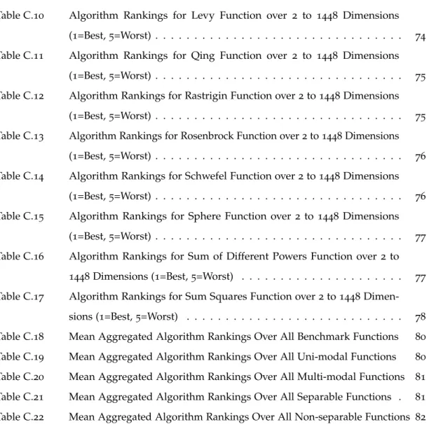
Figure3.1 Barchart Summarising Prevalence of Problems With Certain Features
Present in Each Benchmark Test Suite . . . 47
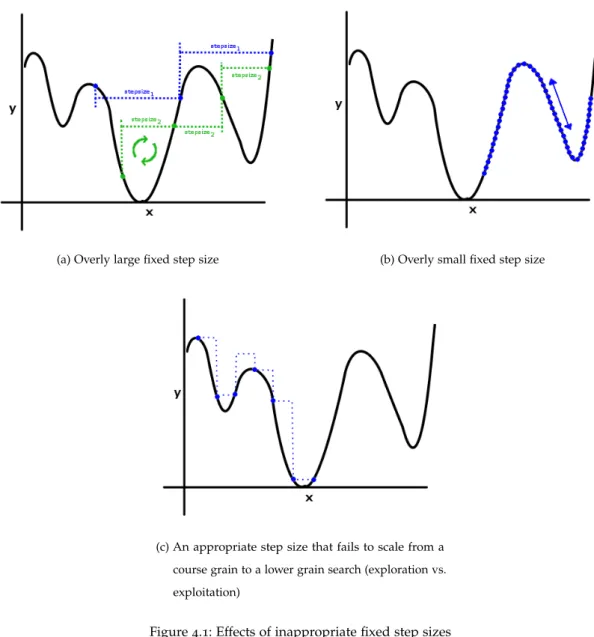
Figure4.1 Effects of inappropriate fixed step sizes . . . 53
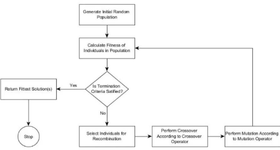
Figure4.2 Definition of a neighbourhood of a solution sol using the stepsize parameter and the stochastic generation of a neighbouring solutionsol2 64 Figure4.3 Basic operation of a typical genetic algorithm implementation . . . 68
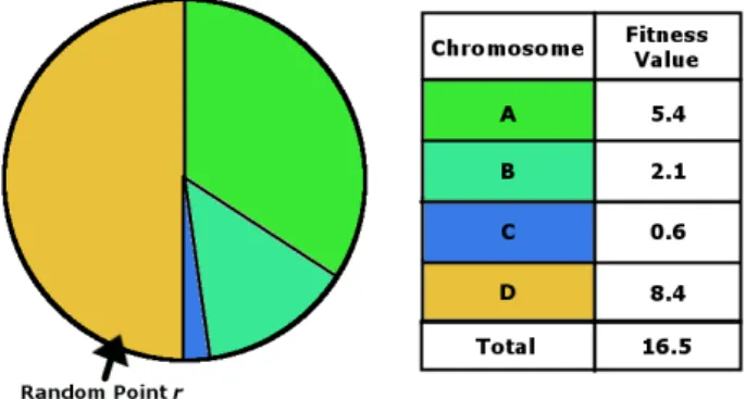
Figure4.4 Roulette Wheel Selection example showing a single selection over a population of four individuals. Each individual, A,B,C and D represent a32.7%,12.7%,3.6% and51% portion of the roulette wheel respectively. Random pointrselects the portion representing chromosome D similar to a hypothetical roulette ball . . . 70
Figure4.5 Tournament selection, where t =8(tournament size) . . . 72
Figure4.6 Uniform Crossover . . . 73
Figure4.7 One-point Crossover . . . 73
Figure4.8 Uniform Mutation: wherexis transformed tox0. . . 75
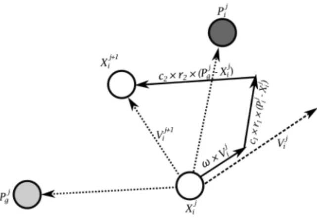
Figure4.9 Velocity and Position Update in PSO . . . 88
Figure4.10 Production of a mutant vector V~i from the scaled difference vector (X~r2−X~r3) . . . 109
Figure5.1 Taken from [58], This figure shows two steps of SMBO (EGO) for the optimization of a 1D function. The true function is shown as a solid line, and the circles denote our observations. The dotted line represents the mean prediction of a noise-free Gaussian process model (the DACE model), with the grey area representing its uncertainty. Expected im-provement, EI, (scaled by the authors for visualisation) is shown by a dashed line. . . 128
Figure6.1 Example of a parameter configuration file compiled from the individual problem-dimension configurations obtained from SMAC . . . 137
Figure6.2 Result Obtained from DE Implementation (tuning at 50,000 function evaluations) vs. Untuned Version . . . 140
Figure7.1 Examples of Successful Tunings of RMHC and SSGA Using SMAC on Ackleys Function and Alpine n.1 . . . 143
Figure7.2 Example of GA Continuing to Progress Beyond10,000Function
Evalu-ations for Ackley’s Function . . . 147
Figure7.3 SSGA Performance Results Comparison (Irace Tuned) Example -10,000 and50,000Tuning Evaluation Budgets . . . 148
Figure7.4 SSGA: Divergence of Performance between10,000and50,000Tuning Evaluation Budgets of SMAC and Irace . . . 149
Figure7.5 Example showing divergence between parameter tuning evaluation budgets for PSO (Alpine n.1 Function) at dimensions 11-16 and re-convergence occuring at dimension128 . . . 150
Figure7.6 Plots showing individual values for each tuned parameter from our original5parameter configurations sets obtained from SMAC . . . 151
Figure7.7 Comparison of Performance (Median Solution Quality of20Independent Repeats) Against the Chung-Reynolds Function Between Original and Extended Scale PSO Experiments . . . 153
Figure7.8 Mean Aggregate Ranking for Each Dimensionality and Pooled Mean Rank Over Every n Data Points Over All Benchmark Functions (where n=5) . . . 157
Figure7.9 Mean Aggregate Ranking for Each Dimensionality and Pooled Mean Rank Over Every n Data Points Over All Uni-modal Functions (where n=5) . . . 159
Figure7.10 Mean Aggregate Ranking for Each Dimensionality and Pooled Mean Rank Over Every n Data Points Over All Multi-modal Functions (where n=5) . . . 159
Figure7.11 Mean Aggregate Ranking for Each Dimensionality and Pooled Mean Rank Over Every n Data Points Over All Separable Functions (where n=5) . . . 162
Figure7.12 Mean Aggregate Ranking for Each Dimensionality and Pooled Mean Rank Over Every n Data Points Over All Non-separable Functions (wheren=5) . . . 162
Figure E.1 Ackley Function no.1in its2-dimensional form . . . 132
Figure E.2 Alpine Function no.1in its2-dimensional form . . . 133
Figure E.3 Bent Cigar Function in its2-dimensional form . . . 134
Figure E.4 Brown Function in its2-dimensional form: (a) and (b) shows the func-tion’s full domain, and (c) and (d) shows the function with domain limited to−16xi61 . . . 135
Figure E.6 Deflected Corrugated Spring Function in its2-dimensional form . . . . 137
Figure E.7 Exponential Function in its2-dimensional form . . . 138
Figure E.8 Griewank Function in its2-dimensional form . . . 139
Figure E.9 Inverted Cosine Wave Function in its2-dimensional form . . . 140
Figure E.10 Levy Function in its2-dimensional form . . . 141
Figure E.11 Qing Function in its2-dimensional form: (a) and (b) shows the function’s full domain, and (c) and (d) shows the function with domain limited to −26xi62 . . . 143
Figure E.12 Rastrigin Function in its2-dimensional form . . . 144
Figure E.13 Rosenbrock Function in its2-dimensional form: (a) and (b) shows the function’s full domain, and (c) and (d) shows the function with domain limited to−2.56xi 62.5 . . . 145
Figure E.14 Schwefel Function in its2-dimensional form . . . 146
Figure E.15 Sphere Function in its2-dimensional form . . . 147
Figure E.16 Sum of Different Powers Function in its2-dimensional form . . . 148
L I S T O F TA B L E S
Table3.1 Summary of the Proportion of Problems With Certain Features Present in Various Existing Test Suites Versus the Test Suite Constructed for this
Study . . . 47
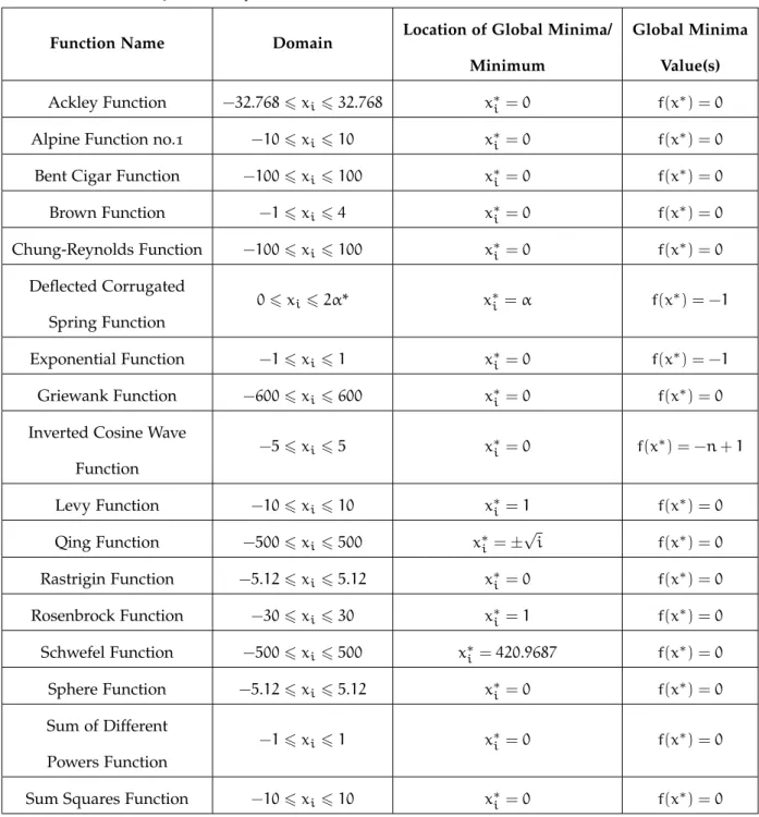
Table3.2 Summary of n-Dimensional Benchmark Function Suite . . . 49
Table7.1 Plot summary of problem dimensionalities where algorithm perform-ance between10k and50k evaluations diverge in favour of tuning at50k function evaluations . . . 146
Table7.2 Pooled Mean Rank Table Over All Functions . . . 157
Table7.3 Table of Pooled Mean Ranks Over All Uni-modal Functions . . . 160
Table7.4 Table of Pooled Mean Ranks Over All Multi-modal Functions . . . 160
Table7.5 Table of Pooled Mean Ranks Over All Separable Functions . . . 163
Table7.6 Table of Pooled Mean Ranks Over All Non-separable Functions . . . . 163
Table B.1 sep-CMA-ES Descriptive Statistics: Ackley to Deflected Corrugated Spring Functions (10,000Evaluation Tuning) . . . 33
Table B.2 sep-CMA-ES Descriptive Statistics: Ackley to Deflected Corrugated Spring Functions (50,000Evaluation Tuning) . . . 33
Table B.3 sep-CMA-ES Descriptive Statistics: Exponential to Rastrigin Functions (10,000Evaluation Tuning) . . . 34
Table B.4 sep-CMA-ES Descriptive Statistics: Exponential to Rastrigin Functions (50,000Evaluation Tuning) . . . 34
Table B.5 sep-CMA-ES Descriptive Statistics: Rosenbrock to Sum Squares Func-tions (10,000Evaluation Tuning) . . . 35
Table B.6 sep-CMA-ES Descriptive Statistics: Rosenbrock to Sum Squares Func-tions (50,000Evaluation Tuning) . . . 35
Table B.7 DE Descriptive Statistics: Ackley to Deflected Corrugated Spring Func-tions (10,000Evaluation Tuning) . . . 36
Table B.8 DE Descriptive Statistics: Ackley to Deflected Corrugated Spring Func-tions (50,000Evaluation Tuning) . . . 36
Table B.9 DE Descriptive Statistics: Exponential to Rastrigin Functions (10,000 Evaluation Tuning) . . . 37
Table B.10 DE Descriptive Statistics: Exponential to Rastrigin Functions (50,000 Evaluation Tuning) . . . 37 Table B.11 DE Descriptive Statistics: Rosenbrock to Sum Squares Functions (10,000
Evaluation Tuning) . . . 38 Table B.12 DE Descriptive Statistics: Rosenbrock to Sum Squares Functions (50,000
Evaluation Tuning) . . . 38 Table B.13 GA Descriptive Statistics: Ackley to Deflected Corrugated Spring
Func-tions (10,000Evaluation Tuning) . . . 39 Table B.14 GA Descriptive Statistics: Ackley to Deflected Corrugated Spring
Func-tions (50,000Evaluation Tuning) . . . 39 Table B.15 GA Descriptive Statistics: Exponential to Rastrigin Functions (10,000
Evaluation Tuning) . . . 40 Table B.16 GA Descriptive Statistics: Exponential to Rastrigin Functions (50,000
Evaluation Tuning) . . . 40 Table B.17 GA Descriptive Statistics: Rosenbrock to Sum Squares Functions (10,000
Evaluation Tuning) . . . 41 Table B.18 GA Descriptive Statistics: Rosenbrock to Sum Squares Functions (50,000
Evaluation Tuning) . . . 41 Table B.19 PSO Descriptive Statistics: Ackley to Deflected Corrugated Spring
Func-tions (10,000Evaluation Tuning) . . . 42 Table B.20 PSO Descriptive Statistics: Ackley to Deflected Corrugated Spring
Func-tions (50,000Evaluation Tuning) . . . 42 Table B.21 PSO Descriptive Statistics: Exponential to Rastrigin Functions (10,000
Evaluation Tuning) . . . 43 Table B.22 PSO Descriptive Statistics: Exponential to Rastrigin Functions (50,000
Evaluation Tuning) . . . 43 Table B.23 PSO Descriptive Statistics: Rosenbrock to Sum Squares Functions (10,000
Evaluation Tuning) . . . 44 Table B.24 PSO Descriptive Statistics: Rosenbrock to Sum Squares Functions (50,000
Evaluation Tuning) . . . 44 Table B.25 RMHC Descriptive Statistics: Ackley to Deflected Corrugated Spring
Functions (10,000Evaluation Tuning) . . . 45 Table B.26 RMHC Descriptive Statistics: Ackley to Deflected Corrugated Spring
Functions (50,000Evaluation Tuning) . . . 45 Table B.27 RMHC Descriptive Statistics: Exponential to Rastrigin Functions (10,000
Table B.28 RMHC Descriptive Statistics: Exponential to Rastrigin Functions (50,000 Evaluation Tuning) . . . 46 Table B.29 RMHC Descriptive Statistics: Rosenbrock to Sum Squares Function
(10,000Evaluation Tuning) . . . 47 Table B.30 RMHC Descriptive Statistics: Rosenbrock to Sum Squares Function
(50,000Evaluation Tuning) . . . 47 Table B.31 SA Descriptive Statistics: Ackley to Deflected Corrugated Spring
Func-tions (10,000Evaluation Tuning) . . . 48 Table B.32 SA Descriptive Statistics: Ackley to Deflected Corrugated Spring
Func-tions (50,000Evaluation Tuning) . . . 48 Table B.33 SA Descriptive Statistics: Exponential to Rastrigin Functions (10,000
Evaluation Tuning) . . . 49 Table B.34 SA Descriptive Statistics: Exponential to Rastrigin Functions (50,000
Evaluation Tuning) . . . 49 Table B.35 SA Descriptive Statistics: Rosenbrock to Sum Squares Functions (10,000
Evaluation Tuning) . . . 50 Table B.36 SA Descriptive Statistics: Rosenbrock to Sum Squares Functions (50,000
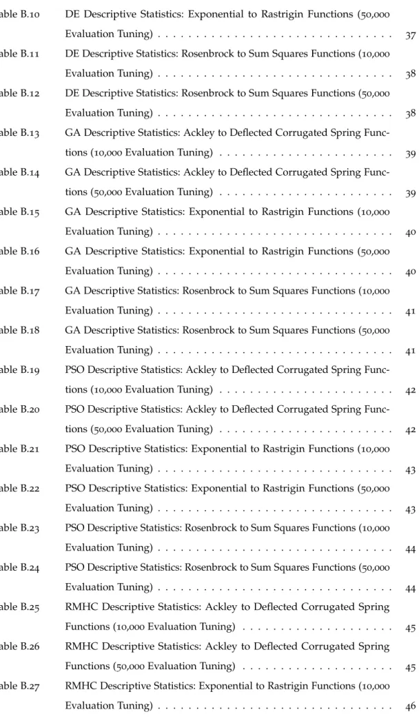
Evaluation Tuning) . . . 50 Table C.1 Algorithm Rankings for Ackley Function over 2to 1448 Dimensions
(1=Best,5=Worst) . . . 70 Table C.2 Algorithm Rankings for Alpine n.1Function over2to1448Dimensions
(1=Best,5=Worst) . . . 70 Table C.3 Algorithm Rankings for Bent Cigar Function over2to1448Dimensions
(1=Best,5=Worst) . . . 71 Table C.4 Algorithm Rankings for Brown Function over 2to 1448 Dimensions
(1=Best,5=Worst) . . . 71 Table C.5 Algorithm Rankings for Chung-Reynolds Function over2to1448
Di-mensions (1=Best,5=Worst) . . . 72 Table C.6 Algorithm Rankings for Deflected Corrugated Spring Function over2to
1448Dimensions (1=Best,5=Worst) . . . 72 Table C.7 Algorithm Rankings for Exponential Function over2to1448Dimensions
(1=Best,5=Worst) . . . 73 Table C.8 Algorithm Rankings for Griewank Function over2to1448Dimensions
(1=Best,5=Worst) . . . 73 Table C.9 Algorithm Rankings for Inverted Cosine Wave Function over2to1448
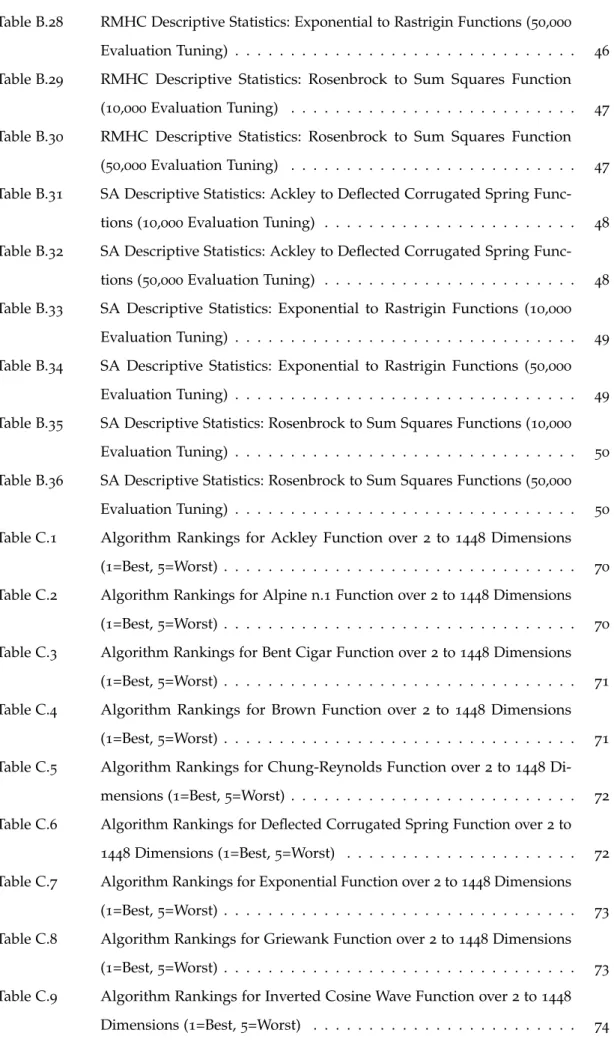
Table C.10 Algorithm Rankings for Levy Function over 2 to 1448 Dimensions (1=Best,5=Worst) . . . 74 Table C.11 Algorithm Rankings for Qing Function over 2 to 1448 Dimensions
(1=Best,5=Worst) . . . 75 Table C.12 Algorithm Rankings for Rastrigin Function over2to1448Dimensions
(1=Best,5=Worst) . . . 75 Table C.13 Algorithm Rankings for Rosenbrock Function over2to1448Dimensions
(1=Best,5=Worst) . . . 76 Table C.14 Algorithm Rankings for Schwefel Function over2to1448Dimensions
(1=Best,5=Worst) . . . 76 Table C.15 Algorithm Rankings for Sphere Function over 2 to 1448 Dimensions
(1=Best,5=Worst) . . . 77 Table C.16 Algorithm Rankings for Sum of Different Powers Function over 2to
1448Dimensions (1=Best,5=Worst) . . . 77 Table C.17 Algorithm Rankings for Sum Squares Function over2to1448
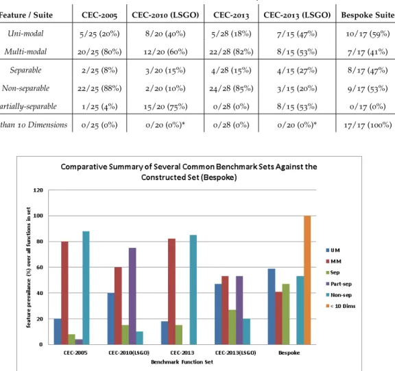
Dimen-sions (1=Best,5=Worst) . . . 78 Table C.18 Mean Aggregated Algorithm Rankings Over All Benchmark Functions 80 Table C.19 Mean Aggregated Algorithm Rankings Over All Uni-modal Functions 80 Table C.20 Mean Aggregated Algorithm Rankings Over All Multi-modal Functions 81 Table C.21 Mean Aggregated Algorithm Rankings Over All Separable Functions . 81 Table C.22 Mean Aggregated Algorithm Rankings Over All Non-separable Functions 82
L I S T O F A C R O N Y M S
acp Algorithm Configuration Problem
apt Automatic Parameter Tuning
asp Automatic Selection Problem
bcd Binary Coded Decimal
ccd Central Composite Design
cdiw Chaotic Descending Inertial Weight
cma-es Covariance Matrix Adaption - Evolution Strategy
criw Chaotic Random Inertial Weight
de Differential Evolution
ga Genetic Algorithm
gga Generational Genetic Algorithm
ils Iterated Local Search
nfl no free lunch (theorem)
pso Particle Swarm Optimisation
psosa Particle Swarm Optimisation Simulated Annealing
pso-tvac Particle Swarm Optimisation - Time Varying Acceleration Coefficients
rmhc Random Mutation Hill Climbing
rws Roulette Wheel Selection
sa Simulated Annealing
sga Simple Genetic Algorithm
shc Stochastic Hill Climbing
ssga Steady-State Genetic Algorithm
sus Stochastic Universal Sampling
Part I
1
I N T R O D U C T I O N T O T H E T H E S I S
1.1 i n t r o d u c t i o n
Human beings are a species of optimisers. Throughout history, advances in civilisation can be said to have been built, almost solely, on our ability to optimise the various processes essential to our survival. From our early ancestors gradually improving on their tools for hunting or gathering to developing more efficient means to automatically mass produce items of necessity during the industrial period, we owe much of our current, and relatively comfortable, state of being to our insatiable desire to ‘find something better’.
As our mathematics has developed, an ever increasing number of processes of increasing complexity are being modelled. Ever more complex models from the physical sciences, natural sciences and human sciences have provided us with new and interesting insights and new optimisation problems to solve. From molecular biology, for example, we have the problem of protein folding...
However, many of these real world problems can have very large search spaces; that is, the number of possible solutions to the problem can be incredibly large - increasing exponentially with the dimensionality of the problem. This makes it difficult for more traditional and exact optimisation methods, e.g., exhaustive search, to effectively search through all these possible solutions in a time that is acceptable. In terms of optimisation in continuous spaces; that is, where the problem variables are from the set of real numbers, these traditional approaches often make use of function derivatives. However, many continuous problems have search spaces that are inherently non-differentiable and thus inhibiting the use of these strategies.
For exactly these reasons, heuristic based optimisation methods - able to effectively search within arbitrarily large search spaces in a reasonable length of time - have become increasingly popular with several thousand associated publications even in the last year alone (2017). However, a fundamental theorem of any search based optimisation strategy - the No Free Lunch Theorem (NFL) - states that no single search algorithm, heuristic or otherwise, can be shown to exhibit higher than average performance when all possible problems are considered.
The consequences of the NFL therefore pose a problem to the users and developers of search based optimisation algorithms; specifically, what algorithm or algorithms will perform best on a given problem or set of problems of a certain type?
This problem, dubbed theAlgorithm Selection Problem(ASP) by Rice [112] in 1975, has been of some interest to researchers however despite its importance it has failed to gain widespread attention in the research community. Furthermore, of the works that do exist, none were found to address the issue of algorithm selection for large-scale optimisation problems - those of very high dimensionality. This is an important omission, and one we attempt to begin addressing - at least partially - because the exponential increase in search space volume that invariably results from increases to problem dimensionality means that the effectiveness - at least in terms of solution quality - of all search algorithms, including heuristic algorithms, diminishes with dimensionality. Some strategies may however remain reasonably effective on certain problems at higher dimensions - where their rate of decreasing performance with dimensionality is slower - but no data is yet available to even attempt to make such discriminations.
1.2 s t r u c t u r e o f t h e t h e s i s
We begin in Chapter2our review of the available subject matter. In this chapter we cover the subject of optimisation along with descriptions of some more ‘classical’ algorithmic approaches to addressing continuous optimisation problems.
In Chapter3, we provide a description of our selected suite of17benchmark functions used throughout the experiments in this thesis. Along with the descriptions, we also provide visual (2D) representations of each function we generated through sampling of the functions implemented. A review of the metaheuristic search-based optimisation algorithms being used in these studies is then provided in Chapter4.
We then briefly cover both the problem of algorithm selection and automatic parameter tuning (APT), in particular of the former - our selected tuning method, Sequential Model-based Algorithm Configuration (SMAC) in Chapter5.
Beginning our method part with Chapter6, attention is firstly given to the metaheuristic implementations developed for use in our experiments, including, for each approach, a list
and discussion of the various ‘tunable parameters’ configured by our selected APT described in Chapter5. To supplement this description, and to provide more specificity to our use of SMAC, Chapter7provides a brief description of the steps taken to tune each metaheuristic for each of our benchmark functions at each dimensionality.
Finally, in Chapter8, we blend our experimental methodology with individual findings and discussions and for each, provide our conclusions. These conclusions are then summarised at the end of the chapter along with a discussion of future work directions.
Part II
2
C H A P T E R 2: O P T I M I S AT I O N
2.1 i n t r o d u c t i o n
The task of optimisation has become one of the main staples of modern day science, finding utility in almost every scientific field of enquiry. In fact, Schwefel in [118] states:
“There is scarcely a modern journal, whether of engineering, economics or the social sciences, in which the concept ‘optimization’ is missing from the subject index.”
Given our long relationship with optimisation and its many successes, having been paramount to our continued advancement as a species for thousands of years, this is not too surprising.
However, as problems have become increasingly more complex, compounded with the fact that in many cases we do not know the mathematical formulation of our problem, we are less able to rely on some of our more ‘classical’ or exact methods to optimisation. This has led to the popularisation of stochastic optimisation methods, specifically those techniques such as metaheuristics and hyper-heuristics, that are more able to deal with these intractable problems in a reasonable time scale albeit with no guarantee of exact optimality. Therefore, metaheuristics and other stochastic approaches have their place in situations where a ‘good enough’ solution is acceptable or no known exact algorithm can find the optimal solutions in reasonable runtimes.
This chapter begins by discussing some of the background and terminology of optimisa-tion in general, including: a definioptimisa-tion of optimisaoptimisa-tion, an overview of how problem difficulty is defined and what this means to optimisation on the whole and a comparison of the main categories of optimisation: discrete vs. continuous and local vs. global optimisation. Next we present an overview of some of the more classical and exact methods to optimisation and how these approaches are less able to perform efficiently when problems being approached become larger and more complex. This leads us give a relatively concise discussion on the topic of metaheuristics, specifically how they are applied to help solve continuous optimisation problems.
2.2 g e n e r a l o p t i m i s at i o n
2.2.1 Terminology
Here we present some terminology useful to further discussions in this chapter.
2.2.1.1 Objective Function
An objective function is an encoding of the goal of some problem as a mathematical function or computational model used to measure the quality of a given solution in respect to the problem. It essentially represents the interface between an algorithm and the real problem and plays a crucial role in the guidance of a search algorithm though a given search space -without it the algorithm would have no clue as to how the solutions produced are performing. The problem goal, or goals in the case of multi-objective problems, can be defined as either being a minimisation goal, where the objective is to produce solutions with low values with respect to the objective function, or a maximisation problem where higher valued solutions are sought. When indirect solution representations are used within the algorithm - those that do not yet represent a solution in their current form i.e., they are encoded so must first be converted (decoded) into a form that can be directly evaluated by the objective function [17].
2.2.1.2 Feasible vs. Infeasible Solutions
Feasible solutions are all solutions within the search space of the problem which satisfy the constraints on the problems parameters - specifically, the hard constraints (see below) [17]. Conversely, infeasible solutions all violate at least one of the problems hard constraints.
2.2.1.3 Hard vs. Soft Constraints
Hard constraints placed on a problem are conditions which have to be satisfied in order for a solution to be feasible [17]. On the other hand, soft constraints are those which we would like to have satisfied but which are not essential; so a solution violating one or more soft-constraints would still be considered feasible [17]. A common way of handling soft constraints when searching for a solution to an optimisation problem is to have solutions incur a penalty if a soft constraint is not satisfied; possibly weighted by desirability. Therefore, the objective function of many problems are represented by the summation of penalties for the soft constraints [17]. This means that solutions that do not violate the soft constraints will be considered as being of a higher quality [17].
2.2.1.4 Local vs. Global Optimisation
The difference between local and global optimisation lies in the scope of the optimisation task. Local optimisation looks to optimise within a local feasible region [97], that is, to discover a local minimiser (or optimum) - the smallest objective value within some feasible neighbour-hood in the problem domain. A neighourneighbour-hood functionNdefines the neighbourhood of a solutions∈Sas a mappingN:S→2S which assigns to eachsa set of solutionsN(s)⊂S [135]. A solutions0∈N(s)is refered to as a neighbour ofs[135]. Therefore, given a domainS and a feasible neighbourhood of the domainN(s)⊂S, local optimisation seeks to find a local optimumx∗∈Nsuch thatf(x∗)6f(x)∀x∈N[135]. Global optimisation on the other hand is concerned with discovering the smallest objective value or values over the entire feasible domain of a function - a global optimum, also often referred to as the ‘best solution’. As before, given a domainS, global optimisation seeks to find a global optimums∗∈Ssuch that f(s∗)6f(s)∀s∈S[135]. The main outcome of optimisation is therefore to discover a global optimums∗of which many such solutions may exist [135]. Where many global optima may be present (it is not always known), the outcome may be defined as attempting to discover all of the global optima in order to generate alternative choices of solution [135].
2.2.1.5 Best Solution
Using a term like the best solution implies that there must be more than one solution, all of which are considered to have differing levels of value [50]. The meaning of best, in terms of quality, is quite often depends on the actual problem, the solution method and any allowed tolerances [50]. Some types of problem have exact answers where the term ‘best’ has an absolute definition [50] - in optimisation terms, ‘best’ in these instances refers to a problems single global optimum. Other problems however can have several global optima, so ‘best’ in these situations is more of a relative term [50]
2.2.1.6 Discrete vs. Continuous Optimisation
Discrete optimisation involves the optimisation of problems which are characterised by a finite number of states accepted by their input parameters; on the other hand, continuous problems are typically those that take their solutions from an uncountably infinite set of solutions whose parameters are members of the set of real values - of which there are no discontinuities [97]. However, given that digital computer technologies cannot provide the kind of precision required of a ‘true’ continuous solution, the set of possible solutions will be far less than uncountably infinite albeit still intractably large.
Although the practical optimisation of both types of problem can be approached using similar methods - at least in terms of inexact heuristic methods - there are nuances found for each type of problem that need to be taken into account in order to optimise effectively. For example, continuous optimisation problems are considered easier to solve than discrete problems as their typical smoothness make it possible to work out the functions behaviour at all points close to a pointxby using objective and constraint information [97]. On the other hand, the behaviour of the objective function may change drastically between points - which are deemed close by some measure of distance [97].
2.2.2 A Formal Definition of an Optimisation Problem
Burke and Kendall in [17] define optimisation as trying to find the best solution possible from amongst all possible solutions. They state further that optimisation can therefore be considered as the task of modelling the problem to be solved as a mathematical evaluation (or objective) function representing the quality of a solution and then search through the space of all possible solutions in order to find one that either minimises or maximises this function [17].
The canonical form for an optimisation problems is usually stated as the minimisation of the objective function subject to constraints placed on its variables and expressed as [97,6]:
minf(x) :x∈Rn subject to gj(x)>0, j={1,2,. . .,J} hk(x) =0, k={1,2,. . .,K} such that: x(L)i 6xi6x (U) i , i={1,2,. . .,n} (2.1)
wheref(x)is the function being optimised,gj(x)areJinequality constraints and hk(x) represent theKequality constraints [6].
2.2.3 Problem Difficulty
Michalewicz and Fogel in [90] state several different reasons why real-world optimisations are difficult to solve effectively:
• The problem is so complex that in order to determine any answer whatsoever requires the use of such simplified models of the problem domain that any solution found is essentially useless
• The objective function is noisy or varies over time therefore requiring that an entire series of solutions are required as opposed to a single solution
• The search space is so heavily constrained that even finding one feasible solution to the problem is difficult
2.2.3.1 Complexity and P vs. NP
Complexity refers to the study of how difficult an optimisation problem is to solve [17]. Here, problems are classified according to the properties of optimisation algorithms where roughly speaking, a problem is classified as being ‘hard’ if there exists no known fast solver and ‘easy’ otherwise [29].
The first key concept in computational complexity is that of problem size which is rooted in the dimensionality of a given problem - that is, the number of problem parameters - and the size of the set of values of which each of the problem parameters can be set [29].
The second key concept relates to algorithms rather than to the problems themselves, that of the running-time [29]. Running-time is the number of “elementary” operations required of an algorithm before it terminates when running against a given problem - in general, the intuition of computational complexity is that larger problems will require more computational time to solve, although this is not always true [29]. The best known definitions of the ‘hardness’ of a problem is a relationship between the size of the problem being solved to the worst-case runtime of the algorithm to be used to solve it. This is encapsulated as a formula that defines an upper bound on runtime of the algorithm as a function of the problem size [29]. Basically, shorter running times are expected when this formula is a polynomial or longer when the formula is ‘super-polynomial’ such as exponential [29].
The final key concept of computational complexity relates to the concept that it is possible to transform one problem into another through an appropriate mapping which may or may not be reversible. This is referred to asproblem reduction[29].
1. A problem can be said to belong to the class P (polynomial) if there exists at least one algorithm capable of solving it in polynomial time [29]
2. A problem can be said to belong to class NP (Non-deterministic polynomial) when it can be solved by some algorithm, specifically a non-deterministic turing machine, with no runtime guarantees, and its solution can be tested in polynomial time [29]. P can be considered as a subset on NP since a solver with a polynomial runtime can also be used to test solutions in polynomial time [29]
3. A problem is said to belong to the class NP-complete when it belongs to the class NP and another problem in NP can be reduced to this particular problem by an algorithm that runs in polynomial time [29]
4. A problem belongs to the class NP-hard if (i) it is at least as difficult as any problem in NPcomplete, but (ii) where solutions cannot be necessarily tested in polynomial time -the canonical example being -the halting problem [29]
One of the ‘grand’ challenges in complexity theory is to provide a proof thatP=NPor conversely thatP6=NP, in other words, is the class P and the class NP in fact the same class - or not, in the latter case [29]. It should be noted that the proof required of the latter case will need to be acquired through the application of complex mathematics, but for the former, ‘simply’ showing that an algorithm exists that can solve at least problem of class NP-complete would provide enough of a proof [29].
2.3 c l a s s i c a l o p t i m i s at i o n m e t h o d s
Before continuing on further to discuss stochastic optimisation, it is worth outlining some of the existing ‘classical’ mathematical optimisation techniques. Wehrens and Buydens [142] categorise the following methods under two headings:strongmethods andweakmethods.
Strong methods make certain assumptions about the structure of the solutions space; if the assumptions made are correct then strong methods are both fast and reliable - however, it they are incorrect the methods will never manage to find the global optimum even through increased repetitions [142]. They are often used in the final part of the optimisation of difficult problems where the region of the global optimum has been found but an exact solution has yet to be discovered [142]. Additionally, they find utility where problem dimensionality is low [142].
Weak problems, on the other hand, make very little - if any - assumptions about the search space but at a cost to their effectiveness and/or performance and should only be used when there is no other option [142]. Each essentially samples the search space in the hope of discovering good solutions quickly [142] The quintessential example of an weak method is that of exhaustive enumeration of the search space, a technique whose use is infeasible for all but the smallest of problem instances [142]. They tend to make use of a random component in generating solution instances, given the fact they also use no assumptions - repeatability then tends to be low as repeated runs of these approaches typically produce very different results [142].
Between these two classes lies anintermediate class encapsulating approaches such as metaheuristics and other stochastic algorithms. Metaheuristics will be discussed later in this chapter in section2.4.5.3and specific methods described in Chapter4.
2.3.1 Strong Methods
2.3.1.1 Gradient-based Optimisation Methods
g r a d i e n t a s c e n t The first gradient-based method that will be discussed is that of Gradient Ascent - or Descent if dealing with minimisation. Here, the basic idea is to find the slope of the function to be optimised, from the current point, and move up the hill towards the maxima at its peak [82]. Progress continues until the slope of the function reaches zero - which may or may not have occurred around a function maxima. Since progress cannot continue where the slope equals zero, it is possible for gradient ascent to converge elsewhere, such as: (i) at minima of the function and (ii) atsaddle points. The gradient ascent method does not require the computation or knowledge off(x), but it does however make the assumption that the first derivativef0(x)can be known and calculated [82]. The procedure for this method is quite straightforward for both the1-dimensional and the n-dimensions cases.
In1-dimension, a random initial point is selected. We then continually add to it a portion of its slope i.e.,x←x+αf0(x)- whereαis a small positive value [82]. This process continues until the slope reaches zero and therefore x is unable to change further [82]. For the n-dimensional case, the slope at the current point is simply replaced with the gradient so that ¯x←x¯+α∇f(x)¯ . There are a couple of known problems with gradient descent, one has already been discussed - that of search progress being unable to continue when a slope not found at an optima equals zero. The other issue is speed of convergence. The reason behind this second issue is that as the slope approaches zero at the maximum, the value for x will overshoot the peak - landing
on the other side of the hill - and may do this many times before reaching the maximum. The cause of this is due to the step sizeαbeing based solely on the slope of the function at the current position. If a slope is very steep,αwill be large even if it is not required. One way to deal with this is to tune the value ofαto the particular problem instance being tackled. Another way, if the second derivative of the function,f00(x), can also be calculated, would be to abandon the gradient ascent method altogether, opting instead for Newtons Method, a variation of gradient ascent described next.
n e w t o n’s m e t h o d This variation on gradient ascent/descent involves the use of the second derivative, i.e.x←x−αff000(x)(x) of the function such thatαis dampened as the algorithm approaches a slope of zero [82]. This means that the algorithm will now converge to any kind of zero slope - maxima, mimima, saddle points and to points of inflection [82]. Additionally, the multidimensional case of the second derivative is not as straightforward to compute as the gradient∇f(x)¯ was for the first derivative, but is instead a multi-dimensional Hessian matrixHf(x)¯ comprised of partial second derivatives over each dimension [82]. This extra complexity is compounded by the fact that newtons method divides by the second derivative, requiring that inverse hessian matrix be calculated [82].
Since the second derivative is being used, the algorithm maintains all the information required to identify whether it has reached a maximum solution (or minimum point in the case of minimisation) as opposed to other points of zero slope discussed previously. This is due to the fact that the second derivative will have negative value when a maximum point is met and positive otherwise [82].
The use of the functions second derivative still does not solve the overall problem of local search methods however, in that it can still converge to local optima rather than the global optima [82]. One simple method of constructing a global search algorithm from both gradient ascent and newtons method is to place these algorithms in a loop such that as a local optima is discovered, the algorithm may be restarted from a random position in the search space - keeping track of the best optimum found so far - in the hope of finding better optima which hopefully lead to the global optima [82]. This is essentially the same approach taken for derivative-free hill climbing algorithms when looking to search for global optima - see Chapter4Section4.2.2.1for more details on using restarts for global optimisation.
2.3.1.2 Response Surface Methods
Originating from the area of experimental design, response surface methods make the as-sumption that the response surface (objective function landscape / fitness landscape) can be parameterised under a simple functions containing a single optimum [142]; that is, these
methods aim to estimate the response surface by choosing parameters in an intelligent way [142]. A common implementation is known as a central composite design (CCD) which makes use of2N points (factorial points) [70] combined with2Npoints (axial points) [70] and one central points [142,70].
2.3.1.3 Simplex Methods
The Nelder-Mead Simplex algorithm, or simplex algorithm, was introduced in1965by Nelder and Mead in [94] for multidimensional unconstrained optimisation problems. The approach achieves this without derivative information - using only the returned objective function values at given points - and do not attempt to approximate a gradient at any point [122]. From its name, the Nelder-Mead Simplex algorithm is simplex based1
Simplex-based algorithms begin with an initial working simplex composed ofn+1solution points considered as the vertices of the simplex and a corresponding set of objective function valuesfj:=f(xj) :j={1,2,. . .,n} [122]. It is a requirement of the method that the initial vertices do not lie in the same hyperplane, that is, the simplex should be non-degenerate [122].
To execute the algorithm, a sequence of transformation operators are applied to the simplex which are determined by testing one or more test points and comparing these with the objective values of the vertices [122]. The general procedure can be stated simply as [122]
1. Generate an initial working simplex
2. While termination criteria not satisfied:
a) calculate the information relevant to testing termination criteria
b) transform the current working simplex
3. Return the objective value of the best vertex of the final simplex
There are four fundamental transformation operators, each controlled by a parameter: reflectionα, contractionβ, expansionγand shrinkδ[122]. Each of the four parametersα,β, γandδmust satisfy the following constraints [122]:
• 0 < α < γ > 1,0 < β < 1,0 < δ < 1
The most common values of these parameters that satisfy the constraints are:α=1,β=0.5, γ=2andδ=0.5[122].
t r a n s f o r m at i o n s t e p s Transformation of the current simplex follows three steps [123,122]:
1. determine the worst, second-worst and best vertices in the simplex:h,sandlrespectively as in:
fh=max
j fj, fs=maxj6=hfj fl =minj6=hfj
2. A new centroid is computed for the best side - opposite from the worst vertex - by: c= n1Pnj=0
j6=h
xj
3. Calculate the new working simplex by:
a) First attempt to replace the worst vertex with a new vertex through reflection...
• If the new vertexxris better than the second best vertexxsbut is not better than the best vertexxl then simply accept the new vertex, replacingxhand continue on to the next iteration
• If the new reflected vertexxris actually better than the best vertexxl, attempt to explore further by expandingxr toxeby:
xc=c+γ(xr−c)
• The vertexxhis the replaced by the better of the verticesxr andxe
b) If the reflected pointxr was found to be worse than the second best vertexxs then this suggests that the region ofxr is not a promising direction so we perform contraction on the simplex by: xc=c+β(xh−c)
• if the new contracted vertexxcis better thanxhthenxhis replaced byxcand move to the next iteration, that is:xh←xc
• If the contracted vertexxcis worse thanxhwe must resort to the final trans-formation, the shrink operator which transforms the entire simplex by main-taining the current best pointxl and modifying all others relative to it. Thejth new point is calculated using:
xj=xl+δ(xj−xl)
Termination is then determined by the following criteria:
1. Iteration budget has been exhausted
2. The minimum size for the simplex ha been reached
The main advantage of simplex methods according to [122] is that it succeeded in achieving a good minimisation of the objective function over a number of numerical trials and does so over a relatively low number of objective function evaluations. However, a disadvantage given is that “numerical breakdown” of the algorithm occurs in practice resulting in requiring an “enormous” number of iteration and making very little progress toward the minimum - even when the simplex is nowhere near the minimum [122].
2.3.2 Weak Methods
2.3.2.1 Random Search
This very simple approach involves sampling the search space at random, maintaining the best found and terminating when the time budget is exceeded [142]. As such, this is not an approach that is widely used [142] given the multitude of other more successful methods available - of which some are close in terms of their simplicity (See Hill Climbing Approaches, Chapter4- Section4.2). In fact, the only class of problem that this approach is expected to perform as well as any other is that of needle-in-the-haystack problems - where the entire search space is completely ‘flat’ except for a single point, and so no information involving the proximity of the optimum from the current location can be obtained by any existing algorithm [142].
2.3.2.2 Sampling Methods
A somewhat more feasible weak method is to sample the search space using a grid of a pre-determined size [142] - aptly referred to asgrid searchmethods. When promising regions are identified, grids with smaller spacings may be placed in these locations in order to perform a more fine grained search [142]. These approaches suffer more than most from the curse of dimensionality (Chapter3- Section3.2) where as the number of problem dimensions increases the number of samples required to form the grids increases exponentially [142]. Another disadvantage is that since points between the samples are not known so good solutions and regions smaller than the spacing of the grid may be missed [142].
2.4 m e ta h e u r i s t i c o p t i m i s at i o n
2.4.1 What is a Metaheuristic?
The name metaheuristic is derived from a combination of the Greek prefix ‘meta’, meaning beyond - in terms of high-level and ‘heuristic’ from the greek word ‘heuriskein’ meaning ‘to search’ [39]. This combination can therefore translated roughly to ‘high-level search’. Although this etymology may provide us with a loose idea of what it may mean to be a metaheuristic, unfortunately, no one definition of metaheuristic available in the literature seems to capture everything that it means to be a metaheuristic and so several will be presented in this section for comparison.
As stated by Burke and Kendall in [17], Glover first used the term metaheuristics in1986 in [39] and defines it as2:
“A meta-heuristic refers to a master strategy that guides and modifies other heuristics to produce solutions beyond those that are normally generated in a quest for local optimality. The heuristics guided by such a meta-strategy may be high level procedures or may embody nothing more than a description of available moves for transforming one solution into another, together with an associated evaluation rule”
Stutzle in [131], found in [11], offers another quite explanatory definition:
“Metaheuristics are typically high-level strategies which guide an underlying, more problem specific heuristics, to increase their performance. The main goal is to avoid the disadvantages of iterative improvement and, in particular, multiple descent by allowing the local search to escape from local optima. This is achieved by either allowing worsening moves or generating new starting solutions for the local search in a more “intelligent” way than just providing random initial solutions. Many of the methods can be interpreted as introducing a bias such that high quality solutions are produced quickly. This bias can be of various forms and can be cast as descent bias (based on the objective function), memory bias (based on previously made decisions) or experience bias (based on prior performance). Many of the metaheuristic approaches rely on probabilistic decisions made during the
search. But, the main difference to pure random search is that in these algorithms randomness is not used blindly but in an intelligent, biased form.”
A less formal definition of metaheuristics, as defined by Sean Luke in [82], is that metaheuristics comprise a general class of optimisation algorithms - forming the main sub-field of stochastic optimisation - that make use of some level of randomness in order to find the solution to ’hard’ problems [82].
Blum and Roli in [11] provide a summary of the fundamental properties in which they feel characterise metaheuristics:
• “Metaheuristics are strategies that “guide” the search process”
• “The goal is to efficiently explore the search space in order to find (near-)optimum solutions”
• “Techniques which constitute metaheuristic algorithms range from simple local search procedures to complex learning processes”
• “Metaheuristic algorithms are approximate and usually non-deterministic”
• “The may incorporate mechanisms to avoid getting trapped in confined areas of the search space”
• “The basic concepts of metaheuristics permit an abstract level description”
• “Metaheuristics are not problem specific”
• “Metaheuristics may make use of domain-specific knowledge in the form of heuristics that are controlled by the upper level strategy”
• “Todays more advanced metaheuristics use search experience (embodied in some form of memory) to guide the search”
They continue to then offer their own short definition of a metaheuristic, as [11]:
“In short we could say that metaheuristics are high level strategies for exploring search spaces by using different methods. Of great importance hereby is that a dynamic balance is given between diversification and intensification . . . ”
For our purposes, we define a metaheuristic to be an algorithm making use of some for of randomness, comprised of one or more high-level heuristics whose task it is to drive and control a set of lower-level search heuristics in their quest to discover ‘good enough’ solutions to ‘hard’ optimisation problems.
2.4.2 Exploration vs. Exploitation in Metaheuristics
A common theme in all metaheuristics is that of the trade-off between exploration and exploit-ation [6] - also referred to a diversification and intensification respectively [11]. Exploration refers to the force in a metaheuristic, provided by its operators, that diversifies solutions main-tained by the algorithm from the search space [6]. This divergent behaviour of the algorithm encourages a global search behaviour [6]. Exploitation on the other hand refers to how well the metaheuristic operators are able to use information from previously discovered solutions in order to focus the search on specific regions of the search space [6]. Metaheuristics exist on a spectrum depending on how much of each property is displayed i.e., some metaheuristic approaches can be more exploitative than explorative and vice-versa [6].
On the extreme ends of the scale, an example of a purely explorative search can be observed in the trivial random search algorithm which involves randomly selecting solutions in the search space for a given number of iterations [6]. Examples of purely exploitative search are hill climbing algorithms (Chapter4- Section4.2) that perform small incremental steps in the space while new improvements are discovered or no further steps can be taken without finding a worsening solution [6]. Most metaheuristics, however, offer the ability to tune these aspects through the parameters used by their operators [6].
The exploitative and explorative nature of metaheuristics, along with their effective use of randomness, give them several advantages over classical (exact) optimisation methods. Bandaru and Deb illustrate this in [6] with the following list:
• Metaheuristics are able to find ‘good enough’ solutions to computationally ‘easy’ prob-lems with a large input complexity [6]
• They can find ‘good enough’ solutions for NP-hard problems (see Section2.2.3.1) [6]
• As opposed to most classical optimisation approaches, metaheuristics make use - and indeed, do not require - gradient information about the objective function and can therefore be applied to non-analytic, black-box or simulation-based objective functions [6]
• Most metaheuristic algorithms are capable of escaping from local optima [6]
• Due to the above ability to escape local optima, metaheuristics can better deal with uncertainties related to the objectives [6]
• Multiple objectives can be handled by most metaheuristics given minor algorithmic modifications [6]
2.4.3 Problems Addressed by Metaheuristics
The types of problem addressed by metaheuristics are those where
• The size of the solution space is large enough to make the use of exhaustive or exact algorithms infeasible,
• There is no known deterministic algorithm to solve the problem at all or within a reasonable time frame, and
• Problems where there is little knowledge of the domain that can be used to construct an optimal solution[82].
• A near-optimal solution to a problem is acceptable as opposed to the searching for the exact optimal solution [6]. Metaheuristics do not come with any guarantees of optimality.
2.4.4 Categorisations of Metaheuristics
Several different categorisations of metaheuristics, based on a variety of properties, have been made over the years. Unfortuanately, there is little consensus as to a single scheme for categorising metaheuristics from the list given in the next subsections, they are often used interchangeably in the literature and even combined for increased specificity.
2.4.4.1 Nature-inspired vs. Non-nature Inspired Metaheuristics
One method used to classify metaheuristics is by basing this classification on the conceptual origins of the approach [11]. In metaheuristic research, these origins roughly fall into the category of either being inspired by natural processes (Genetic Algorithms (GA) and Particle Swarm Optimisation (PSO)) or “artificial” (Tabu Search and ILS) in the sense that nature was not queried for insight. Blum and Roli [11] do not consider this classification very meaningful for two reasons. The first is that many ‘hybrid’ approaches do not fit cleanly into either class - and in fact, may fit both simultaneously [11]. The second reason given is that it is often difficult to attribute even some non-hybrid metaheuristics to either class, for example, the use of memory in Tabu search could also be considered as being nature inspired [11].
2.4.4.2 Single-solution vs. Population-based Metaheuristics
Another characteristic that may be used for classifying metheuristics is whether one or more solutions are being utilised at once [11]. Metaheuristic algorithms that operate only on a single solution are often referred to astrajectory methodswhich include the set of local search algorithms such as: Iterated Local Search (ILS), Simulated Annealing (SA) and Tabu Search [11]. What all these algorithms have in common is their property of describing the path , or trajectory, through the search space [11]. In contrast, population based metaheuristics such as: Particle Swarm Optimisation (PSO), Genetic Algorithms (GA) and Differential Evolution (DE), focus on the descriptions of the evolution of multiple, often related, solutions in the search space [11]. Another way of referring to these classifications is asLocal vs. Global Optimisation Metaheuristics- typically single solution metaheuristics are only employed for local search whereas population-based approaches are able to search for a globally optimum solution to a given problem.
2.4.4.3 Dynamic vs. Static Objective Function
Metaheuristics can also be classified by the way in which they might make use of the objective function [11]. Some approaches use the objective function in the same way it is provided - as a ‘black-box’ - where others such as guided local search make modifications to the objective function as the search progresses [11]. The logic behing this approach is to enable the algorithm to escape from local optima by changing the search landscape itself [11].
2.4.4.4 One vs. Many Neighbourhood Structures
The majority of metaheuristics make use of only a single neighbourhood structure throughout the search process. What this means is that the topology of the search landscape does not change [11]. Others, the canonical example being Variable Neighbourhood Search (VNS), make use of a set of neighbourhood topologies allowing for the algorithm to switch between then in order to diversify the search [11].
2.4.4.5 Memory vs. Memoryless Metaheuristics
Another classification scheme is to focus on whether or not the metaheuristic makes use of search history / trajectory information - these days considered to be a fundamental component of sucessful metaheuristics [11]. Memoryless algorithms, such as Simulated Annealing (SA), carry out a Markov process - where the information used to decide where the search should explore next is taken exclusively from the current solution [11]. For Memory algorithms, a further delineation can be found in the various ways that an algorithm may make use of
memory - usually considered between the categories of short or long-term memory [11]. Short-term memory approaches typically maintain only information about the previous few iterations, the last few solutions found and decisions made [11]. Long-term memory approaches on the other hand make use of a large set of various ‘synthetic’ parameters about the search [11].
2.4.5 General Concepts
2.4.5.1 Solution Representations Used in Metaheuristics
In order to develop solutions to a given problem; that is, to provide input to the objective function representing the problem, a suitable solution representation for use in optimising the problem in the context of metaheuristics must be selected. There are several drawbacks and advantages to the use of each type of solution representation discussed here, however the selection of a representation is often heavily influenced by the problem being solved. Any change to solution representation will often require a subsequent change to the objective function and in effect, the nature of the search space will also change. For example, it may be tempting to use a representation simply because it feels more natural and intuitive but some search spaces based on a representation (and it’s corresponding objective function) may well be more rugged, sparse, deceptive or of a larger scale than other spaces defined by other representations and functions. The solution representation also determines how the search operators might create neighbourhoods and how the objective function will be evaluated; for example, a representation requiring heavy or complex conversion by the objective function will require more time and computational resources. Objective functions are considered to be one of the main bottlenecks in search, so it is always prudent to minimise computation costs here where possible. All in all, it is important to keep the nature of the resulting search space in mind when selecting a representation as the efficiency of search is very much determined by it. In the following paragraphs, since we work primarily with a vector-based representation3
, we outline several of the more common vector-based representations and how they are typically used.
(a) b i na r y r e p r e s e n tat i o n The simplest of the common representations used, the binary representation, is one in which each solution is held as a vector of bits where each bit or sub-sequence of bits represents some parameter of the problem being solved [29]. For a given problem, a practitioner should: (i) ensure that it is clear how the binary string is to be