Durham Research Online
Deposited in DRO:22 February 2018
Version of attached le:
Accepted Version
Peer-review status of attached le:
Peer-reviewed
Citation for published item:
Eryilmaz, S. and Coolen, F.P.A. and Coolen-Maturi, T. (2018) 'Mean residual life of coherent systems consisting of multiple types of dependent components.', Naval research logistics., 65 (1). pp. 86-97.
Further information on publisher's website: https://doi.org/10.1002/nav.21782
Publisher's copyright statement:
This is the accepted version of the following article: Eryilmaz, S., Coolen, F.P.A. Coolen-Maturi, T. (2018). Mean residual life of coherent systems consisting of multiple types of dependent components. Naval Research Logistics 65(1): 86-97, which has been published in nal form at https://doi.org/10.1002/nav.21782. This article may be used for non-commercial purposes in accordance With Wiley Terms and Conditions for self-archiving.
Additional information:
Use policy
The full-text may be used and/or reproduced, and given to third parties in any format or medium, without prior permission or charge, for personal research or study, educational, or not-for-prot purposes provided that:
• a full bibliographic reference is made to the original source
• alinkis made to the metadata record in DRO
• the full-text is not changed in any way
The full-text must not be sold in any format or medium without the formal permission of the copyright holders. Please consult thefull DRO policyfor further details.
Mean residual life of coherent systems consisting
of multiple types of dependent components
Serkan Eryilmaz, Frank P.A. Coolen
yand Tahani Coolen-Maturi
zFebruary 20, 2018
Abstract
Mean residual life is a useful dynamic characteristic to study reliability of a system. It has been widely considered in the literature not only for single unit systems but also for coherent systems. This paper is concerned with the study of mean residual life for a coherent system that consists of multiple types of dependent components. In particular, the survival signature based generalized mixture representation is obtained for the survival function of a coherent system and it is used to evaluate the mean residual life function. Furthermore, two mean residual life functions under di¤erent conditional events on components’ lifetimes are also de…ned and studied.
Key words. Dependence; Mean residual life; Minimal survival signature; Reliability; Survival signature
1
Introduction
The study of mean residual life of a coherent system has attracted a great deal of attention in reliability theory. Consider a system with components which has two possible states; (x1; :::; xn) = 1if the system is functioning and (x1; :::; xn) = 0if the
system has failed, wherexi = 1 if the ith component is functioning andxi = 0 if the
ith component has failed. The function (x1; :::; xn) is called the structure function.
A system with structure function (x1; :::; xn) is coherent if it is nondecreasing in
each argument, and each component i is relevant to the performance of the system, i.e. (x1; :::; xi 1;0; xi+1; :::; xn) = 0 and (x1; :::; xi 1;1; xi+1; :::; xn) = 1 for some
states x1; :::; xi 1; xi+1; :::; xn of other components 1;2; :::; i 1; i+ 1; :::; n. Besides
the classical de…nition of the mean residual life, di¤erent mean residual life functions Department of Industrial Engineering, Atilim University, 06836, Incek, Ankara, Turkey, e-mail: [email protected]
yDepartment of Mathematical Sciences, Durham University, Durham, United Kingdom zDurham University Business School, Durham University, Durham, United Kingdom
have been de…ned and studied in the literature for a coherent system. For a coherent system with lifetime T and components’lifetimes T1; :::; Tn; the usual mean residual
life is de…ned by E(T t j T > t): Navarro and Hernandez (2008) studied the mean residual life function of a system whose reliability function can be written as a generalized mixture. The mean residual life of a coherent system has also been studied under di¤erent conditional events, e.g. when all components are functioning at timet. The latter mean residual life can be de…ned asE(T tjT1:n> t);whereTr:ndenotes
the rth smallest lifetime among T1; :::; Tn (Asadi and Bayramoglu (2006)). See also
Navarro (2016) and Navarro and Durante (2017) for some recent results on the mean residual functions E(T tjT > t)and E(T t jT1:n> t). Asadi and Goliforushani
(2008) studied the mean residual life of a system consisting of n components having the property that if it is known that at most r components (r < n) have failed, the system is still operating with probability 1, i.e. E(T t j Tr:n > t). The concept
of signature (see, e.g. Samaniego (2007)) has been used to evaluate the latter mean residual life functions.
For a coherent system that consists of exchangeable components, the survival function can be written as
P fT > tg=
n
X
i=1
iPfT1:i > tg; (1)
where the vector of coe¢ cients ( 1; :::; n) satisfying Pni=1 i = 1 is called minimal
signature and only depends on the structure of the system (Navarro et al. (2007)). The equation (1) is a generalized mixture representation for the survival function of a coherent system that consists of a single type of components. With a single type, we mean that all components within the system have a common failure time distribution. The mixture representation given by (1) is useful to study limiting behavior of the mean residual life function E(T tj T > t)(Navarro and Eryilmaz (2007), Navarro and Hernandez (2008)).
Another well-known representation for the survival function of a coherent system that consists of single type of components is given by
PfT > tg=
n
X
l=0
(l)PfC(t) = lg;
where C(t) is the number of working components at time t; and (l) is the survival signature de…ned by
(l) = rn(l)
n l
;
where rn(l) denotes the number of path sets of size l (Coolen and Coolen-Maturi
(2012)). A path set is a set of components whose simultaneous functioning ensures the functioning of the system.
In this paper, we study mean residual life functions E(T t j T > t), E(T t j T > t; Tr:n > t) and E(T tj T > t; T
(1)
r1:n1 > t; :::; TrK(K:)nK > t) for a coherent system
which is composed ofK 2types of dependent components, whereTr(:ini) denotes the
rth smallest among the failure times of ni components of typei; i = 1; :::; K. Under
this general setup, the random failure times of components of the same type are exchangeable and dependent and the random failure times of components of di¤erent types are dependent. The concept of survival signature has been found to be very useful to study reliability properties of such systems (see, e.g. Coolen and Coolen-Maturi (2012), Samaniego and Navarro (2016)). By utilizing the concept of the survival signature, we obtain a generalized mixture representation for the survival function of a coherent system that consists of K types of dependent components. The obtained mixture representation generalizes the representation given by (1) and is used to study the limiting behavior of E(T t j T > t). The survival signature based representations for E(T t j T > t; Tr:n > t) and E(T t j T > t; T
(1)
r1:n1 >
t; :::; TrK(K:)nK > t)are also obtained.
Sadegh (2011) extended the results of Asadi and Goliforushani (2008) when the lifetimes of the system components are independent random variables but not neces-sarily identically distributed and when the joint distribution of the component life-times is exchangeable. Zhang and Meeker (2013) obtained mixture representations of the reliability functions of the residual life and inactivity time of a coherent system with n independent and identically distributed components, given that before time
t1, exactly r (r < n) components have failed and at timet2, the system is either still
working or has failed. Some recent discussions on the mean residual life of systems can be found in Navarro and Gomis (2016), Bayramoglu and Ozkut (2016), Bayramoglu Kavlak (2017).
The paper is organized as follows. In Section 2, we obtain a generalized mixture representation for the survival function of a coherent system consisting of multiple types of dependent component. Section 3 is devoted to study di¤erent mean residual life functions.
2
Minimal survival signature
Consider a coherent system with K 2 types of n components. Let ni denote the
number of components of type i, i = 1;2; :::; K; where n = PKi=1ni. It is assumed
that the random failure times of components of the same type are exchangeable and dependent, and that the random failure times of components of di¤erent type are dependent. Without loss of generality, the assumption on components’lifetimes can be written as
(T1; :::; Tn) d
= (T (1); :::; T (n));
for any permutation such that (i) 2 f1; :::; n1g for all i 2 f1; :::; n1g; (i) 2
fn1+ 1; :::; n1+n2g for all i 2 fn1 + 1; :::; n1+n2g; and so on, where
d
equality in distribution. It should be pointed out that this is a quite strong assump-tion.
If Ci(t) denotes the number of components of type i working at time t, then the
survival function of the system can be written as
P fT > tg= n1 X l1=0 nK X lK=0 (l1; :::; lK)P fC1(t) =l1; :::; CK(t) =lKg; (2)
where (l1; :::; lK) represents the survival signature and is de…ned by
(l1; :::; lK) = rn1;:::;nK(l1; :::; lK) n1 l1 ::: nK lK ; (3)
(Coolen and Coolen-Maturi (2012, 2015)). In (2),rn1;:::;nK(l1; :::; lK)denotes the
num-ber of path sets of the system including exactlyl1 components of type 1, ..., exactly
lK components of type K. The computation of survival signature is a challenging
problem. Reed (2017) proposed an e¢ cient algorithm to compute survival signature of a system. Patelli et al. (2017) presented a simulation method for system reliability using the survival signature.
Let Tj(i) denote the failure time of the jth component of type i; i = 1;2; :::; K. Then from Theorem 1 of Eryilmaz (2017), the joint distribution of C1(t); :::; CK(t)
can be written as P fC1(t) =l1; :::; CK(t) =lKg= n1 l1 ::: nK lK Sn1;:::;nK(t;l1; :::; lK); (4) where Sn1;:::;nK(t;l1; :::; lK) = n1Xl1 i1=0 nKXlK iK=0 ( 1)i1+:::+iK n1 l1 i1 ::: nK lK iK P nT1(1)> t; :::; Tl1(1)+i1 > t; :::; T1(K) > t; :::; TlK(K+)iK > to:(5) We …rst obtain the following generalized mixture representation for the survival function of a coherent system which will be useful in the sequel.
Theorem 1 The survival function of a coherent system consisting ofni components
of typei, i= 1;2; :::; K can be written as
P fT > tg= n1 X m1=0 nK X mK=0 (m1; :::; mK)P n min(T1:(1)m1; :::; T1:(KmK) )> to; (6)
where T1:(imi) = min(T1(i); :::; Tmi(i)); i= 1; :::; K; and (m1; :::; mK) = m1 X l1=0 mK X lK=0 ( 1)m1 l1+:::+mK lK n1 l1 ::: nK lK n1 l1 m1 l1 ::: nK lK mK lK (l1; :::; lK); (7)
and for convenience P nT1:0(i)> to= 1:
Proof Let
l1+i1;:::lK+iK =P
n
T1(1) > t; :::; Tl1(1)+i1 > t; :::; T1(K) > t; :::; TlK(K+)iK > to;
then from (2), (4) and (5) we have
P fT > tg= n1 X l1=0 nK X lK=0 (l1; :::; lK) n1 l1 ::: nK lK n1Xl1 i1=0 nKXlK iK=0 ( 1)i1+:::+iK n1 l1 i1 ::: nK lK iK l1+i1;:::iK+iK = n1 X l1=0 nK X lK=0 (l1; :::; lK) n1 l1 ::: nK lK n1 X m1=l1 nK X mK=lK ( 1)m1 l1+:::+mK lK n1 l1 m1 l1 ::: nK lK mK lK m1;:::mK = n1 X m1=0 nK X mK=0 m1 X l1=0 mK X lK=0 ( 1)m1 l1+:::+mK lK n1 l1 ::: nK lK n1 l1 m1 l1 ::: nK lK mK lK (l1; :::; lK) m1;:::mK = n1 X m1=0 nK X mK=0 (m1; :::; mK) m1;:::mK = n1 X m1=0 nK X mK=0 (m1; :::; mK)P n T1(1) > t; :::; Tm1(1) > t; :::; T1(K) > t; :::; TmK(K) > to = n1 X m1=0 nK X mK=0 (m1; :::; mK)P n T1:(1)m1 > t; :::; T1:(KmK) > to;
where (m1; :::; mK) = m1 X l1=0 mK X lK=0 ( 1)m1 l1+:::+mK lK n1 l1 ::: nK lK n1 l1 m1 l1 ::: nK lK mK lK (l1; :::; lK):
Clearly, the coe¢ cients (m1; :::; mK)in (6) satisfy n1 X m1=0 nK X mK=0 (m1; :::; mK) = 1;
but they may take negative values. Therefore equation (5) is a generalized mixture of series systems. Similar to systems with a single type of components, we will call the (m1; :::; mK)minimal survival signature of the system that consists of multiple
types of components.
Corollary 1 If the system consists of independent components such that the com-mon failure time distribution of typeicomponents is Fi(t); i= 1;2; :::; K, then
P fT > tg= n1 X m1=0 nK X mK=0 (m1; :::; mK)F1m1(t):::F mK K (t): (8)
The generalized distorted distribution corresponding to n distribution functions
G1; G2; :::; Gn is represented as
FQ(t) =Q(G1(t); :::; Gn(t));
where the increasing continuous function Q : [0;1]n ! [0;1] is called multivariate distortion function and satis…es Q(0; :::;0) = 0 and Q(1; :::;1) = 1. For the survival function we have
FQ(t) =Q(G1(t); :::; Gn(t));
where Q(u1; :::; un) = 1 Q(1 u1; :::;1 un) is called multivariate dual distortion
function. The functionQis also a multivariate distortion function and it satis…es the same properties as Q (Navarro et al. (2016)).
Proposition 1 LetC^be a survival copula corresponding toT1(1); :::; Tn1(1); :::; T1(K); :::; TnK(K);
i.e. P nT1(1)> t(1)1 ; :::; Tn1(1)> t(1)n1; :::; T1(K) > t(1K); :::; TnK(K) > t(nKK)o = C^(F1(t (1) 1 ); :::; F1(t(1)n1); :::; FK(t (K) 1 ); :::; FK(t(nKK))):
Then the lifetimeTS of a coherent system that consists ofK types of dependent
components has a generalized distorted distribution whose survival function is
P fT > tg=Q(F1(t); :::; FK(t)); (9)
where the multivariate distortion function is given by
Q(u1; :::; uK) = n1 X m1=0 nK X mK=0 (m1; :::; mK) ^ C(u1; :::; u1 | {z } m1 ;1; :::;1 | {z } n1 m1 ; :::; uK; :::; uK | {z } mK ;1; :::;1 | {z } nK mK ): (10)
Proof The proof is immediate from (6) since
Pnmin(T1:(1)m1; :::; T1:(KmK) )> to = PnT1(1) > t; :::; Tm1(1) > t; :::; T1(K)> t; :::; TmK(K)> to = C^(F1(t); :::; F1(t) | {z } m1 ;1; :::;1 | {z } n1 m1 ; :::; FK(t); :::; FK(t) | {z } mK ;1; :::;1 | {z } nK mK ):
Although Navarro et al. (2016) have represented the system’s lifetime distribution as a generalized distorted distribution when components’ lifetimes are dependent, their representation was implicit. In particular, they noted that
P fT > tg=H(F1(t); :::; Fn(t));
where H =Q is a function which depends on the minimal path sets of the coherent system structure and on the survival copulaC^ (see also Navarro et al. (2017), Miziula and Navarro (2017)). Our representation given by (9)-(10) is explicit as a function of the survival signature which fully characterizes the system structure and can be computed through equation (3). As a direct consequence of Proposition 1, for a coherent system that consists of independent components such that the common failure time distribution of typei components isFi(t); i= 1;2; :::; K; we have
Q(u1; :::; uK) = n1 X m1=0 nK X mK=0 (m1; :::; mK)um11 :::u mK K :
In the special case, if the system consists of single type of independent components, then Q(u) = n X m=0 (m)um
which has been called domination function by Navarro and Spizzichino (2015). It should be noted that (10) can be used jointly with the results in Navarro et al. (2016) to compare di¤erent systems.
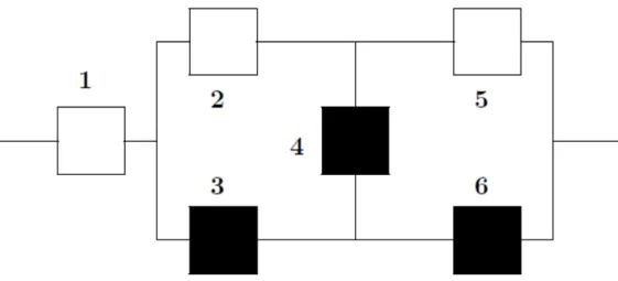
Example 1 Consider the system in Figure 1 which has been considered in Feng et al. (2016). The system has six components withK = 2types with n1 = 3 and
n2 = 3: Type 1 and type 2 components are represented respectively by blank
and black boxes. Table 1 displays the minimal survival signature of the system. Note that the minimal survival signature is computed using the relation (7) and the survival signature of the system presented in Table 1 of Feng et al. (2016).
Figure 1. System with two types of components
Using the entries in Table 1 and the equation (5), the survival function of the system can be represented as
P fT > tg
= P nT1:1(1) > t; T1:2(2) > to+ 2PnT1:2(1) > t; T1:2(2) > to 2P nT1:2(1) > t; T1:3(2) > to
+P nT1:3(1) > to 3P nT1:3(1) > t; T1:2(2) > to+ 2P nT1:3(1) > t; T1:3(2) > to: (11) Using survival copula, the survival function can be represented as
P fT > tg=Q(F1(t); F2(t));
where the distortion function is given by
Q(u1; u2) = C^(u1; u2; u2) + 2 ^C(u1; u1; u2; u2) 2 ^C(u1; u1; u2; u2; u2) + ^C(u1; u1; u1)
3 ^C(u1; u1; u1; u2; u2) + 2 ^C(u1; u1; u1; u2; u2; u2):
If the components are independent, then the distortion function becomes
Q(u1; u2) = u1u22+ 2u 2 1u 2 2 2u 2 1u 3 2+u 3 1 3u 3 1u 2 2+ 2u 3 1u 3 2:
m1 m2 (m1; m2) m1 m2 (m1; m2) 0 0 0 2 0 0 0 1 0 2 1 0 0 2 0 2 2 2 0 3 0 2 3 -2 1 0 0 3 0 1 1 1 0 3 1 0 1 2 1 3 2 -3 1 3 0 3 3 2
Table 1. Minimal survival signature of the system in Figure 1
3
Mean residual life functions
Using Theorem 1, the MRL of the system that consists of multiple types of compo-nents can be computed from
m(t) = E(T t jT > t) = n1 X m1=0 nK X mK=0 (m1; :::; mK) 1 R 0 P nT1:(1)m1 > t+x; :::; T1:(KmK) > t+xodx n1 X m1=0 nK X mK=0 (m1; :::; mK)P n T1:(1)m1 > t; :::; T1:(KmK) > t o (12):
The following result of Navarro and Hernandez (2008) is useful to examine the limiting behavior of the MRL function.
Theorem 2 (Navarro and Hernandez (2008)) LetS be a survival function such that
S(t) =
n
X
i=1
!iSi(t);
for allt 0, where S1(t); :::; Sn(t)are survival functions, and!1; :::; !n are real
numbers such that Pni=1!i = 1: Let mi(t) be MRL function corresponding to
Si(t); i= 1; :::; n;i.e. mi(t) = (Si(t)) 1 R1 t Si(u)du: If lim t!1inf m1(t) mi(t) >1; lim t!1sup m1(t) mi(t) <1;
for i= 2;3; :::; n, then the MRL function m of S satis…es
lim
t!1
m(t)
m1(t)
Because Theorem 1 presents a generalized mixture representation for a coher-ent system that consists of multiple types of dependcoher-ent componcoher-ents, Theorem 2 enables us to investigate the limiting behavior of the MRL function for such sys-tems. Application of Theorem 2 needs a multivariate distribution or survival function for modeling lifetimes of components. Suppose that the joint survival function of
T1(1); :::; Tn1(1); :::; T1(K); :::; TnK(K) is given by P nT1(1) > t(1)1 ; :::; Tn1(1) > t(1)n1; :::; T1(K) > t(1K); :::; TnK(K)> t(nKK)o = " 1 + 1 n1 X i=1 t(1)i +:::+ K nK X i=1 t(iK) # ; (13)
for t(ij) 0, i = 1; :::; nj; j = 1; :::; K; i > 0; > 0. It should be noted that the
survival copula corresponding to (13) is
^ C(u1; u2; :::; un) = h u 1 1 +u 1 2 +:::+u 1 n (n 1) i ; and P nT1(1) > t(1)1 ; :::; Tn1(1) > t(1)n1; :::; T1(K) > t(1K); :::; TnK(K)> t(nKK)o = C^(F1(t); :::; F1(t) | {z } n1 ; :::; FK(t); :::; FK(t) | {z } nK ); with Fi(t) = (1 + it) ; i= 1;2; :::; K.
In the following, we present the limiting behavior of (12) for the model (13).
Proposition 2 For the multivariate Pareto model given by (13), letC =f(i1; :::; iK) :
i1+:::+iK < j1+:::+jK and (i1; :::; iK)>0 for all j1 = 0;1; :::; n1; :::; jK =
0;1; :::; nKg: If
v1 1+:::+vK K i1 1+:::+iK K; (14)
for all (i1; :::; iK)2C; then
lim t!1 m(t) 1 1 h t+v1 1+:::1+vK Ki = 1: (15)
Proof The MRL corresponding to min(T1:(1)i1; :::; T1:(KiK)) is
1 P n T1:(1)i1 > t; :::; T1:(KiK) > t o 1 Z 0 PnT1:(1)i1 > t+x; :::; T1:(KiK) > t+xodx = 1 [1 + 1i1t+:::+ KiKt] 1 Z 0 [1 + 1i1(t+x) +:::+ KiK(t+x)] dx = 1 1 t+ 1 1i1 +:::+ KiK ;
for >1:For(v1; :::; vK)2C satisfying (14), the conditions in Theorem 2 hold
true for the MRL of min(T1:(1)v1; :::; T1:(KvK)). Thus the proof is complete.
Example 2 For the system in Figure 1, let
PnT1(1) > t(1)1 ; T2(1) > t(1)2 ; T3(1) > t3(1); T1(2) > t(2)1 ; T2(2) > t(2)2 ; T3(2) > t(2)3 o = " 1 + 1 3 X i=1 t(1)i + 2 3 X i=1 t(2)i # :
From Table 1, it is easy to see that C=f(1;2);(3;0)g. Thus from Proposition 2, if 1 2; then lim t!1 m(t) 1 1 h t+ 1 1+2 2 i = 1; and if 2 1; then lim t!1 m(t) 1 1 h t+31 1 i = 1:
It should be noted here that the limiting result in (15) depends on determination of the coe¢ cients v1; :::; vK de…ned by (14). As it is clear from Example 2, these
coe¢ cients heavily depend on the relation between the parameters 1 and 2:
Consider a coherent system that has the property that if at most r components (r < n) have failed, the system is still operating with probability 1. Then, the con-ditional expected value E(T t j Tr:n > t) represents the mean residual lifetime
function of a coherent system given that at leastn r+ 1components of the system are working at time t (Asadi and Bayramoglu (2006), Sadegh (2011)). For a coher-ent system that consists of multiple types of componcoher-ents, de…ne the following mean residual life. E(T tjT > t; Tr:n> t) = 1 Z 0 PfT > t+xjT > t; Tr:n> tgdx: (16)
For a coherent system consisting of K 2 types of components, it is easy to see that PfT > t; Tr:n> tg = X X l1+:::+lK n r+1 (l1; :::; lK)PfC1(t) = l1; :::; CK(t) = lKg = X X l1+:::+lK n r+1 (l1; :::; lK) n1 l1 ::: nK lK Sn1;:::;nK(t;l1; :::; lK); (17)
where Sn1;:::;nK(t;l1; :::; lK) is given by (5). In the following Theorem, we present the
Theorem 3 For a coherent system consisting of ni components of type i, i = 1;2; :::; K, P fT > sjT > t; Tr:n > tg = 1 P fTS > t; Tr:n> tg n1 X l1=0 nK X lK=0 X X (j1;:::;jK)2U (l1; :::; lK)N(j1; l1; n1;:::;jK; lK; nK) P n1 j1 of T(1)s t; j1 l1 of T(1)s2(t; s]; l1 of T(1)s> s; :::; nK jK of T(K)s t; jK lK of T(K)s2(t; s]; lK of T(K)s> s ; (18) whereU =f(j1; :::; jK) :j1+:::+jK n r+ 1;l1 j1 n1; :::; lK jK nKg, and N(j1; l1; n1;:::;jK; lK; nK) = n1 n1 j1; j1 l1; l1 ::: nK nK jK; jK lK; lK :
Proof By conditioning on the number of working components of each type at time
t and s; P fT > s; Tr:n > tg = n1 X l1=0 nK X lK=0 X X (j1;:::;jK)2U (l1; :::; lK) P fC1(s) = l1; :::; CK(s) =lK; C1(t) = j1; :::; CK(t) = jKg: (19)
Thus the proof follows noting that
P fC1(s) =l1; :::; CK(s) =lK; C1(t) =j1; :::; CK(t) =jKg = n1 n1 j1; j1 l1; l1 ::: nK nK jK; jK lK; lK P n1 j1 of T(1)s t; j1 l1 of T(1)s2(t; s]; l1 of T(1)s> s; :::; nK jK of T(K)s t; jK lK of T(K)s2(t; s]; lK of T(K)s> s ; for s > t and j1 l1; :::; jK lK.
In equation (19), it is quite interesting to observe that the survival signature depends on only the number of working components of each type at times(later time point) and independent ofj1; :::; jK which denote the number of working components
of each type at a previous time point t.
com-mon failure time distribution of typeicomponents is Fi(t); i= 1;2; :::; K, then P fT > sjT > t; Tr:n> tg = 1 PfT > t; Tr:n> tg n1 X l1=0 nK X lK=0 X X (j1;:::;jK)2U (l1; :::; lK) K Y i=1 ni ni ji; ji li; li Fini ji(t)(Fi(s) Fi(t))ji li(1 Fi(s))li:(20)
Corollary 3 Let r= 1 in Theorem 3. Then the conditional survival function of the system under the condition that all components are working at time t can be represented as P fT > sjT1:n> tg = 1 P nT1(1) > t; :::; Tn1(1) > t; :::; T1(K) > t; :::; Tn(KK) > t o n1 X l1=0 nK X lK=0 (l1; :::; lK) P fC1(s) =l1; :::; CK(s) =lK; C1(t) =n1; :::; CK(t) =nKg; (21) for s > t:
In the following, we obtain an expression for the joint probability involved in (18) when K = 2, i.e. the system consists of two types of components. The following result is useful since it only involves joint survival probabilities.
Proposition 3 For a system that consists of two types of components,
P fC1(s) =l1; C2(s) =l2; C1(t) = n1; C2(t) = n2g = n1 l1 n2 l2 [p1(s; t; l1; l2) p2(s; t; l1; l2) p3(s; t; l1; l2) +p4(s; t; l1; l2)]; (22) where fors > t; p1(s; t; l1; l2) = P n T1(1) > s; :::; Tl1(1) > s; Tl1(1)+1 > t; :::; Tn1(1) > t T1(2) > s; :::; Tl2(2) > s; Tl2(2)+1 > t; :::; Tn2(2) > to; (23) p2(s; t; l1; l2) = n1Xl1 i=1 ( 1)i 1 n1 l1 i P n T1(1) > s; :::; Tl1(1)+i > s; Tl1(1)+i+1 > t; :::; Tn1(1) > t T1(2) > s; :::; Tl2(2) > s; Tl2(2)+1 > t; :::; Tn2(2) > to; (24)
p3(s; t; l1; l2) = n2Xl2 i=1 ( 1)i 1 n2 l2 i P n T1(1) > s; :::; Tl1(1) > s; Tl1(1)+1 > t; :::; Tn1(1) > t T1(2) > s; :::; Tl2(2)+i > s; Tl2(2)+i+1 > t; :::; Tn2(2)> to; (25) p4(s; t; l1; l2) = n1Xl1 i=1 n2Xl2 j=1 ( 1)i+j 2 n1 l1 i n2 l2 j P n T1(1) > s; :::; Tl1(1)+i > s; Tl1(1)+i+1 > t; :::; Tn1(1) > t; T1(2) > s; :::; Tl2(2)+j > s; Tl2(2)+j+1 > t; :::; Tn2(2)> to (26) In equations (24)-(26),Pba 0if a > b. Proof Clearly, PfC1(s) = l1; C2(s) =l2; C1(t) = n1; C2(t) =n2g = n1 l1 n2 l2 PnT1(1) > s; :::; Tl1(1) > s; Tl1(1)+1 > t; :::; Tn1(1) > t Tl1(1)+1 s; :::; Tn1(1) s; T1(2) > s; :::; Tl2(2) > s; Tl2(2)+1 > t; :::; Tn2(2) > t Tl2(2)+1 s; :::; Tn2(2) so:
De…ne the events
A1 n T1(1) > s; :::; Tl1(1) > s; Tl1(1)+1 > t; :::; Tn1(1) > to A2 n T1(2) > s; :::; Tl2(2) > s; Tl2(2)+1 > t; :::; Tn2(2) > to B1 n1 [ i=l1+1 n Ti(1) > s o ,B2 n2 [ i=l2+1 n Ti(2) > s o : Then P fC1(s) =l1; C2(s) =l2; C1(t) = n1; C2(t) = n2g = n1 l1 n2 l2 [P(A1\A2) P(A1 \A2\B1) P(A1\A2\B2) +P(A1 \A2\B1\B2)]:
As it is clear from Proposition 3, to compute E(T tj T1:n > t); it is enough to
evaluate the integration in the form
1 Z
0
P nT1(1) > t+x; :::; Ta(1) > t+x; Ta(1)+1 > t; :::; Tb(1) > t;
T1(2) > t+x; :::; Tc(2)> t+x; Tc(2)+1 > t; :::; Td(2) > todx:
For the multivariate Pareto model given by (13), it can be easily seen that the later integral equals to 1 Z 0 [1 + 1((t+x)a+ (b a)t) + 2((t+x)c+ (d c)t)] dx = 1 1 [1 +t( 1b+ 2d)] 1 1a+ 2c ;
for > 1: Thus, using Proposition 3 the MRL of a coherent system when all components are functioning at timet can be computed from
E(T t j T1:n> t) = 1 [1 + 1n1t+ 2n2t] 1 ( 1) n1 X l1=0 n2 X l2=0 (l1; l2) n1 l1 n2 l2 " [1 +t( 1(n1 l1) + 2(n2 l2))]1 1l1+ 2l2 n1Xl1 i=1 ( 1)i 1 n1 l1 i [1 +t( 1(n1 l1 i) + 2(n2 l2))]1 1(l1+i) + 2l2 n2Xl2 i=1 ( 1)i 1 n2 l2 i [1 +t( 1(n1 l1) + 2(n2 l2 i))]1 1l1+ 2(l2+i) n1Xl1 i=1 n2Xl2 j=1 ( 1)i+j 2 n1 l1 i n2 l2 j [1 +t( 1(n1 l1 i) + 2(n2 l2 j))] 1 1(l1+i) + 2(l2+j) # ; (27) for >1:
Another MRL function that may be of practical interest can be de…ned as
mr1;:::;rK(t) = E(T t jT > t; Tr1(1):n1 > t; :::; TrK(K:)nK > t); (28) for 1 ri ni; i = 1; :::; K. The function de…ned by (28) represents the mean
working at time t, i= 1; :::; K: Clearly, for s > t, P T > s; Tr1(1):n1 > t; :::; TrK(K:)nK > t = n1 X l1=0 nK X lK=0 X X (j1;:::;jK)2U (l1; :::; lK) P fC1(s) = l1; :::; CK(s) =lK; C1(t) = j1; :::; CK(t) = jKg; (29)
where U = f(j1; :::; jK) : max(lm; nm rm+ 1) jm nm; m = 1; :::; Kg: On the
other hand, P T > t; Tr1(1):n1 > t; :::; TrK(K:)nK > t = n1 X l1=n1 r1+1 nK X lK=nK rK+1 (l1; :::; lK)PfC1(t) = l1; :::; CK(t) = lKg: (30)
The MRL function de…ned by (28) can be computed using (29) and (30) in
mr1;:::;rK(t) = E(T t jT > t; Tr1(1):n1 > t; :::; TrK(K:)nK > t) = 1 PnT > t; Tr1(1):n1 > t; :::; TrK(K:)nK > t o 1 Z 0 P T > t+x; Tr1(1):n1 > t; :::; TrK(K:)nK > t dx: (31)
Equation (31) corresponds toE(T tjT1:n > t) whenr1 =:::=rK = 1.
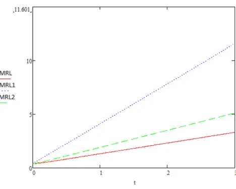
Example 1 (continued) In Figure 2, we plot m(t) = E(T t j T > t) (MRL),
m1;1(t) = E(T t j T1:n > t) (MRL1) and m2;2(t) = E(T t j T > t; T2:(1)n1 >
t; T2:(2)n2 > t) (MRL2) for the system in Figure 1 under the model (13) when
m1;1(0) =E(T) = 0:4103:
Figure 2. MRL functions of the system in Figure 1.
4
Discussion
This paper has presented general results on survival function and mean residual life for coherent systems, with multiple types of components, with the only assumption that the failure times of components of the same type are exchangeable. Hence, such components can be dependent, and also dependence of components of di¤erent types is allowed. The use of the survival signature enabled derivation of a general expression for the mean residual life for such scenarios, in particular through the introduction of the minimal survival signature for such system, generalizing this concept that was introduced by Navarro et al. (2007) for systems with a single type of components. Main future research challenges related to this work include computational issues, in particular for large real world systems, and the use of the mean residual life for decision support, where one can think about aspects like maintenance but also issues of system design.
In addition to the minimal signature, Navarro et al. (2007) also represented the survival function of a coherent system as a generalized mixture of survival functions of parallel systems and called the corresponding set of coe¢ cients as a maximal signature. This concept can be generalized to the maximal survival signature along
similar lines as the minimal survival signature presented in this paper, and may be useful for various reliability problems, e.g. stochastic comparison of two di¤erent systems.
Acknowledgments
The authors thank the Associate Editor and two reviewers for supportive and constructive comments and suggestions. This work was done while the …rst author was visiting the Durham University, Department of Mathematical Sciences with the support provided by the Scienti…c and Technological Research Council of Turkey (TUBITAK).
References
[1] M. Asadi, S. Goliforushani (2008) On the mean residual life function of coherent systems. IEEE Transactions on Reliability 57 (4), 574–580.
[2] I. Bayramoglu, M. Ozkut (2016) Mean residual life and inactivity time of a coher-ent system subjected to Marshall-Olkin type shocks.Journal of Computational and Applied Mathematics, 298, 190-200.
[3] K. Bayramoglu Kavlak (2017) Reliability and mean residual life functions of coherent systems in an active redundancy. Naval Research Logistics, 64, 19-28. [4] F.P. Coolen, T. Coolen-Maturi (2012) Generalizing the signature to systems with
multiple types of components. In: Complex systems and dependability. Springer; Berlin, p. 115–30.
[5] F.P. Coolen, T. Coolen-Maturi (2015) Modelling uncertain aspects of system dependability with survival signatures. In: Dependability problems of complex information systems. Springer; Berlin, p. 19–34
[6] S. Eryilmaz (2017) The concept of weak exchangeability and its applications, Metrika, 80, 259-271.
[7] G. Feng, E. Patelli, M. Beer and F.P.A. Coolen (2016) Imprecise system relia-bility and component importance based on survival signature. Reliarelia-bility Engi-neering & System Safety, 150, 116-125.
[8] P. Miziula, J. Navarro (2017) Sharp bounds for the reliability of systems and mixtures with ordered components. Naval Research Logistics, 64, 108-116. [9] J. Navarro (2016) Distribution-free comparisons of residual lifetimes of coherent
systems based on copula properties. Statistical Papers, DOI: 10.1007/s00362-016-0789-0.
[10] J. Navarro, S. Eryilmaz (2007) Mean residual lifetimes of consecutive-k-out-of-n
systems. Journal of Applied Probability, 44, 82-98.
[11] J. Navarro, J.M. Ruiz, C.J. Sandoval (2007) Properties of coherent systems with dependent components. Communications in Statistics-Theory and Methods, 36, 175-191.
[12] J. Navarro, P.J. Hernandez (2008) Mean residual life functions of …nite mixtures, order statistics and coherent systems. Metrika, 67, 277–298.
[13] J. Navarro, F. Spizzichino (2010) Comparisons of series and parallel systems with components sharing the same copula. Applied Stochastic Models in Business and Industry, 26, 775–791.
[14] J. Navarro, M.C. Gomis (2016) Comparisons in the mean residual life order of coherent systems with identically distributed components. Applied Stochastic Models in Business and Industry, 32, 33-47.
[15] J. Navarro, Y. del Águila, M.A. Sordo, A. Suárez-Llorens (2016) Preservation of stochastic orders under the formation of generalized distorted distributions. Applications to coherent systems, Methodology and Computing in Applied Prob-ability, 18, 529-545.
[16] J. Navarro, F. Durante (2017) Copula-based representations for the reliability of the residual lifetimes of coherent systems with dependent components. Journal of Multivariate Analysis, 158, 87-102.
[17] J. Navarro, F. Pellerey, M. Longobardi (2017). Comparison results for inactivity times of k-out-of-n and general coherent systems with dependent components. Test, 26, 822-846.
[18] E. Patelli, G. Feng, F.P.A. Coolen, T. Coolen-Maturi (2017) Simulation meth-ods for system reliability using the survival signature. Reliability Engineering & System Safety, 167, 327-337.
[19] S. Reed (2017) An e¢ cient algorithm for exact computation of system and sur-vival signatures using binary decision diagrams. Reliability Engineering & Sys-tem Safety, 165, 257-267.
[20] M.K. Sadegh (2011) A note on the mean residual life function of a coherent system with exchangeable or nonidentical components, Journal of Statistical Planning and Inference, 141, 3267-3275.
[21] F.J. Samaniego, System Signatures and Their Applications in Engineering Reli-ability. New York: Springer, 2007.
[22] F.J. Samaniego, J. Navarro (2016) On comparing coherent systems with het-erogenous components. Advances in Applied Probability, 48, 88-111.
[23] Z. Zhang, W.Q. Meeker (2013) Mixture representations of reliability in coherent systems and preservation results under double monitoring Communications in Statistics-Theory and Methods, 42, 385-397.