Control and Measuring Method for Three
Phase Induction Motor with Improved
Effi-ciency
Vom Fachbereich 18
Elektrotechnik und Informationstechnik der Technischen Universität Darmstadt zur Erlangung des akademischen Grades eines
Doktor-Ingenieurs (Dr.-Ing.) genehmigte Dissertation
von
Dipl.-Ing. Emad Ahmed Hussein Abdelkarim Geboren am 07. Oktober 1977 in Qena, Egypt.
Referent: Prof. Dr.-Ing. Peter Mutschler
Korreferent: Prof. Dr. -Ing. Ralph Kennel
Tag der Einreichung: 26.10.2010
Tag der mündlichen Prüfung: 04.02.2011
D17
Preface
This PhD thesis is the result of four years work at the Department of Power Elec-tronics and Control of Drives, Darmstadt University of Technology. Throughout this period many people contributed to my research in various ways, some directly, oth-ers indirectly related to the work presented in this thesis, but all were very helpful.
First I wish to express my gratitude to Prof. Dr.-Ing. Peter Mutschler, my supervi-sor, for his guidance, encouragement, inspiration, and valuable arrangements during this research. I greatly appreciate his patience in scrutinizing this thesis. His pains-taking efforts and competence guidance helped me through out my project. His keen interest boosted my motivation further and encouraged me for making my work a successful.
I would sincerely thank Prof. Dr.-Ing. Ralph Kennel for his interest and for acting as co-advisor.
I thank Darmstadt University of Technology (TUD) for financially supporting and buying the required equipments and devices for my work.
I would also thank Cultural Bureau and Educational Mission, Embassy of Egypt in Berlin for providing financial support during these years.
I would like to thank all my colleagues and secretary at the Department of Power Electronics and Control of Drives, for their support and comments, provided me with valuable suggestions and discussions.
I would also like to thank the workshop staff for providing me their invaluable work experiences in workshop especially while I was building the system.
I would like to avail this opportunity to express my heartiest gratitude to my wife for her encouragement, support during my study and our residence in Germany.
Abstract
Abstract
This thesis deals with improving and measuring the efficiency of variable speed induction motor drives. Optimized efficiency is achieved by adapting the magnetizing level in the motor according to the load percentage.
The thesis investigates on the efficiency improvement of squirrel cage induction motors fed by SVM-VSI, by using the loss model method.
A new expression for the optimal air gap flux is calculated from a detailed loss model. This loss model comprises the copper loss, iron loss, friction, windage, stray, and harmonic loss. The calculated optimal air gap flux is a function of these losses and also considers the non-linearity of the magnetizing inductance and the effect of the temperature on the motor parameters (stator and rotor resistances).
The proposed loss model improves the efficiency of a speed sensorless indirect field oriented control (IFOC) induction motor.
The (IFOC) of an induction motor is sensitive to motor parameter variation. Rotor and stator resistances vary with the motor temperature, and the proposed loss model controller depends on the motor parameters. So an on-line estimation of motor pa-rameters using parameter adaptive observer is used.
An on-line search control method shows the accuracy of the optimal flux values, which are calculated by using the proposed loss model.
By using the calculated optimal air gap flux for speed sensorless indirect vector controlled induction motor, an improvement in motor efficiency and power factor are achieved especially at light load.
If there is an increase in the load while the motor is operating with the optimal flux value, the flux will be right away increased to the rated value, and later, the suitable optimal flux value according to the new load torque is calculated.
Measuring the efficiency of the induction motor according to IEEE-112B standard requires highly accurate measuring devices, where the inaccuracy of the power me-ter and torque meme-ter should not exceed (0.1%), and (1 RPM) for speed sensor. But such devices are expensive.
An accurate system using a FPGA was designed to calculate the motor efficiency without requiring a power meter. By adapting the motor voltages and currents sig-nals, load torque meter signal, and position sensor signal the average electrical and mechanical motor powers are calculated in a FPGA. The accuracy of the calculated electrical power is verified by using advanced power meter (with accuracy equals 0.1%), in order to satisfy the recommendation of the standard IEEE-112B.
Fuzzy Logic Controller improves the motor speed performance when compare to PI speed controller.
The improvement in the efficiency, the power factor and the motor stability under fast load variations by using the proposed optimal flux control method is compared with the rated flux control method experimentally.
Also, the experimental results show the accuracy of the designed efficiency meas-uring system.
Kurzfassung
Diese Arbeit beschäftigt sich mit Effizienzsteigerungen und der Messung von drehzahlgeregelten Induktionsmotoren. Optimierte Effizienz wird durch die Anpas-sung des Magnetisierungsstroms in dem Motor je nach der Belastung erreicht.
Die Arbeit untersucht die Verbesserung der Effizienz von Käfigläufer-Asynchronmotoren am U-Umrichter mit der Verlust Model-Methode.
Eine neue Beziehung für den optimalen Luftspaltfluss wird durch ein detailliertes Verlustmodell hergeleitet, bei dem Kupfer Verluste, Eisen-Verluste, Reibung, Ventila-tionsverluste, und harmonische Streu-Verluste, als Funktion des Luftspaltflusses be-rechnet werden. Dabei wird die Nichtlinearität der Magnetisierungs-Induktivität und die Wirkung der Temperatur auf die Motorparameter (Stator und Rotor Widerstände) berücksichtigt. Das vorgeschlagene Verlust-Modell wird verwendet, um die Effizienz der sensorlosen indirekten feldorientierten Regelung zu verbessern (IFOC). Die IFOC einer Asynchronmaschine ist empfindlich gegenüber Motorparametervaria-tionen vor allem, Rotor und Stator Widerständen variieren mit der Motortemperatur. Da die vorgeschlagene Methode von den Motor-Parametern abhängt, wird eine Onli-ne-Schätzung der Motor-Parameter mit Hilfe eines Parameter adaptiven Beobachters eingesetzt.
Ein Online-Suche Verfahren zeigt die Genauigkeit des berechneten optimalen Fluss-Wertes mit Hilfe des vorgeschlagenen Modells.
Vor allem im Teillastbereich wird durch die Verwendung des berechneten optima-len Luftspaltflusses bei den sensorlosen indirekten drehzahlgeregelten Induktionsmo-toren eine Verbesserung des Wirkungsgrades und Leistungsfaktors erreicht.
Bei einer Erhöhung des Lastmomentes und damit einhergehendem Geschwindig-keitsabfall wird zunächst Nennfluss vorgeben und anschließend der zum neuen Be-triebspunkt passende optimale Fluss-Sollwert berechnet.
Die Messung der Effizienz der Asynchronmaschine nach dem Standard IEEE-112B erfordert hochpräzise Messgeräte, bei denen der Messfehler 0,1% nicht über-schreitet. Aber solche Geräte sind teuer.
Ein genaues System mit einem FPGA wurde entwickelt, um den Wirkungsgrad des Motors zu bestimmen. Durch die Erfassung der Motor Spannungen und Ströme, des Lastmoments und der Position kann in einem FPGA die elektrische Eingangs-leistung und die mechanisch abgegebene Leistung berechnet werden. Die berechne-te elektrische Leistung wird unberechne-ter Verwendung eines käuflichen Leistungsmessers (0,1%) geprüft, um die Empfehlungen nach dem Norm IEEE-112B zu erfüllen.
Fuzzy-Logik-Regler verbessert die Regelgüte der Drehzahl des Motors im Ver-gleich zum PI-Regler.
Die Verbesserung der Effizienz, des Leistungsfaktors und der Stabilität bei schnel-len Lastschwankungen wird experimentell gezeigt.
Auch zeigen die experimentellen Ergebnisse die Richtigkeit des ausgelegten Messsystems.
I
Contents
1. INTRODUCTION ...1
1.1. Advantages of the Induction motor...1
1.1.1. Induction motor common loads...1
1.1.2. Induction motor control methods ...1
1.2. Induction motor efficiency...1
1.2.1. Simple state control ...4
1.2.2. Loss model based control...4
1.2.3. Search control method...8
1.3. Formulation of the problem...11
1.4. Structure of the thesis...11
2. THE PROPOSED LOSS MODEL BASED CONTROLLER AND EFFICIENCY DETERMINATION METHOD ...12
2.1. Induction motor losses...12
2.1.1. Stator copper loss...12
2.1.2. Rotor copper loss...12
2.1.3. Core loss...13
2.1.4. Friction and windage losses ...13
2.1.5. Stray loss ...13
2.1.6. Harmonic losses ...14
2.2. Temperature and skin effect...14
2.3. Non-linearity of the magnetizing current...15
2.4. The proposed loss model ...15
2.4.1. Induction motor variables...15
2.4.2. Optimal air gap flux calculation...16
2.5. Implementation of the proposed loss model ...18
2.5.1. FOC block diagram...19
2.5.1.1. PI current controller ...20
2.5.2. Speed estimation ...21
2.5.3. Parameters estimation...23
2.5.4. Motor stability...27
2.6. Determination of the efficiency ...29
2.6.1. The proposed measuring method...29
2.6.2. The proposed sampling for efficiency determination ...30
2.6.3. Electrical and mechanical powers calculation ...30
3. EXPERIMENTAL SET-UP ...32
3.1. The motor ...32
3.1.1. Coupling and load...32
3.2. Inverter board ...32
3.2.1. IPM evaluation board...34
3.2.2.1. Calculation of the ripple current induced from the rectification ...35
3.2.2.2. Calculation of the ripple current from the inverter side ...37
3.2.2.3. Choosing the capacitor ...41
3.2.3. Diode bridge rectifier...41
3.2.4. Optocouplers ...42
3.2.5. Current sensors ...42
3.2.6. Heat sink...42
3.2.7. Overall Inverter board design ...42
3.3. Inverter interface board ...43
3.4. Computer interface board...44
3.5. Efficiency determination system ...45
3.5.1. Analog signal conditioning board...46
3.5.2. Sensor to Digital code...46
3.5.2.1. Analog to digital conversion...46
3.5.2.2. Multiplexer selector inputs signals ...48
3.5.2.3. Digital Output ...49
3.5.2.4. Electrical power calculation ...49
3.5.2.5. Mechanical power calculation...50
3.5.2.6. Sensor to Digital BUS Control ...51
3.5.3. Interrupt service routine ...52
3.5.4. Testing the system...53
4. IFOC OF INDUCTION MOTOR BASED ON THE PROPOSED LOSS MODEL ...55
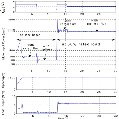
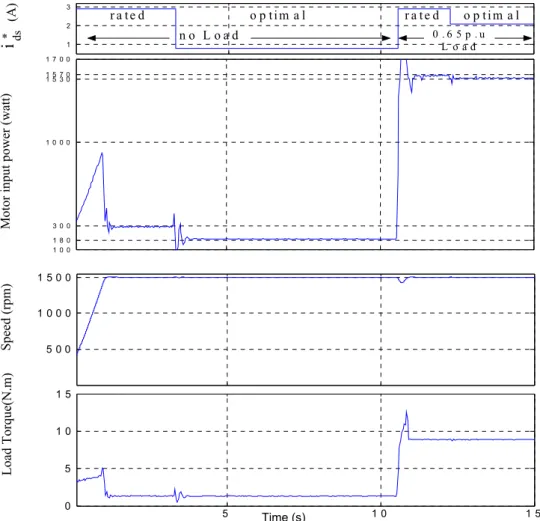
4.1. Efficiency improvement using the proposed loss model...55
4.2. The accuracy of the designed measurement system ...60
4.3. Motor oscillation...61
4.4. Proposed loss model controller via on-line search controller ...63
4.4.1. Search control...64
4.4.2. Accuracy of the proposed loss model controller ...65
4.5. Conclusion...66
5. FUZZY LOGIC CONTROLLER...68
5.1. Why fuzzy logic speed controller? ...68
5.2. Fuzzy sets and fuzzy logic...69
5.3. Membership functions ...70
5.4. Fuzzy control system...70
5.4.1. Fuzzification module (fuzzifier) ...71
5.4.2. Rule base...71
5.4.3. Interface engine ...71
5.4.4. Defuzzification ...72
5.5. Fuzzy speed control system ...73
III 6. CONCLUSION ...78 6.1. Summary ...78 6.2. Future work...80 BIBLIOGRAPHY ...81 APPENDIX ...85
A.1 Kioskardis and Margaris loss model controller...85
A.2 G. Joksimovic´ and A. Binder loss model...86
A.3 The tested induction motor parameters...87
A.4 Optimal air gap flux equation...87
A.5 Experimental set-up photo ...89
List of symbols
fw
C :Friction and windage constant.
str
C :Stray loss constant.
c
i :Capacitor current.
ds
i :Flux producing current component.
* ds
i :Reference flux producing current component.
inv
i :Inverter current.
inv,ac
i :AC component of the inverter current.
qs
i :Torque producing current component.
* qs
i :Reference torque producing current component.
rec
i :Rectifier current.
rec,ac
i :AC component of the rectifier current.
inv,ac,RMS
I :The ripple current resulting from the inverter side (RMS).
r
I :Rotor current.
rec,ac,RMS
I :The ripple current resulting from the rectifier side (RMS).
s
I :Stator current.
e
k :Eddy current coefficient given by material and design of the motor.
h
k :Hysteresis coefficient given by material and design of the motor.
m
L :Magnetizing inductance.
r
l :Rotor leakage inductance.
r
L :Rotor self inductance.
s
l :Stator leakage inductance.
s
L :Stator self inductance.
P :Pole pairs.
cu,r
P :Rotor copper loss.
cu,s
P :Stator copper loss.
dc
P :DC link power.
e
P :Eddy current loss.
fw
P :Friction and windage power loss.
h
P :Harmonic power loss.
h
P :Hysteresis loss.
iro n
P :Iron loss.
lo s s
P :Motor total loss.
loss,d
P :Motor total loss in d-axis.
loss,q
P :Motor total loss in q-axis.
r
P :Rated power.
str
P :Stray power loss.
r
R :Rotor resistance.
s
V
vsr
R :Sharing resistance.
s :Slip.
T :Electro magnetic torque.
Tc :The discharge time.
Ts :Sampling time.
Udc :DC link voltage.
αs
V ,Vβs :Stator voltage vector.
k
β :The angular position of the rotor flux linkage.
µ :Degree of Membership.
e
θ :The angular position of the rotor flux linkage.
φ :Flux linkage.
opt.
φ :Optimal air gap flux.
αr
φ ,φβr :Stationary rotor flux components in αβaxes.
αs
φ ,φβs :Stationary stator flux components in αβaxes.
ω,ωr :Motor angular speed.
e P ωr
ω = ∗ :Angular rotor frequency.
s
Abbreviations
ADDR :Address/Data.
ASC :Analog Signal Conditioning.
A/D :Analog-to-Digital.
BJT :Bipolar Junction Transistor.
CLK :Clock.
COA :Center Of Area.
DC :Direct Current.
EMF :Electro Motive Force.
FLC :Fuzzy Logic Controller.
FO :Fault Output.
FOC :Field Oriented Control.
FPGA :Field Programmable Gate Array.
GTO :Gate Turn-off Thyristor.
Gi :Current gain.
GT :Torque gain.
Gv :Voltage gain.
IFOC :Indirect Field Oriented Control.
IGBT :Insulated Gate Bipolar Transistor.
IM :Induction Motor.
IPM :Intelligent Power Module.
LMC :Loss Model Controller.
m :Modulation Index.
MF :Membership Function.
MIMO :Multi-Input-Multi-Output.
NN :Neural Network.
PCI1 :Computer Interface Board 1.
PCI2 :Computer Interface Board 2.
PI :Proportional Integral.
PWM :Pulse Width Modulation.
RD :Read.
RPM :Revolution Per Minute.
RTAI :Real Time Application Interface.
S2D :Sensor to Digital.
SC :Search Controller.
SCR :Silicon-Controlled Rectifier.
SISO :Single-Input-Single-Output.
SVM :Space Vector Modulation.
VSD :Variable Speed Drive.
VSI :Voltage Source Inverter.
VVFF :Variable Voltage Fixed Frequency.
VVVF :Variable Voltage Variable Frequency.
1.1 Advantages of the Induction motor 1
1. Introduction
1.1. Advantages of the Induction motor
Induction motor is a simple and wide used electromechanical energy conversion mean. It is the commonly used motor in industry, more than 50% of the electrical en-ergy is consumed by induction motors because of their advantages.
The squirrel-cage induction motor is cheap. No slip ring and brushes are used as in the case of ac synchronous motor or commutator and brushes as in the case of dc motor.
The motor design is simple and it is safely used in harsh environments. It is rug-ged because of lack of wiring in the rotor, and maintenance free. It has direct line start ability, and can withstand heavy overload for long time.
1.1.1. Induction motor common loads
The groups of applications that are often used in connection with induction motors are classified according to their mechanical characteristics and control requirement.
With respect to mechanical characteristics (torque versus speed) loads are di-vided to three groups:
1-constant torque characteristic, for load with speed varies in narrow ranges, such as conveyors.
2-progressive torque characteristic, for most loads with a widely varying speed, typical for pumps, fans, blowers, compressors, and electric vehicles.
3-regressive torque characteristic, typical for winders, there with a constant ten-sion and linear speed of the wound tape, an increase in the coil radius is accompa-nied with a decreasing speed and an increasing torque.
The type and the accuracy of the used controller depend on the application of the drive. In pumps, blowers, fans, and conveyors the main controlled variable is the load speed. For these loads high control accuracy is not necessary compared with the winders and electric vehicles, which require high control quality.
In elevator drives and machines tools the controlled variable is the position; the designed controller should have a high dynamic performance.
1.1.2. Induction motor control methods
The advent of power electronic converters with forced commutation in 1960s and later with turn-off power semiconductors (BJT, GTO, and IGBT) made possible the use of the induction motor as a variable speed drive (VSD).
Researchers at Siemens and Darmstadt University of Technology (Hasse, Jötten) developed the theory of field-oriented control in 1968-1969. Since this date, re-searchers all over the world have implemented many accurate practical control algo-rithms depending on this theory.
As shown in Figure 1.1, two approaches to control the induction motor are: - 1) Scalar control where magnitudes of the stator voltages and the stator fre-quency are the controlled components.
2) Vector control approach uses the space vector model of the induction motor to precisely control the torque both in steady state and transient operation.
1.2. Induction motor efficiency
Due to their low price and reliability induction motors are widely used in the indus-try. The electricity bill for a motor for some months may be more than its cost, there-fore, even small efficiency improvement will produce notable cost saving.
maintain the motor efficiency at high level compared with the mechanical solution of using adjustable nozzle in application such as pumps and fans.
The speed and the torque of an AC electric motor can be controlled by varying the frequency and voltage of the electricity supplied to the motor. This control replaces inefficient energy robbing speed control methods which may use belts and pulleys, throttle valves, fan dampers and magnetic clutches.
By using variable speed drives (VSDs) the following benefits are obtained: -
• VSDs advantages
Gentle startups and gradual slowdowns reduce motor stress. Small size makes them ideal for usage.
Energy savings are up to 20 percent [30].
• VSDs and Versatility
VSDs save energy in pumping applications such as in municipal water systems, chemical and petrochemical industries, pulp and paper industries and food indus-tries. They also save energy when applied to air handling and ventilation systems. VSDs provide precise and efficient speed control in conveyor systems used in the food, paper, automotive and consumer goods industries. They are also used in crushers, grinding mills, rotary kilns, presses, rolling mills and textile machinery.
In d u c tio n m o to r c o n tr o l s tr a tig ie s S c a la r c o n tro l V e c to r c o n tro l O p e n lo o p W ith s p e e d s e n s o r S e n s o r le s s S e n s o r le s s W ith s p e e d s e n s o r D ir e c t to r q u e c o n tr o l F ie ld o r ie n te d v e c to r c o n tro l S ta to r - o r ie n te d v e c to r c o n tr o l R o to r -o r ie n te d v e c to r c o n tr o l A ir g a p -o r ie n te dv e c to r c o n tr o l In d ir e c t D ir e c t D ir e c t In d ir e c t D ir e c t In d ir e c t N a tu ra l fie ld o r ie n ta tio n
1.2 Induction motor efficiency 3
Improving the efficiency of the induction motor can be done by two ways.
1. by improving the motor design (efficient motors): -
The efficiency of the motor can be improved from three to eight percent [30]. Heavier copper wire, higher core-steel grade, thinner core laminations, better bear-ings and reduced windage design add up to better efficiency. Even though initial cost is higher, payback can be very short, especially for motors that are in permanent use. The action that can be taken to reduce the induction motor losses, given a con-stant core volume [1] is shown in TableI.
Table I. Reduction of the induction motor losses
Loss Possible design
changes
Positive effect on losses Adverse effects
Stator copper loss
1. Increase the copper fill factor.
2. Increase stator slot size and amount of copper wire in slot. 3. Decrease length of coil extensions.
1. Decrease stator resis-tance.
2. Decrease stator resis-tance.
3. Decrease stator resis-tance.
1. Increase cost and difficult to build.
2. Increase cost and difficult to build.
3. Possible increase of inrush current- difficult to build. Core loss (hysteresis and eddy current loss) 1. Change to lami-nated steel. 2. Decrease lamina-tion steel thickness.
3. Improve core plat-ing/ annealing proc-esses.
1. Decrease hysteresis loss.
2. Decrease eddy current loss.
3. Decrease eddy current loss.
1. Increase cost and reduce availability of the materials.
2. Increase cost and reduce availability of the materials.
3. Increase cost and use of energy.
Rotor cop-per loss
1. Increase flux den-sity in the air gap.
2. Increase rotor bar size.
3. Increase end-ring size.
4. Increase rotor bar / end ring conductivity.
1. Decrease in slip and rotor copper loss.
2. Decrease in rotor cop-per loss.
3. Decrease in rotor cop-per loss.
4. Increase rotor bar / end ring conductivity.
1. Increase in inrush current.
2. Maybe higher inrush current and decrease starting torque. 3. Same as no.2. 4. Same as no.2. Windage and fric-tion loss
1. Optimize fan de-sign.
2. Optimize bearing selection.
1. Reduce operating tem-perature.
2. Reduce friction loss.
1. Can cause increase in noise levels.
2. May affect noise level or impose speed or bearing loading re-striction.
Stray load loss
1. Insulate rotor bars.
2. Increase air gap.
3. Eliminate rotor skew.
1. Reduce bar to lamina-tion currents.
2. Reduce high frequency surface losses.
3. Reduce the rotor cop-per loss.
1. Increase cost.
2. Reduce power factor.
3. Increase torque rip-ple and noise levels.
2. by introducing control strategies based on optimal air gap flux, which reduce the motor losses for the already working motors. There are three main categories as fol-lows.
1.2.1. Simple state control
In 1977 Nola [2] optimized the efficiency of an induction motor by using variable voltage fixed frequency (VVFF) converter. He found that by controlling triac fire an-gle, the fundamental stator voltage and then the efficiency are controlled.
In [3], an optimal efficiency control for AC motor by thyristor voltage controller was implemented. As shown in Figure 1.2, by controlling thyristors fire angles of soft start converter, the motor efficiency can be controlled. The efficiency of a lightly loaded in-duction motor can be substantially improved by controlling the voltage applied to it. In addition, controlling the voltage also improves the power factor at which the motor operates.
As the power transistor developed, the topology of using variable voltage variable frequency (VVVF) was spread, and the PWM-VSI with line side diode rectifier is used in most variable speed drives until today.
Improving the induction motor efficiency by controlling the power factor was used in [4], [5], and [6]. This controller does not require speed information, but the obsta-cles are in the way to measure the power factor and generating reference values.
In [4], the constant power factor controller does not result in an optimally controlled motor, and algorithms which minimize power factor angle or stator power appear to have substantial benefits over the constant power factor controller.
Calculating and saving the optimal slip frequency in a look-up table versus the mo-tor speed was proposed by [7], where the momo-tor terminal voltage is controlled accord-ing to the reference slip.
1.2.2. Loss model based control
In this category, the optimal motor efficiency relies on the calculation of the total motor losses.
The accuracy of the loss model controller (LMC) depends on the correct modeling and parameterization of the motor losses. Margaris and Kioskardis [8] calculated the optimal flux at steady state, as a function of the stator current; see equation (1.1). The derivation of equation (1.1) is shown in Appendix A.1.
2 2 r s opt. s s 2 2 r ps 1+ω T =Ι G 1+ω T φ 1.1 where φopt.: optimal air gap flux
Ιs : stator current
ωr : motor angular speed
I.M
1.2 Induction motor efficiency 5 L s r s m L s C R +R G =X 2c R R ′ ′ + T s str L s r C C R R = ′ + 2 e L m str ps 2 h L m 2(k c X +c ) T = k c X
But this model does not include the saturation effect and harmonic loss (disadvan-tages).
In [9], Garcia proposed maximizing the IM efficiency by the optimum balance be-tween copper and iron losses. This balance can be obtained by controlling the induc-tion motor magnetic flux. The task can be carried out by a field-oriented scheme. For a given speed and torque, he calculated the flux producing current component (ids) as
function of torque producing current component (iqs) , as follows:
i
ds=
k i
min qs where(
)
(
)
s qls r qls r min 2 2 s qls r m R R R R R k R R R L + + =+ + ω ,
R
qlsis the stator iron loss resistance in q-axis. In this model, there are some simplifications like- The stator and rotor leakage inductances (Llsand Llr)were neglected.
- The resistances that represent the rotor iron losses were considered as a part of the rotor resistance.
- Ignoring effects such as magnetic saturation and temperature. - Neglecting the stray loss.
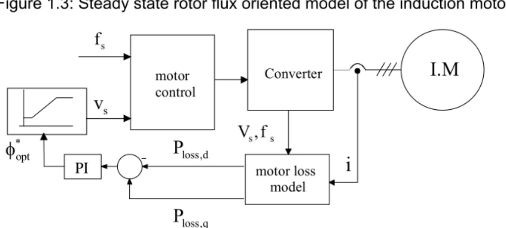
By Flemming and B. Thoegersen [10, 15] the optimal efficiency point is found by equalizing the losses related to the torque producing current component with the losses related with the flux producing current component. The used motor model is shown in Figure 1.3. This model is the steady state case of the transient rotor-flux ori-ented motor model. From this model, the total motor loss in steady state is equal the sum of the following three components:
(
)
2(
)
2 s m s 2 loss,d s s m 2 sd Fe Fe L R P R L i R R ⎛ ω ⎞ ⎜ ⎟ = + + ω ⎜ ⎟ ⎝ ⎠(
)
2 loss,q r s sq P = R +R i s loss,dq s m sd sq Fe R P 2 L i i R = − ωThe developed electro-magnetic torque is
m sd sq T PL i i= Assuming, sq sd
i
A
i
=
,by representing
i
sd, andi
sq as function of electro magnetic torque and variable A, the total motor loss becomesloss loss,d loss,q loss,dq
=
(
)
(
)
(
)
2 2 s m s s s s m 2 s r s m m Fe Fe Fe L R R T 1 R L R R A 2 L PL R R A R ⎡⎡ ω ⎤ ⎤ ⎢⎢ + + ω ⎥ + + − ω ⎥ ⎢⎢⎣ ⎥⎦ ⎥ ⎣ ⎦For constant torque, the minimum loss was found by differentiating the total motor loss with respect to A.
The criterion to cause minimum loss is by equating Ploss,dandPloss,q.
loss,d loss,q
P =P
It was proposed to solve this equation with a PI-controller as shown in Figure 1.4. But it was not clear, how the coefficients of the PI controller were calculated. Addi-tionally it was assumed that the model parameters are constant, which is not true, because the magnetizing inductance and the core loss resistance depend on the flux level.
There is always a tradeoff between accuracy and complexity of the developed LMC. In [11], a simple LMC was suggested by neglecting the stray, friction, and har-monic losses. An induction motor model in d-q coordinates is referenced to the rotor magnetizing current. This transformation results in no leakage inductance on the ro-tor side, and it was used in deriving the moro-tor loss model in steady state (see Figure 1.5). The total loss was given by:
loss cu,s iron cu,r P =P +P +P
2 2 2 2
s sd sq fe sq r r r R (i i ) R (i′ i ) R i′
= + + − +
Then the optimal ids is found by deriving this equation with respect to ids and equating
to zero.
loss ds dP
di =0
This method implies that the minimum total power loss in the motor is when the d and q axes losses are equal. In addition, the optimum level of the magnetizing cur-rent is given by:
I.M s s V ,f motor control s f s v
i
motor loss model * opt φ PI loss,d P loss,q P ConverterFigure 1.4: Scheme for energy optimal model based control.
s v s
i
R s ls lm RF e Rr /S idsi
qs iFe ir1.2 Induction motor efficiency 7 mr _ opt. sq i =ki , q d R k R = where 2 2 m d s r fe r L R R R R ′ = + ω ′ + ′ , q s fe fe r R R R R R R ′ ′ = + ′ + ′
Although the LMC is cheap and faster, it is sensitive to the loss model inaccura-cies, and parameters variation. In [12] G. Joksimovic´, A. Binder calculated the additional losses, at no load, in a high-speed squirrel cage induction motor fed from sinusoidal and inverter supplies.
The additional no load losses in case of sinusoidal supply are due to the space harmonics and flux pulsations in rotor teeth. In case of using the inverter supply, there is increase in the losses due to the voltage harmonics. This harmonics pro-duce additional high-frequency stator current components, which may cause first-order skin effect losses in the parallel copper wires of the stator coils and second-order skin effect in the conductors, (see Figure 1.6).
Figure 1.6: Measured iron losses and no-load additional losses at sinusoidal and inverter supply vs. fundamental stator frequency [12].
s R m L′ ds u s e qs L′ ωi mr
i
dsi
s R fe R′ qs u s e ds L′ ωi fei
qsi
r R′ ri
(a) (b)The calculation of the motor losses for reference [12] was inserted in Appendix A.2. This model is accurate, but it needs information about the mechanical design of the motor, which is not usually available for all the motors.
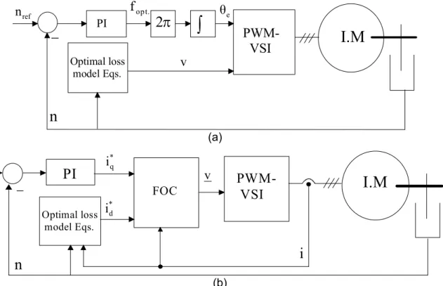
Figure 1.7 shows in general the block diagram of the loss model based controller for scalar and vector controlled induction motor.
1.2.3. Search control method
In a search controller (SC), the motor input power is measured, and one physical quantity such as air gap flux or stator current or DC current is varied till the minimum input power is detected for a given load torque and speed [13-21].
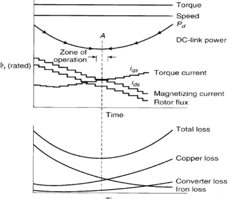
The motor losses and their variation with reducing the flux for constant load torque and constant speed is shown in Figure 1.8. With reducing the flux from rated value, the motor copper loss increases, and the core loss decreases. The total loss de-creases to a minimum value and then inde-creases.
The principle was first mentioned in [14]. He proposed to start the drive with a rated V/f ratio. When a constant torque demand is detected, the V/f ratio is reduced until the minimum DC link current is detected [15].
In [16] assumed that the machine operates initially at rated flux in steady state with low load torque at certain speed, as shown in Figure 1.8. The rotor flux is reduced in steps by reducing the flux forming current component ids, this results in an increase of
the torque forming current component iqs. So, the developed torque remains
con-stant. It is noticed that the core loss decreases with a decrease of the flux and the copper loss increases, but the total losses (motor and converter loss) decrease im-proving the overall efficiency. This is reflected in the decrease of the DC link power for the same output power. The search is continued until the system settles at the minimum DC link power (i.e., maximum efficiency) point A; any search attempt after point A adversely affects the efficiency and forces the search direction towards the point A. PI VSI
I.M
Optimal loss model Eqs. ref nn
− v opt. f e θ2
π
∫
(a)PI
VSII.M
Optimal loss model Eqs. refn
n
− FOC v * q i * d ii
(b)1.2 Induction motor efficiency 9
In [17], a minimization of stator current by search control instead of minimization of input power is derived.
Figure 1.9 shows the use of the search control for scalar and vector controlled induction motor.
The drawbacks of the search controller are:
Figure 1.8: Loss variation of Induction motor with flux decreasing for constant speed and constant load torque [16].
PI VSI I.M n −
v
s f V/f eθ
2
π
∫
z-1 ref nn
Input power measurment Low pass filter P k P k-1 − − −∫
every 50ms (a) z-1 I.M ref n n − * FOC d i VSI Input power measurment v * q i Low pass filter P k P k-1 − − −∫
PI every 50ms (b)1) slow convergence and torque variations
2) extra hardware for measuring motor input power
In [18], fuzzy logic controller was used instead of classic search control algorithm to make the algorithm convergence faster, as shown in Figure 1.10.
In this model, the DC link power P (k)dc is compared with the previous value to de-termine the decrement (or increment)ΔP (k)dc . Based on the input signals, the decre-ment step Δi (p.u)dc is generated from the fuzzy interface system.
Instead of fuzzy logic controller, a neural network (NN) was used in the search control [22-24]. The NN structure is as shown in Figure 1.11. The model has one in-put layer, one hidden layer, and one outin-put layer. The inin-put layer includes two neu-rons to which the rotor speed and electromagnetic torque are connected as inputs to network. The output layer has only one neuron for the magnetizing current ids.
A hybrid method is proposed in [25-27], using a LMC and SC where the first esti-mation is from the LMC and the subsequent adjustment of the flux is through the SC.
PI
I.M
ref n n − FOC * q i * d i VSI DClink power measurment v∑
* d i Δ n n Δ dc P fuzzy efficiency controllerFuzzy Efficiency Controller
scaling factor computation n Δ dc P (k) Δ dc P (p.u.) Δ b ase P Ib ase * ds i (p.u.) Δ
Δ
i
*ds n dc P (k) * qs i 1 z− 1 z− dc P (k 1) Δ −÷
Fuzzy interference anddefuzzy-ficationFigure 1.10: Search control using fuzzy logic controller.
r ω
T
ds i
input layer hidden layer output layer
1.3 Formulation of the problem 11
1.3. Formulation of the problem
Induction motors are large consumers of the electric energy, and many of them are not working all the time with their rated load torque. A significant improvement in the motor efficiency at partial loads can be achieved by using different control strate-gies.
In industry, improving the efficiency for already working induction motors using search control method is not preferred for economic reason like requirement of the additional hardware.
So, at first the thesis focuses on the efficiency improvement of squirrel cage induc-tion motors fed by SVM-VSI using the loss model based method.
A new expression for the optimal air gap flux is calculated from a detailed loss model. This loss model comprises the copper loss, iron loss, friction, windage, stray, and harmonic loss. The calculated optimal air gap flux is a function of these losses and also considers the non-linearity of the magnetizing inductance and the effect of the temperature on the motor parameters (stator and rotor resistances).
Secondary,Measuring the efficiency of the induction motor according to IEEE-112B standard requires highly accurate measuring devices, where the inaccuracy of the power meter and torque meter should not exceed (0.1%), and (1 RPM) for speed sensor. But such devices are expensive. To reduce the measurement cost, an accu-rate system using a FPGA was designed to calculate the motor efficiency without re-quiring a power meter.
1.4. Structure of the thesis
The thesis is divided into six chapters.
Chapter two explains in detail the proposed loss model based controller and its implementation. The proposed loss model is used to improve the efficiency of a speed sensorless IFOC induction motor. The speed estimation, the stator and the ro-tor resistances estimation, and the moro-tor stability are discussed. Also, it explains the proposed economic and accurate method to determine the motor efficiency.
Chapter three presents the experimental set-up, the design of the accurate effi-ciency measurement system and comparison with an accurate power meter which has an accuracy of 0.1%. An economic inverter board was designed using an intelli-gent power module (IPM from Mitsubishi). Selection and design of the suitable DC link capacitor, current measurement sensor and heat sink are discussed in details.
Chapter four clarifies experimentally the advantages of the proposed loss model in efficiency and power factor improvements. An on-line search control method is used to examine the accuracy of the calculated optimal flux values by the proposed loss model.
Chapter five illustrates an improvement of a motor speed response, where the speed response can be improved by using a PI Fuzzy Logic speed controller instead of a conventional PI speed controller.
2. The proposed loss model based controller and
effi-ciency determination method
This chapter explains the proposed loss model based controller, and an accurate and economic measuring method for motor efficiency determination.
In the proposed model, the motor electrical and mechanical losses are repre-sented as function of the air gap flux. An on-line estimation for stator and rotor tances is used to consider the effect of temperature and skin effect on winding resis-tances. Additionally, the non-linearity of the magnetizing current is included.
This model uses an off-line calculated look-up table where the optimal flux values are stored for different motor load torques and different required speeds.
The efficiency is determined from the calculated average electrical power and av-erage mechanical power by FPGA. The electrical power is calculated by measuring and adapting two line-to-line voltages and two line currents instead of using power meter with accuracy equal 0.1% to fulfill IEEE 112B standard recommendation [29]. The average mechanical power is calculated from the measured load torque meter and speed sensor signals.
2.1. Induction motor losses
The losses are classified as fundamental frequency losses and harmonic losses. The fundamental frequency losses consist of stator and rotor copper losses, core losses (eddy current and hysteresis), stray losses, and mechanical losses (friction and windage).
The electrical losses are represented as shown in Figure 2.1 by the stator, the ro-tor, the stray, and core resistances.
2.1.1. Stator copper loss
The stator copper loss is calculated as
2 cu,s s s
P =3I R
2.1where Pcu,s : stator copper loss Rs : stator resistance Is : stator current 2.1.2. Rotor copper loss
The rotor copper loss is calculated as
2 cu,r r r
P =3I R 2.2 where Pcu,r : rotor copper loss
Rstr Rs
X
mR
m XsR
r/s
Xr EV
ISI
m Ir2.1 Induction motor losses 13 Rr : rotor resistance
Ir : rotor current
Temperature and influence of skin effect of the winding would be necessary for a correct copper losses calculation. To circumvent this, the stator and rotor resistances are estimated on-line by using adaptive motor parameter observer [28].
2.1.3. Core loss
Energy lost by changing the magnetization of the steel laminations. Losses are due to eddy currents and hysteresis. From Steinmetz expressions for core losses, the hysteresis and eddy current losses in case of sinusoidal flux distribution are as follows. 2 h h s P =k φ ω 2.3 2 2 e e s P =k φ ω 2.4 where Ph : hysteresis loss
Pe : eddy current loss
kh : hysteresis coefficient given by material and design of the motor
ke : eddy current coefficient given by material and design of the motor φ : flux linkage
ωs: angular stator frequency So the stator core loss is
2 2 2
s,c o re s,h s s,e s
P = k φ ω + k φ ω
The rotor core loss is the same as stator core loss but with slip frequency instead of stator frequency.
2 2 2
r,core r,h s r,e s
P =k φ (sω )+k φ (sω )
As the induction motor operates with a small slip, the rotor core loss is neglected compared to stator core loss. And the total core loss in the motor is
2 2
core s,core h s e s
P ≈ P =(k ω +k ω )φ 2.5 The equivalent per phase core loss resistance as shown in figure 2.1 is calculated as
m 2
core
E R =
P
where E: induced back EMF
2.1.4. Friction and windage losses
Energy lost in bearing friction and windage. Separation of friction and windage losses from core loss is made by reading voltage, current, and power input at rated voltage and rated frequency down to the point where further voltage reduction in-creases the current.
It is represented as a function of the motor speed [8] as follows
2 fw fw
P = C ω 2.6 where Cfw is constant.
2.1.5. Stray loss
The stray loss is that portion of the total losses not accounted for by the sum of stator copper loss, rotor copper loss, core loss, and friction and windage losses.
One approximate representation of the stray loss assumes that the stray loss is proportional to the square of the rotor current and hence can be represented as addi-tional resistance. It is represented by resistance (Rstr) in the stator branch, and is
cal-culated as follows [8, 31]. 2 2 r str str P = C ω I 2.7 where Cstr is constant.
According to IEEE 112B standard test procedure for induction motor, the stray loss is determined by measuring the total losses, and subtracting from these losses the sum of the friction and windage, core loss, stator loss, and rotor loss (indirect meas-urement).
2.1.6. Harmonic losses
The harmonic losses are determined here experimentally for the tested 2.2 kW in-duction motor controlled by space-vector modulation. The total harmonic motor loss has been measured for different load torques and different speeds by using LMG 450 power meter as harmonic analyzer taken as the difference between the total motor input power and the fundamental component.
As shown in Figure 2.2, the harmonic losses are about one percent (1%) of the motor rated power and five percent (5%) of the motor rated power loss, where the ef-ficiency at rated load is 84%.
So the harmonic losses are assumed equal 1% of the motor rated power (Pr ).
h r
P ≈0.01P 2.8
2.2. Temperature and skin effect
Due to increasing the motor temperature both the stator and rotor resistances in-crease. The stator temperature can be measured, but it is difficult to measure the ro-tor temperature. The precise calculation of the temperature requires knowing of the thermal model of the motor.
The skin effect in stator winding can be ignored, but it is prevailing in rotor bars of the squirrel cage.
In an inverter fed machine, the skin effect due to the fundamental frequency can be ignored, but for the harmonic frequencies the rotor almost appears stationary, and therefore, practically all the stator harmonic currents flow in the rotor creating domi-nant skin effect [32].
An on-line estimation of the stator and rotor resistances is easier than measuring the temperature, and knowing the motor mechanical design data sheets.
The estimation of stator and rotor resistances using the adaptive motor parameter observer will be explained in detail in section (2.5.3).
0.3 0.4 0.5 0.6 0.7 0.8 0.9 1 15 20 25 Ha rm on ic lo ss ( w at t) 0.3 0.4 0.5 0.6 0.7 0.8 0.9 1 15 20 25
Load Torque (p.u)
H armoni c L os s (w at t) 0 2 4 6 8 a s a p er ce n t of ra te d m ot or l os s (% ) 0 2 4 6 8 a s a p e rc en t of r ate d m oto r l os s (% ) 1500 rpm 900 rpm % %
2.3 Non-linearity of the magnetizing current 15
2.3. Non-linearity of the magnetizing current
The proposed model includes the non-linearity of the magnetizing current and the saturation effect. The magnetizing current is represented as function of air gap flux.
3 5
m 1 2 3
I = S φ + S φ +S φ 2.9 where S , S , and S1 2 3are constants.
These constants are calculated from the measured magnetizing current curve as shown in Figure 2.3.
The motor parameters and constants are added in Appendix A.3.
2.4. The proposed loss model
The motor losses are function in many variables such as stator current, rotor cur-rent, air gap flux, slip, speed, magnetizing current.
Here, the total motor losses as function of air gap flux are represented by doing the required mathematical computations and suitable assumptions.
2.4.1. Induction motor variables
From the motor equivalent circuit Figure 2.1, the following expressions are de-duced.
The induced back EMF and the magnetizing current expressions are
s E= ω φ
m s m
I
= ω φ
/ X
2.10 As the magnetizing reactance (Xm) is highly nonlinear, the magnetizing current isexpressed as in Equation (2.9)
3 5
m 1 2 3
I =S φ +S φ +S φ 2.11
From equations (2.10) and (2.11) the magnetizing reactance is
2 4
m s 1 2 3
X = ω /(S S+ φ + φS ) 2.12 In addition, the rotor current is
( )
( )
2 2 2 2 r r r r s r R R I E X X s s ⎛ ⎞ ⎛ ⎞ = ⎜ ⎟ + = ω φ ⎜ ⎟ + ⎝ ⎠ ⎝ ⎠The induction motor operates with a small slip, so
(
) ( )
2 2r r
R /s X holds and the
ro-tor current is approximated as
0 0.5 1 1.5 2 2.5 3 0 0.1 0.2 0.3 0.4 0.5 0.6 0.7
Magnetizing current (A)
A ir ga p flu x ( w e b)
r s r
I ≈ ω φs R 2.13 The electromagnetic torque relation is
2 r 2 r r r e R 1 s R 1 s T I PI s s − − ⎛ ⎞ ⎛ ⎞ = ⎜ ⎟= ⎜ ⎟ ω ⎝ ⎠ ω ⎝ ⎠ 2.14 where
ω
e: the electrical angular motor speed, and equal (P
ω
)P : pole pairs But the slip equation is
s e s
s= (ω
-ω
)
ω
2.15From equations (2.13), (2.14), and (2.15) we obtain
2 s r s T P R ω = φ 2.16 The stator current is expressed as
2 2 2 s r m
I ≈I +I 2.17 Combining equation (2.13) and equation (2.10) into equation (2.17), the stator cur-rent relation as function in air gap flux becomes
2 2 2 s 2 s 2 s r m sω ω I R X ⎛ ⎞ ⎛ ⎞ ≈⎜ ⎟ φ +⎜ ⎟ φ ⎝ ⎠ ⎝ ⎠ 2.18
2.4.2. Optimal air gap flux calculation The total power loss in the motor is
loss cu,s cu,r str core fw h
P =P +P +P +P +P +P
2 2 2 2 2 2 2
s s r r str r e s h s fw h
=I R +I R +C ω I +(k ω +k ω )φ +C ω +P 2.19 Combining equations (2.13), (2.18) into (2.19), the total power loss is
(
)
2 2 2 2 2 s s s 2 2 s 2 2 loss S r str e s h s fw h r m r r sω ω sω sω P = R + +R + C ω + Kω+Kω +C ω +P R X R R ⎛ ⎛⎛ ⎞ ⎛ ⎞ ⎞ ⎛ ⎞ ⎞ ⎛ ⎛ ⎞ ⎞ ⎜ ⎜ ⎟ ⎟ ⎜ ⎟ φ ⎜ ⎟ ⎜ ⎟ ⎜ ⎟ φ ⎜ ⎟ ⎜ ⎟ ⎜ ⎟ ⎜ ⎝⎝ ⎠ ⎝ ⎠ ⎠ ⎝ ⎠ ⎟ ⎝ ⎝ ⎠ ⎠ ⎝ ⎠ 2.20From equation (2.16) the flux is calculated as function of torque as
2 r s T R 1 = P sω φ 2.21 Therefore, the total power loss as function of torque is
(
)
2 2 2 2 s str r s loss r s 2 2 s e s h s fw h r r r s m R C ω TR ω 1 1 1 P = TR sω + + + R + Kω +K ω +C ω +P P R R R P sω X ⎛ ⎞ ⎛ ⎞ ⎜ ⎛ ⎞ ⎟ ⎜ ⎟ ⎜ ⎜ ⎟ ⎟ ⎝ ⎠ ⎝ ⎝ ⎠ ⎠ 2.22Inserting the value of the magnetizing reactance -Equation (2.12) - into the previ-ous equation gives
(
)
2 2 2 S str r r r loss r s 2 2 S 1 2 3 r r r s s s 2 2 r e s h s fw h s R C ω TR TR TR 1 1 1 P = TR sω + + + R S +S +S + P R R R P sω sωP sω P TR 1 + K ω +K ω +C ω +P P sω ⎛ ⎛ ⎛ ⎞ ⎞ ⎞ ⎛ ⎞ ⎜ ⎜ ⎟ ⎟ ⎜ ⎟ ⎜ ⎟ ⎜ ⎜ ⎟ ⎟ ⎜ ⎟ ⎝ ⎠ ⎝ ⎝ ⎝ ⎠ ⎠ ⎠ 2.23 Assume s 1 X=sω (Inverse of slip speed) 2.24
By using this assumption - Equation (2.24) - in equation (2.23), the total power loss as function of (X) is
2.4 The proposed loss model 17 r 2 2 2 S str r r r loss 2 2 S 1 2 3 r r r 2 2 r e e h e fw h TR X R C ω TR 1 TR X TR X P = + + + R S +S +S + PX R R R P P P TR X 1 1 + K +ω +K +ω +C ω +P P X X ⎛ ⎛ ⎞ ⎞ ⎛ ⎞ ⎜ ⎛ ⎞ ⎟ ⎜ ⎟ ⎜ ⎟ ⎜ ⎜ ⎜⎝ ⎟⎠ ⎟ ⎟ ⎝ ⎠ ⎝ ⎝ ⎠ ⎠ ⎛ ⎛ ⎞ ⎛ ⎞⎞ ⎜ ⎜ ⎟ ⎜ ⎟⎟ ⎜ ⎝ ⎠ ⎝ ⎠⎟ ⎝ ⎠ 2.25
For simplicity assume these abbreviations:
2 S str r 1 2 2 2 r r r R C ω TR 1 C = , C = + + P R R R ⎛ ⎞ ⎜ ⎟ ⎝ ⎠
Using them in equation (2.25) gives
(
)
(
)
S 2 2 2 2 1 2 loss 1 1 2 1 3 1 1 e e h e fw h C C 1 1 P = +C X R S +S C X+S C X +C X K +ω +K +ω +C ω +P X X X ⎛ ⎛ ⎞ ⎛ ⎞⎞ ⎛ ⎞ ⎜ ⎟ ⎜ ⎟ ⎜ ⎜ ⎟ ⎜ ⎟⎟ ⎝ ⎠ ⎝ ⎝ ⎠ ⎝ ⎠⎠ 2.26The loss minimization with respected to the flux at steady state is calculated ac-cording the following condition
lo ss T ,ω
d P
= 0
dφ 2.27 Representing the torque in equation (2.16) as function of (X) gives
2
r
P 1
T=
R φ X 2.28 If we have a speed controller and the flux changes by Δφ ≠0 and a constant load is applied, then the speed controller will produce the same torque (Δ =T 0) in steady state.
T 0
= =0
Δ
Δφ Δφ
The derivation of equation (2.28) with respect to
φ
is2 2 r T P 1 1 dX = (2 - )=0 R X X d Δ φ φ Δφ φ 2 2 1 1 dX 2 = X X d ∴ φ φ φ
d =
dX
2X
φ
∴ φ
2.29 Inserting equation (2.29) into (2.27) givesloss loss
dP dP 2X
= =0
dφ dX φ
So the new criterion for getting minimum power loss is given as follows
loss
dP =0
dX 2.30 The derivation of equation (2.26) with respected to (X) gives a sixth order polyno-mial function in (X) as follows (the derivation is shown thoroughly in appendix A.4)
2 6
0 1 2 6
α + X+
α
α X +...+α X = 0 2.31The coefficients of this equation are functions of the motor parameters, motor speed, and the electromagnetic torque (which will be estimated). By solving equation (2.31) the optimal value (Xoptimal) is calculated.
By using equation (2.28), the optimal flux (φoptimal) is calculated as
r optimal optimal
T R X P
Figure 2.4 shows the calculated optimal air gap flux for different load torques and different speeds to improve the efficiency of the tested 2.2 kW squirrel cage induction motor.
2.5. Implementation of the proposed loss model
The implementation comes through two steps.
1) By solving equation (2.31) for different values of torque and speed and storing the values of optimal flux versus torque and speed in a look up table (Off-line). Mat-lab was used for the calculations.
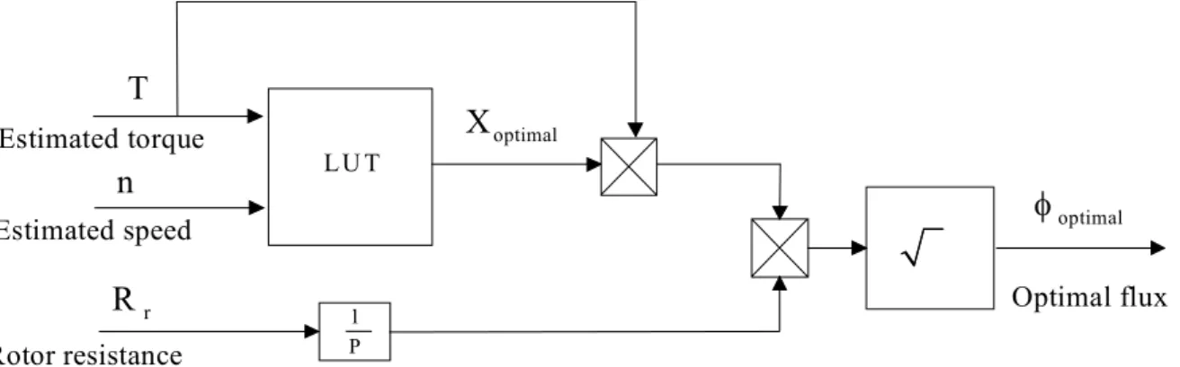
2) While running the motor, the torque is estimated by an observer and from the look up table the optimal flux is read (on-line). A PC was used for the on-line control. Figure 2.5 shows the block diagram of the optimal air gap flux calculation from the estimated torque.
The proposed loss model can be used in drives with scalar control as well as in drives with vector control.
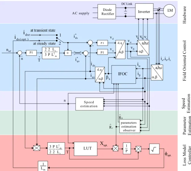
In vector control the rotor speed is measured using a speed sensor or calculated based on the electrical motor quantities (speed-sensorless). The interest in speed sensorless control emerged from practical application where high control quality is required but the speed sensor is either difficult to use due to technical reasons, or too expensive. So, using the proposed loss model to improve the efficiency of speed sensorless indirect field oriented controlled induction motor is suggested in this the-sis. The block diagram is as shown in Figure 2.6.
3 0 0 6 0 0 9 0 0 1 2 0 0 1 5 0 0 0 0 .5 1 0 .5 0 .6 0 .7 0 .8 0 .9 1 S p ee d (rp m ) Lo ad T o rq ue (p .u) Opti mal F lux ( p.u)
Figure 2.4: The optimal air gap flux for different load torques and different speeds. LU T optimal X r R T 1 P optimal φ n Estimated torque Estimated speed Rotor resistance Optimal flux
2.5 Implementation of the proposed loss model 19
The block diagram consists of four blocks. FOC, speed estimation, parameters es-timation observer, and proposed loss model block diagrams. The following sections explain each block separately.
2.5.1. FOC block diagram
In general, the field-oriented control can control the rotor flux linkage and the torque independently.
Values of the flux producing current component i*ds and the torque producing
cur-rent component *
q s
i are given. Each of these two components is controlled by a PI
controller. The controller output is the voltage vector in dq-reference frame, which transformed into αβ-reference frame by a vector rotator. Then, the switching times are calculated and the inverter impresses the voltage vector on the motor. Another vector rotator transforms the measured currents into the dq- reference frame. The re-sulting components are sent to the current controllers.
The angular position of the rotor flux linkage βk, which is required by the vector
ro-tators, is calculated by indirect means (IFOC) [33], from the measured currents and the estimated rotor speed.
The field-oriented control is primarily a current control. It is used together with a higher-level speed control. The speed controller calculates the torque producing cur-rent component as a function of the speed, which evaluated by the curcur-rent controller. So, the controller is a cascade control structure. That means that the outer control
AC supply , α β iα iβ a,b,c d, q , α β vα vβ b v vc ref n − Inverter r 2 m L 2 2 3 P L m 1 L I.M Diode Rectifier , αβ a v ds i * ds i − P I P I − IFOC d, q , α β βk a b c i ,i ,i a,b,c S p eed estim ation parameters estimation observer r R∧ d v q v opt. φ 1 P opt. X L U T P I n qs i T∗ ÷ dsr i 2 m r L 3 P 2 2 L S R∧ ds ( opt.) i T n Ha rd wa re Fi el d O riented C ont ro l Par ame te r Es ti m at io n Speed Es ti m at io n L os s Mode l C ont ro ll er * qs i DC Link 1 2
Figure 2.6: The optimal flux loss model based on speed sensorless vector control induction motor block diagram.
loop is speed controller controls the speed, its output is the reference torque. The in-ner controller is the current control loop, which controls the current to its reference values that is calculated from the reference torque value.
2.5.1.1. PI current controller
The current control loop of d-axis is working as follows. In the transient, such as at the beginning of the operation (motor starting) and in case of load changing, the
ref-erence flux-forming current component *
d s
i is established to the rated value idsr (=2.9A). In steady-state, the reference current i*d s is reduced to the optimal value
ds(opt.)
i
that is generated from the loss model controller. The loss model controllerbe-comes effective only at steady-state condition. That is, when the speed error ap-proaches zero.
The simplified current control loop of q-axis is as shown in Figure 2.7, where the coupling inductances between the d-q axes are neglected. The control’s time delay (included inverter reaction time) is represented by a first order lag element with a time constant TD = 1.5Ts where Ts is the sampling time [34]. The converter gain kc is
the relation between the numerical evaluation in the computer (digital controller) and the real output voltage. In this case the resolution scale used was 4000 (12 bits) for the complete line to line voltage (2/3 DC-Link voltage), which is calculated as follows
dc
c 2/3U
k =
4000 ,
for Udc=600 V, so kc=0.1.
The electrical gain kelecand the electrical time constant Telec of the motor are respec-tively
elec s k =1/ R
elec s s T =l / R
The PI controller setting according to the amplitude optimum criteria and its trans-fer function is represented as follows [34]
( ) i R p i 1+sT G s =K sT
The coefficients kp and Ti are calculated as follows s p c D l K = 2k T i elec T =T i p i 1+T s K T s c D k T s+1 * q U (s) elec elec k T s+1 q U (s) e(s) q I (s) E(s) Plant D elay C o n tro l tim e d elay
P I C o n tro ller
* q I (s)
2.5 Implementation of the proposed loss model 21 2.5.2. Speed estimation
Field oriented control method is widely used for the induction motor drives. For high precision and high dynamic, a speed sensor is necessary for speed signal feed back. However, a speed encoder cannot be mounted in some cases. Such as motor drives in a hostile environment, high speed motor drives. Also, a speed encoder is undesirable in a drive because it adds cost, reliability problems, and the need for a shaft extension and mounting arrangement.
These entire problems are solved by using the sensorless vector control methods. Sensorless vector control of the induction motor is presented in [35-40].
The speed is estimated by measuring the motor terminal voltages and currents. The speed can be estimated by one of the following methods:
- slip calculation.
- direct synthesis from state equation (motor back EMF equations). - model referencing adaptive system.
- speed adaptive flux observer. - extend kalman filter.
- slot harmonics.
- injection of auxiliary signal on salient rotor.
The aim is to improve the efficiency of the sensorless controlled induction motor by the suggested loss model, and not to investigate a new method or develop one of the known speed estimation methods. So, here the speed is estimated from mo-tor back EMF equations [56], which is easy to implement but its disadvantage that it does not work at standstill.
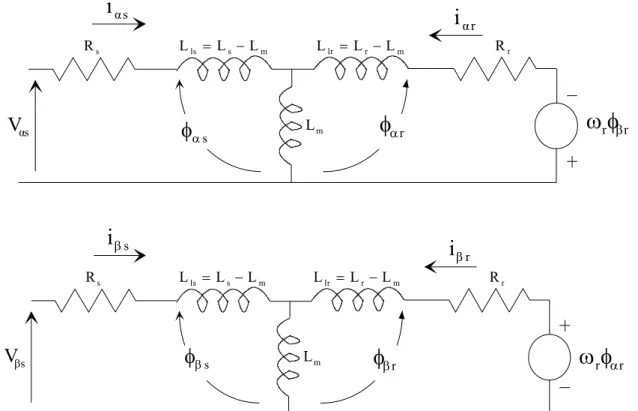
From the equivalent circuit of the induction motor in the stationary reference frame (α β, ) [16], as shown in Figure 2.8, rotor voltage equations are as follows
r R lr r m L = L −L ls s m L = L −L s R m L αs
i
αri
αsV
φ
αr s αφ
ω φ
r βr r αrω φ
r R lr r m L =L −L ls s m L = L −L s R m L si
β ri
β s Vβφ
βsφ
βrr r r r r r r r r r R i 0 R i 0 α α β β β α + ρ φ + ω φ = + ρ φ − ω φ = 2.33 where ρ= d/dt
The rotor currents are
αr αr m αs r βr βr m βs r 1 i = ( -L i ) L 1 i = ( -L i ) L φ φ 2.34
Resolving equation (2.33) and using (2.34), the estimated speeds are
r r m r r r s r r r r R R L ( i ) / A / L L β β β α α ω = ρφ + φ − φ = φ 2.35 r r m r r r s r r r r R R L ( i ) / B / L L α α α β β ω = −ρφ − φ + φ = φ 2.36
While the rotor flux components are calculated from the stator flux and stator cur-rent components as follows
r r s s s m r r s s s m L ( L i ) L L ( L i ) L α α α β β β φ = φ − σ φ = φ − σ
and σ =(L Ls r −L ) / L L2m r s (Blondel’s leakage factor)
The stator flux components are estimated by integrating the stator back- EMF us-ing a low pass filter.
s s s s s s s s 1 (V R i ) s a 1 (V R i ) s a α α α β β β φ = − + φ = − +
Where (a) is the cut-off frequency (a=3 Hz), (s) is Laplace Operator.
The numerator of equation (2.35) depends on the current component
i
βs, and thenumerator of equation (2.36) depends on the current component
i
αs , but theaccu-rate calculation of each component differs from the other due to a difference of the accuracy in measuring the three motor currents. So, it is better and more accurate to include the two current components
i
αsandi
βs in one equation as followsEquation (2.35) can be rewritten as
2 2 r r r 2 2 r r r r
A
A
α β α α α βφ +φ
ω =
=
φ
φ
φ +φ
or 2 2 2 2 αr βr 2 2 αr αr r 2 2 αr βrA
A
+
ω
=
+
φ
φ
φ
φ
φ
φ
2.372.5 Implementation of the proposed loss model 23 r r A B α β = φ φ 2.38 By inserting equation (2.38) in (2.37) the estimated speed is
2 2 2 2 r r 2 2 r r r 2 2 r r A B α β α β α β φ + φ φ φ ω = φ +φ 2 2 r 2 2 r r A B α β + ω = φ + φ
The block diagram of speed estimation is as shown in Figure 2.9.
The indirect field oriented control of an induction motor is sensitive to motor pa-rameters variation. Especially, rotor and stator resistances vary with the motor tem-perature.
Additionally, the proposed loss model controller depends on the motor parameters. Therefore, an on-line estimation of the motor parameters is necessary for the IFOC and for the proposed loss model. The following section explains the estimation of the stator and rotor resistances by using the parameter adaptive observer [28].
2.5.3. Parameters estimation
A standard smooth air gap model for the induction motor can be described by a state equation in stator reference frame as following.
d
x Ax Bu
dt = + 2.39
y Cx= 2.40
where
u= v
⎡
⎣
αsv
βs⎤
⎦
T : stator voltage vectorT αs βs αr βr
x= i
⎡
⎣
i
φ φ
⎤
⎦
: motor states αsV
s R αsI
∫ φαs mr L L r r R -L d -dt r m r R L L βsV
s R βsI
∫ βs φ mr L L φβr r r R L d dt −R LLr mr X X X X ÷ω
r αrφ
Ba
a
A s L σ s L σT
αs βs
y= i⎡⎣ i ⎤⎦ : stator current components
11 12 21 22 A A A A A ⎡ ⎤ = ⎢ ⎥ ⎣ ⎦ ,
[
]
T 1 2 B= B B , C=[
C C1 2]
T and A11= −{
R /( L ) (1s σ s + − σ στ) /( r) I a I}
= r11 A12 =L /( L L ) 1/( )Im σ s r{
τ − ωr rJ}
=a I a Jr12 + i12 A21 =(L / )I a Im τr = r 21 A22 = −(1/ )Iτ + ω =r rJ a I a Jr 22 + i22 B1=1/( L )I b Iσ s = 1 ,σ = −(1 L / L L )2m r s 1 0 I 0 1 ⎡ ⎤ = ⎢ ⎥ ⎣ ⎦ J 0 1 1 0 − ⎡ ⎤ = ⎢− ⎥ ⎣ ⎦ C1=I B2 C2 0 0 0 0 ⎡ ⎤ = = ⎢ ⎥ ⎣ ⎦Figure 2.10 shows Luenberger observer which estimates the stator current and the rotor flux in stator reference frame by the following equations.
L L L dx Ax Bu G(y y) A x B u dt = + + − = + 2.41
y Cx
=
2.42 where L A = +A GC ,BL =[
B −G]
, uL =[
u y]
T s s r rx=⎣⎡iα iβ φα φβ ⎦⎤ : the estimated states of the motor
T s s u= ⎣⎡vα vβ ⎤⎦ y = ⎣⎡iαs iβs⎤⎦T T s s y= ⎣⎡iα iβ ⎤⎦ T s s r r x=⎣⎡iα iβ φα φβ ⎤⎦ d x d t B C G A
∫
T s s y= ⎣⎡iα iβ ⎤⎦ Induction M otor s rR ,
τ
Adaptive schem e2.5 Implementation of the proposed loss model 25
T s s y= ⎣⎡iα iβ ⎤⎦
: the estimated output of the observer
T 1 2 3 4 2 1 4 3 g g g g G g g g g ⎡ ⎤ = ⎢− − ⎥
⎣ ⎦ : the observer gain matrix
Coefficients of the observer gain matrix G are chosen so that the Luenberger ob-server can be stable.
The most frequently used method is based on the fact that the observer eigenval-ues are chosen in such a way that they are proportional to the motor eigenvaleigenval-ues [41]. The induction motor itself is stable, so the observer is also stable in usual opera-tion. Coefficients of G matrix are
1 r11 r22
g
= −
(k 1)(a
+
a )
g
2=
(k 1)a
−
i22
g
3=
(k
2−
1)(ca
r11+
a ) c(k 1)(a
r 21−
−
r11+
a )
r 22
g
4= −
c(k 1)a
−
i22, c ( L L ) / L
= σ
s r mFigure 2.11 shows the eigenvalues for different values for (k) by solving the follow-ing equation.
L
A − λ =I 0 , (λ) is eigenvalues
For k = 0, 0.2, 0.6,1, and 1.1 all roots are negative and the observer is stable, but for k=1.2 and 1.5 the roots are positive and negative (observer is not stable).
In Figure 2.10 the induction motor (equation 2.39 and 2.40) represents the refer-ence model, while Luenberger observer (equation 2.41 and 2.42) is considered as adjustable model where it includes unknown parameters. From the error between the reference model and adjustable model, the stator resistance and the rotor time con-stant are calculated from the following adaptive scheme.
The difference between the estimated output and the real (measured) one is