Estimating the local average treatment effect
of R&D subsidies in a pan-European program
Paul Hünermund and Dirk Czarnitzki
Estimating the Local Average Treatment
Effect of R&D Subsidies in a
Pan-European Program
Paul H¨
unermund
∗Dirk Czarnitzki
†April 2016
We investigate the effect of Europe’s largest multilateral subsidy program for R&D-performing, small and medium-sized enterprises on firm growth. The program was organized under a specific budget allocation rule, referred to as Virtual Common Pot (VCP), which is designed to avoid cross-subsidization between participating countries. This rule creates exogenous variation in treatment status and allows us to identify the local average treatment effect of public R&D grants. In addition, we compare the program’s effect under the VCP rule with the standard situation of a Real Common Pot (RCP), where program authorities allocate a single budget according to uniform project evaluation criteria. Our estimates suggest no average effect of grants on firm growth but treatment effects are heterogeneous and increase with project quality. A Real Common Pot would have reduced the cost of policy-induced job creation by 27%. We discuss the implications of our findings for the coordination of national policy programs within the European Research Area.
Key words: Joint Programming Iniatives, R&D Policy, Virtual Common Pot, Instrumental Variable Estimation, European Research Area
JEL classification: O38, H25, C31
∗
KU Leuven, Department of Managerial Economics, Strategy and Innovation, Belgium, and Centre for European Economic Research (ZEW), Mannheim/Germany, Department of Industrial Economics and International Management. E-mail: [email protected]
†
KU Leuven, Department of Managerial Economics, Strategy and Innovation, Belgium, Center for R&D Monitoring (ECOOM) at KU Leuven, and Centre for European Economic Research.
1. INTRODUCTION
All OECD countries have policies in place that aim to support private research and development (R&D) activities. The rationale for these public interventions lies in preva-lent forms of market failure associated with the financing of R&D projects (Hall and Lerner, 2010). Limited possibilities to appropriate the returns of R&D investments (Ar-row, 1962; Aghion and Howitt, 1997) and positive externalities of knowledge production (Griliches, 1997; Bloom et al., 2013) result in a socially optimal level of R&D that ex-ceeds the aggregate investment level provided by markets. A pervasive problem for the design of subsidy programs, however, is to target R&D projects that are beneficial to society but at the same time not privately profitable. Otherwise grants will be ineffective in stimulating additional R&D (”additionality”) and instead displace (”crowd-out”) pri-vate investment (Wallsten, 2000). Because the screening of financially-constrained firms with good ideas is a difficult task (Hottenrott and Peters, 2012), critical voices question whether public policy programs are useful at all to correct market failures (Lerner, 2013). Researchers who want to investigate empirically the effect of R&D grants on firm performance face a well-understood endogeneity problem (David et al., 2000). Grants are rarely allocated randomly. Firms with high returns to R&D activities self-select into applying for a subsidy based on an individual cost-benefit analysis. Moreover, public authorities usually choose the most promising projects from a pool of applicants (”cream-skimming”). These two mechanisms induce a positive selection of firms with higher growth potential to participate in an R&D subsidy program.
Instrumental variable techniques, which exploit quasi-random variation in treatment status in order to address the problem of selection, are limited because it is diffi-cult to find suitable instruments in the context of R&D subsidies (Hussinger, 2008). Other popular econometric methods are nonparametric matching estimators (Almus and Czarnitzki, 2003; Czarnitzki and Lopes-Bento, 2013), difference-in-differences
esti-mators (Lach, 2002), regression discontinuity designs (Bronzini and Iachini, 2014), and estimation based on structural models (Takalo et al., 2013). Partly because of this va-riety of methodological approaches the findings on the effectiveness of R&D subsidies in the literature are mixed.
The aims of this study are twofold: (1) to evaluate the effect of a large pan-European subsidy program, which promoted international research collaborations of small and medium-sized enterprises, and (2) to propose a new instrument based on a specific budget allocation rule within the program to overcome the aforementioned selection bias.
1.1. The Eurostars Joint Programming Initiative
Article 185 of theTreaty on the Functioning of the European Unionenables the European Commission to coordinate and financially support subsidy programs for pre-commercial R&D that are jointly undertaken by several member states. These Joint Programming Initiatives1 (JPI) constitute the broader policy tool to achieve an integration of national innovation systems towards aEuropean Research Area (ERA). They are also an integral part of the Innovation Union Flagship Initiative—Europe’s 10-year strategy to foster innovation-led growth, competitiveness, and scientific excellence.2
TheEurostars Joint Programme(Eurostars hereafter) was launched in 2008 to support R&D-performing small and medium-sized enterprises (SME).3 Until 2013, the program allocated a total estimated budget of EUR 472 million in ten application rounds (called “cutoffs”). The 33 participating countries contributed a total of EUR 372 million finan-cial resources. EUR 100 million came from the 7th Framework Programme for Research
1
http://ec.europa.eu/research/era/joint-programming-initiatives_en.html 2
http://ec.europa.eu/jrc/en/research-topic/research-and-innovation-policies
3According to the standard definition employed by the EU an SME has less than 250 employees. In
addition, 10% of the work force (in full time equivalents) must be occupied with R&D activities or 10% of annual turnover must be dedicated to R&D in order to qualify as R&D-performing (these requirements have been lowered in later cutoffs). In a few exceptional cases, firms in our data seem to have been larger than this threshold. This is likely due to deviating rules at the national level.
and Technological Development on behalf of the European Commission. Eurostars was coordinated by EUREKA, a research network of European countries4 that aims at sup-porting pre-commercial but close-to-market R&D for civilian purposes. Its secretariat is based in Brussels.
Projects in Eurostars needed to be conducted by an international consortium of at least two SME from different countries. Larger companies and science-based partners, such as universities and research institutes, were also allowed to take part in the project. In each cutoff, project proposals were subject to a central evaluation process. Applicants had to provide detailed information about the envisaged R&D activities, work pack-ages, and expected costs. Based on this information, ESE carried out a basic eligibility check regarding administrative requirements. Subsequently, an application underwent an in-depth analysis by at least two independent technical experts. These experts rated projects according to three equally important quality criteria
1. Basic assessment: the consortium itself, its participants’ capabilities, the project plan, and financial aspects
2. Technology and innovation: the R&D activities to be conducted in the project, the degree of innovation, and the technological profile
3. Market and competitiveness: the market opportunities (size, geography, potential, time and risk), return on investment, and strategic importance of the project
(see Eurostar’s Final Evaluation Report, p. 185). Based on the experts’ reports, projects were given an overall evaluation score, ranging from 0 to 600 (600 being the best score), and the proposals were ranked accordingly. Eurostars applied a general quality threshold of 402 below which proposals were not considered eligible for funding.
4
The EU28 and five associated countries: Iceland, Israel, Norway, Switzerland, and Turkey.
Participating countries in Eurostars were committed to allocate their earmarked bud-gets strictly according to the central evaluation ranking. However, there was no common program budget but rather R&D grants were allocated individually by every participat-ing country only to their respective national applicants. Under this allocation rule, referred to as Virtual Common Pot (VCP), a project could only receive funding if fi-nancial resources were sufficiently available in all countries involved in the consortium. If only one country ran out of budget the entire project was rejected. These additional national budget constraints created variation in the funding of projects with nearly equal evaluation scores. For some projects budget constraints were binding whereas for other consortia, because the partners came from different countries, budget constraints were still slack. This stands in contrast to a Real Common Pot (RCP), under which all projects would be funded until a common budget is exhausted.
The following example illustrates the working of a VCP: Let there be four countries, A, B, C, and D, participating in the program. In each country there is sufficient budget to fund two R&D grants to national participants. Table 1 lists the outcome of a fictitious quality ranking of six project proposals by different international consortia. Under a VCP the first-ranked project can be funded, but subsequently country B’s budget is exhausted. Consequently, the second-ranked project receives no funding. For the third-ranked there are again sufficient national budgets available and the project can be granted. Under an RCP, all projects up to rank three would receive funding until the common program budget of eight available grants is exhausted. However, no participant from country D would receive a grant under such an allocation rule. This hypothetical example demonstrates how a VCP creates variation in funding at different evaluation ranks and that funded projects have a lower average quality under a VCP compared to an RCP. Figure A.2 gives an impression about the actual variation that occurred in the ten cutoffs of Eurostars.
Table 1: The allocation of a Virtual Common Pot (hypothetical example)
Quality Rank Consortium VCP RCP
1 A, B, B X X 2 B, B, C X 3 A, C X X 4 A, B, C, D 5 C, D, D X 6 A, C, D
instrument in a nonparametric instrumental variable estimation. Because financial con-tributions to Eurostars by participating countries were not disclosed to applicants, it is unlikely that firms were able to manipulate their funding status by means of strategic partner choice, which would undermine the credibility of the proposed instrument. We provide further survey evidence to substantiate this claim. Our estimation results sug-gest that R&D grants had on average no significant effect on firm growth. In subsequent analyses, we investigate treatment effect heterogeneity depending on project evaluation scores and find positive effects for projects with higher quality. By investigating detailed application records for a subsample of our data we are able to reject the hypothesis that the absence of positive treatment effects is explained by crowding-out. Instead, the program partly funded low-quality projects that were ineffective in inducing firm growth. Our results have implications for the design of joint policy initiatives under the current European legal framework. We show that increasing treatment effects caused a relative inefficiency of a VCP compared to an RCP because projects with lower quality were funded where grants were less effective. According to our estimates, a job created by the program under an RCP would have cost 27% less than under the VCP.
The remainder of the paper is organized as follows. Section 2 describes our empirical methodology and presents the data. Section 3 shows results of the estimation and the counterfactual analysis. Section 4 discusses the implications of our findings and concludes.
2. DATA AND SETUP
2.1. Nonparametric Instrumental Variable Estimation
In the presentation of the empirical model we follow the notation in Fr¨olich and Lechner (2014). Let Y be an outcome variable,D be a binary treatment variable, and Z be an instrumental variable. Consider the general non-additive model (see Figure A.1 for a graphical representation)
Y =ϕ(D, UY, UY D, UY Z, UY DZ)
D=ξ(Z, UD, UY D, UDZ, UY DZ) (1)
Z=ζ(UZ, UY Z, UDZ, UY DZ)
with ϕ, ξ, ζ being unknown functions and the U-variables being mutually independent random variables. This notation makes explicit that there are some influence factors that only affect one variable, UY, UD, UZ, some affect two at a time, UY D, UDZ, UY Z,
and some factors have an influence on all variables, UY DZ. In the tradition of the
potential outcome framework (Rubin, 1974, 1978), we define
Yid=ϕ(d, Ui,Y, Ui,Y D, Ui,Y Z, Ui,Y DZ), d= 0,1
as firm i’s potential outcome. Yi1 denotes the outcome under treatment (D= 1) andYi0 in the counterfactual state (D= 0). For ease of notation we will omit the firm subscript in what follows when it causes no confusion.
The notion ofZ being an instrumental variable follows from the exclusion restriction thatZ is not an argument of the functionϕ. Consider the case of a binary instrument, Z ∈ {0,1}. Then, there are four possible types of firms,T, in the population depending
on the state of Z.
Compliers (T =c) : DZ=0 = 0 and DZ=1= 1, Defiers (T =d) : DZ=0 = 1 and DZ=1= 0, Always-treated (T =a) : DZ=0 = 1 and DZ=1= 1, Never-treated (T =n) : DZ=0 = 0 and DZ=1= 0.
The typeT categorizes how the treatment status of a firm changes when the instrument changes. Compliers are those firms that have a treatment status of one if the instrument is equal to one and zero otherwise.
The standard literature on instrumental variable estimation assumes UY Z, UDZ, and
UY DZ to be empty, i.e.,Z is independent of potential outcomes and types
(Yd, T)⊥⊥Z.
Under the additional assumption of ξ being monotonically increasing in Z, such that there are no defiers6, Imbens and Angrist (1994) show that the local average treatment
effect (LATE) for the subpopulation of compliers is identified as
E[Y1−Y0|T =c] = E[Y|Z = 1]−E[Y|Z = 0]
E[D|Z = 1]−E[D|Z = 0]. (2) In the case of Eurostars, we exploit the fact that for some firms in a project consortium the respective national budget was exhausted as an instrument. In this case all firms within the project consortium were denied funding. To follow the usual notation that treatment is monotone increasing in the instrument, we define Z = 0 as the case when
6
Alternatively, ξ could be monotonically decreasing in Z such that there only exist defiers but no compliers.
at least one respective national budget was exhausted and Z = 1 when all respective national budget constraints were still slack.
In our setting, we have perfect compliance to our instrument. No project was funded when budget constraints were binding and all applicants took up funding if they were still sufficiently available. Thus, D = Z and we can delete the second equation in (1) together with the variablesUY D, UDZ and UY DZ from the model. The denominator in
equation (2), the definition of the LATE, becomes equal to one.
We acknowledge the possibility that there might be factors UY Z that appear both in
ϕandζ and therefore influence outcomes and the instrument alike. We assume that we observe all these confounding factors and call themX from here on to comply with the standard notation in the literature. Conditional onX Z is a valid instrument
Yd⊥⊥Z |X.
However, the conditioning (also denoted as ”balancing”) is only feasible when the distribution of X has the same support for both values of the instrument. This as-sumption makes sure that the treatment propensity lies strictly between zero and one: 0<Pr(Z = 1|X)<1 (Heckman et al., 1998). Accordingly, we restrict our analysis to a region of common support defined as
S = Supp(X|Z = 1)∩Supp(X|Z = 0)
to be able to make reasonable comparisons between treated and non-treated firms. In-tegrating the difference in mean outcomes over X in the region of common support identifies the average treatment effect (ATE) for this region
This quantity can be estimated by nearest-neighbor or propensity score matching. Be-cause of perfect compliance the estimation procedure in the instrumental variable setup is equivalent to a ”selection on observables”-approach (Cameron and Trivedi, 2005). However, our instrument is not able to shift treatment in all regions of Supp(X). Most notably, we can estimate the treatment effect of Eurostars funding only for specific re-gions of the project evaluation score, where there is sufficient variation in the funding status (see Figure A.2). Because of this local definition of the treatment effect condi-tional onX∈S, for a well-defined subpopulation, we present our estimation strategy in the general framework of the LATE (Imbens, 2010).
We employ propensity score matching to alleviate the dimensionality problem (Heck-man et al., 1998; Abadie and Imbens, 2016) of conditioning on multiple covariates. Rosenbaum and Rubin (1983) establish that balancing is feasible conditional only on the one-dimensional propensity score Pr(Z = 1|X) =P(X)
Yd⊥⊥Z |P(X).
We estimateP(X) by Probit regression and match an observation with its nearest neigh-bor according to the estimated propensity score. Abadie and Imbens (2016) derive the large sample distribution of the propensity score matching estimator. Note that we as-sume that potential outcomes do not depend on the actual treatment exposure. Hence, the assumption of causal effect stability or stable unit treatment values (SUTVA) is fulfilled.
2.2. Data
We study the official Eurostars application records provided by the EUREKA secretariat (ESE). To assess the effect of R&D subsidies on firm performance, we combine our data set with employment data until 2013 from Bureau van Dijk’s Amadeus database. We
restrict the analysis to applications until cutoff round 7 (which took place in September 2011) to allow for sufficient time for positive effects of the program to materialize. We drop from the sample all non-SME such as universities, research institutes or larger com-panies. In addition, we drop applications from countries not associated with EUREKA7 and from Malta as there were few and Malta only joined the program in cutoff 6.
We construct a measure of employment growth (Employment Growth) between the year before application (t−1) and 2013 divided by the number of elapsed years
Empl2013−Emplt−1 2013−t−1
.
When data is missing for the respective years we adjust this time window but make sure that at least two years have passed before we compare the difference in employment levels8. Our choice of outcome variable is motivated by the fact that increasing levels of employment are a general indicator of firm growth and competitiveness. Moreover, job creation was an explicit goal of the program for public authorities (Final Evaluation Report, p. 10).
As a baseline set of covariates we condition on the technology class of a proposed project (Technology Class, see Table 2), the cutoff round (Cutoff) in which a project was applied for, and the number of employees one year before application (Employment Start). We further control for the cumulative patent stock (Patent Stock) of a firm at application date.9 Most relevant for identification is to include the project evaluation scores (Score) in the matching. Score directly affects the treatment propensity of a project as well as it has a likely effect on potential outcomes. By comparing direct
7
Applicants from non-EUREKA countries had the possibility to participate as self-funded consortium partners.
8
We also studied the effect on compound annual growth rates and found qualitatively similar results. For the following counterfactual analysis, however, we found absolute employment growth to be a more conservative measure for out-of-sample predictions.
9We count patent applications at the European Patent Office since 1985 in thePATSTAT database.
We also checked the effect of assuming an annual discount rate of 15% on the knowledge stock and found very similar results.
neighbors in the quality ranking of a certain cutoff we make sure that funded and non-funded projects are of similar quality.
The probability to receive funding in Eurostars was close to one for proposals that received high project evaluation scores because budgets for them were still slack. This violates the common support assumption introduced in Section 2.1. The same applies for project proposals that did not pass the quality threshold as their treatment propensity was zero by design. We thus restrict our analysis to projects above that received aScore
between 400 and 510. In this range there was sufficient variation in funding status (see Figure A.2).
Our final data set contains 767 observations. Table 2 shows descriptives statistics of the variables in our sample. With an average number of 28 employees firms were relatively small when they applied to Eurostars. On average they hired 1.3 new employees per year which indicates a dynamic growth of these firms. However,Employment Growthshows a high variance in the sample. This is most likely the result of the diverging macroeconomic environment within Europe during the years 2008 to 2013. Nearly two thirds (64%) of the firms in the sample received funding by Eurostars.10 Projects predominantly came from the fields of information and communications technology (ICT) and engineering.
Unlike many other studies on R&D subsidies, our data allow us to compare treated and non-treated firms that both applied for funding by Eurostars. Often there is only information about the identity of treated firms available and a control group needs to be drawn randomly from the population of all firms. However, firms select into applying for R&D subsidies based on the prospective gains of receiving a subsidy and thus based on potential outcomes (Takalo et al., 2013). Many firms refrain from ever applying to a program, especially when there are non-negligible application costs involved due to administrative requirements and the need to coordinate a joint proposal. The subpop-ulation of subsidy applicants might therefore possess substantially different unobserved
characteristics (Blanes and Busom, 2004). Our study avoids this potential source of confounding. We define the relevant population of interest as all potential applicants to a EuropeanJoint Programming Initiative targeted at R&D-performing SME.
2.3. Instrument Validity
We argue that conditional on the evaluation rank of a firm (or equivalently, on both
Score and Cutoff) the availability of national budget resources is independent of poten-tial outcomes. The Virtual Common Pot introduces variation in the funding status for proposals that were evaluated to be of the same overall quality by independent technical experts (see Figure A.2). The region of variation is larger than in, for example, stud-ies that employ a Regression Discontinuity Design (Hahn et al., 2001), where there is only one threshold around which variation in treatment status can be exploited. Con-sequently, treatment effects can be identified for a larger share of the population. In addition, treatment status perfectly complies to our instrument which means there are no always-takers and never-takers in the region of common support.
Although countries were able to adjust their budget contributions even after observing the evaluation ranking, they were committed to the allocation rule under the VCP. Thus, there was no room for discretionary treatment of selected firms by national agencies. However, since national budgets11vary in their size (relative to demand) the treatment propensity differs for firms from different countries even after controlling for Scores. Therefore, the treatment propensity could potentially be correlated with macroeconomic effects at the country level which affect potential outcomes. To avoid such a confounding effect, we condition on a set of country groups in the estimation of the propensity score 11The size of national budgets and therefore the commitment to a multilateral R&D subsidy program
such as Eurostars, also in relation to existing national programs, depends on various political rea-sons. It appears that not all countries were successful in forecasting the actual demand for funding. Especially large countries—which were attractive collaboration partners because of, e.g., market access—were likely to contribute too small budgets compared to the number of applications. There is no clear correlation in the data between relative budget size, on the one hand, and the size of the country or its exposure to credit market risks in the European sovereign debt crisis, on the other hand (see also the Final Evaluation Report, Figure 6-10).
Table 2: Summary statistics
Mean Std. Dev. Min. Max.
Employment Growth 1.294 6.295 -57 77.667 Employment Start 28.072 44.037 1 375 Funding 0.644 0 1 Score 444.581 29.358 400 510 Patent Stock 10.952 28.844 0 141 Growth Rate -0.219 1.143 -5.213 2.7 Self-funding 0.09 0 1 Technology Class: ICT 0.319 0 1 Engineering 0.327 0 1
Bioscience, Pharma & Chemistry 0.219 0 1
Other 0.134 0 1 Cutoff Dummies: Cutoff 1 0.168 0 1 Cutoff 2 0.141 0 1 Cutoff 3 0.155 0 1 Cutoff 4 0.125 0 1 Cutoff 5 0.128 0 1 Cutoff 6 0.158 0 1 Cutoff 7 0.125 0 1 Country Groups: DE 0.188 0 1 FR 0.081 0 1 IT 0.073 0 1 UK, IE 0.025 0 1 NL, BE, LU 0.117 0 1 AT, CH 0.066 0 1
FI, SE, NO, DK 0.169 0 1
GR, PT, ES 0.175 0 1
EU since 2004 0.106 0 1
N = 767. EU since 2004: member states that joined the EU in 2004 (Cyprus, Czech Republic, Estonia, Hungary, Latvia, Lithuania, Poland, Slovakia, and Slovenia), in 2007 (Romania), and in 2013 (Croatia).
(see Table 2).
The VCP also introduces variation in treatment within countries. Some firms did not receive funding because national budget of some partners in their consortium were exhausted. By contrast, for other firms from the same country all budgets were still slack. This mitigates the problem of cross-country comparisons. Nevertheless, the number of applications in some countries were too low such that we are forced to group countries together. Additionally, we control for the average Growth Rate of a country’s GDP during 2008 until 2013 to allow for heterogeneity within the groups and to capture confounding effects of different growth trajectories.
There is a potential concern about the strategic choice of collaboration partners in order to maximize the funding probability. Firms with high growth potential could have chosen their partners with regard to the relative size of their national budgets; and such a strategic behavior could possibly bias our estimates. In the course of the official evaluation of Eurostars on behalf of EUREKA and the European Commission, the expert group in charge conducted an online survey about firms’ experience with the program. One item in the survey12 was concerned with the question of strategic partner choice. Respondents were asked to state their level of agreement to the following statement on a five-point Likert scale:
“We chose our project partners strategically from certain countries because we believe that differences in national budgets affect the probability to obtain funding by Eurostars.”
15.9% of the responding firms in our sample agreed with the statement that they chose their project partners specifically from certain countries. 4.6% indicated a strong agreement with the statement. Around 79% of firms had a neutral opinion, disagreed or 12Details about the survey can be found in the final report of the expert group (Final Evaluation Report,
2014). Important for our purposes is that there was a reasonably high response rate by applicants and especially by both, funded and non-funded firms.
disagreed strongly. Other reasons of partner choice, such as technology transfer, access to new markets, or previously existing business relationships were much more important to respondents (Final Evaluation Report, Figure 6-5). In addition, even if firms were aware of the specific allocation rules within a VCP, information about national budgets was not public. Because there was no clear pattern between relative budget size and indicators such as country size or geography, it is questionable whether firms were able to effectively manipulate their chance to obtain funding by strategic partner choice.
Firms from countries with exhausted budgets had the possibility to self-fund their part of the project. That way, the other consortium member could still obtain funding from their national authorities. In around 9% (see Table 2) of the cases one partner in a consortium exercised this option. The decision to self-fund might be based on private information about the quality of a project and could thus be a sign for a very profitable venture. To hedge against a bias in our estimation we control for whether a consortium member decided to finance the project without public support.
3. EMPIRICAL RESULTS
3.1. Results of the Propensity Score Matching
Table 3 reports results of the propensity score matching. We present three specifica-tions: (1) with the baseline set of covariates, (2) includes the Country Groups, and (3) additionally incorporates the average Growth Rate of GDP and Self-Funding by firms in a consortium.
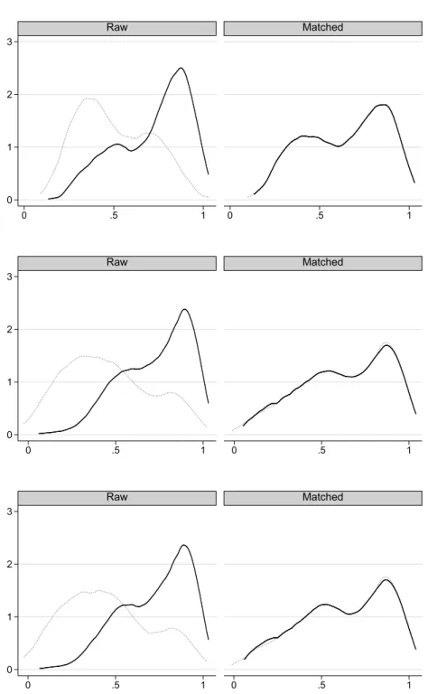
We apply a trimming method suggested by Crump et al. (2009) to guard against limited overlap. We only consider observations with an estimated propensity score in the interval [0.02,0.98] for the nearest-neighbor matching. Because the treatment propensity converges to one for high evaluation ranks (see Figure A.2) we thereby lose up to 34 observations from our sample in specification (3). Figure A.3 shows that this conservative
Table 3: Propensity score matching results (1) (2) (3) E[Y1−Y0|X∈S] 0.607 0.323 0.900 (0.490) (0.744) (0.797) Score X X X Employment Start X X X Cutoff X X X Technology X X X Patent Stock X X X Country Groups X X Growth Rate X Self-funding X Observations 761 738 733
Standard errors in parentheses: ∗ p <0.10, ∗∗ p <0.05,
∗∗∗
p <0.01
Notes: Estimated average treatment effect of R&D grants in the region of common support for three different sets of covariates. We discard observations with an estimated propensity score outside the interval [0.02,0.98] as it was suggested by Crump et al. (2009) to guarantee sufficient overlap.
approach results in a good overlap of the distribution of covariates for both treatment levels and a good matching. Table A.1 reports the Probit propensity score estimation results.
In all three specifications we find no significant average treatment effect of R&D subsidies on employment growth. Point estimates vary slightly depending on the set of covariates used in the estimation of the propensity score. Standard errors are quite large which reflects the substantial variation in the outcome variable that was already visible in the descriptive statistics.
3.2. Counterfactual Situation Under a Real Common Pot
Because of the additional national budget constraints under a Virtual Common Pot (VCP) compared to a Real Common Pot (RCP), the average project evaluation score of
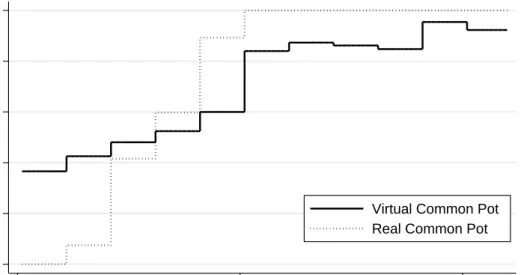
funded projects is lower under a VCP. We compute the counterfactual treatment status for firms in our sample if the same total budget allocated in Eurostars would have been allocated according to an RCP. Figure 1 depicts the treatment propensities depending on project evaluation scores. One can see that starting from a score of around 440, the probability to receive funding is higher under an RCP than under a VCP.
This creates a relative inefficiency of a VCP compared to an RCP when treatment effects are heterogeneous and increasing in evaluation scores. We analyze treatment effect heterogeneity for different scores by a two-step regression method. First, we perform a nearest-neighbor matching on the entire covariate vector, given in Table 3 specification (3), instead of the propensity score.13 Then, we compute the difference in employment growth between matched neighbors and regress these on scores to asses how treatment effects vary with project quality. Appendices A.3 and A.4 provide further detail on the method.
Figure 2 shows results for a local linear regression (LLR, Fan and Gijbels, 1996) and a fractional polynomial regression (FPR, Royston and Altman, 1994). The latter is an OLS regression on a higher-order polynomial, which additionally allows for logarithms and non-integer powers of the regressor. One can see that the insignificant average treatment effect conceals substantial heterogeneity depending on project qualities. Up to a score of around 430 point estimates are basically zero. For proposals with higher scores the treatment effects become larger, up to an average of around 2 employees hired per year. The 90% confidence interval starts excluding zero for scores between approximately 460 and 500. In the following we will interpret the results of the FPR because it is smoother than the LLR. Presumably this is an artifact of our limited sample size.
Given the estimated relationship between treatment effects and evaluation scores, a reallocation of the budget according to an RCP would increase the number of jobs created by the program because projects with higher average scores receive funding.
13
Table A.2 shows these matching results, which at the same time serve as a robustness check for our previous propensity score matching results.
Figure 1: Treatment propensity 0 .2 .4 .6 .8 1 400 450 500 Score
Virtual Common Pot Real Common Pot
Notes: Sample probabilities to receive funding at different project evaluation scores under a VCP compared to an RCP. Probabilities are calculated within 11 equidistant bins ofScores.
Table 4 shows results of a counterfactual analysis. In the factual situation under the VCP one job was created by an average grant size of EUR 97,899. Under an RCP the program would have been considerably more cost-effective, with just EUR 71,813 creating one job. This amounts to a reduction in costs of around 27%.
Because a switch to one common budget under an RCP might not be politically feasible, we investigate the effectiveness of a mixed funding allocation. The European Commission committed itself to contribute EUR 100 million to the Eurostars Joint Pro-gramming Initiative under the condition that participating countries provide a budget of at least EUR 300 million (Final Evaluation Report, p. 12) by themselves. The Commis-sion’s share was used to supplement the national budgets. We study the effectiveness of the program if 25% of Eurostars’ total budget would have been allocated according to an RCP. This counterfactual scenario conveys the notion that the EC could have allocated its budget strictly according to the evaluation ranking without taking national budget
Figure 2: Treatment effect heterogeneity -1 0 1 2 3 400 450 500 Score Local polynomial Fractional polynomial
Notes: Solid line: Fractional polynomial regression (Royston and Altman, 1994) of treatment effects on project scores with powers (2, 3, 3). Dotted line: local polynomial regression of treatment effects on project scores. Degree = 1, kernel = epanechnikov, bandwidth = 12.6. Figure A.4 shows confidence intervals for both regressions. For scores between 460 and 500 they do not include zero. Due to data limitations confidence regions become wide for higher scores.
Table 4: Counterfactual employment growth under a VCP vs. RCP
VCP RCP Mixed Mode
Number of funded firms 460 448 441
Average score of funded firms 451.0 459.4 454.3
Grant size divided by created jobs (EUR) 97,899 71,813 76,574
Notes: Counterfactual situation given treatment propensities (Figure 1) and average treat-ment effects (Figure 2) when total budget is allocated according to an RCP. Mixed mode allocation assumes 25% of the total budget in a cutoff round are allocated according to an RCP. The remaining national budgets are allocated according to the VCP funding rule. Employment growth is computed per firm from application year until 2013.
constraints into account. The remaining 75%, provided by the participating countries, would still have been allocated according to the VCP rule after the common budget was exhausted.
Table 4 shows that such a mixed mode works surprisingly well in our sample. A job created under this regime costs EUR 77,710 and is therefore around 22% cheaper than under a VCP. The major part of the impact on employment growth comes from projects with high evaluation scores (see Figure 2). A mixed mode makes sure that all these projects receive funding. On the contrary, this result demonstrates that a large part of the spent budget in Eurostars was ineffective in fostering employment growth. Although a mixed mode allocates grants to projects of lower average quality compared to an RCP, the resulting employment growth is at a comparable level as long as only the highest ranks are funded. For the remaining 75% of the budget it does not make much of a difference whether they are allocated according to a VCP or an RCP.
3.3. Financial Position of Eurostars Firms
Figure 2 reveals that Eurostars grants had no effect on firm growth for a large range of low-ranked projects. Usually the literature explains the absence of treatment effects with the presence of crowding-out. Firms that are perfectly able to finance their R&D projects by themselves still have an incentive to apply for grants because (less application
costs) they constitute a net transfer (Almus and Czarnitzki, 2003). However, it appears unlikely that firms with low-quality projects should be in a better financial situation to finance their R&D projects than their high-ranked counterparts (for which the treatment effect is positive).
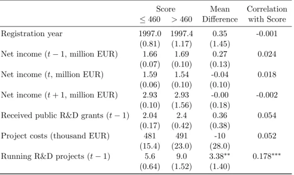
To test the hypothesis that financial constraints was especially prevalent among high-ranked firms we study information about the financial situation of firms available in the application records of Eurostars. Applicants had to disclose their net income according to their latest financial statement at application date. In addition, they were required to report past net income and expected income for the upcoming year. Firms also had to state their project costs since the subsidy amount was calculated on this basis. With cutoff round 5, the application form has been extended to cover the applicant’s age, the receipt of R&D grants prior to Eurostars, and the number of running R&D projects. We split the subsample of firms for which the respective variable is available at a score of 460, when the treatment effect of grants becomes distinguishable from zero, and compare groups means. In addition, we look at the correlation between variables and project evaluation scores.
Table 5 attests no differences related to the financial position of firms between the two groups. Also there is no statistically significant correlation between evaluation scores and net income. Firm age, which could facilitate capital market access, is on average the same across groups. The same holds for the size of the proposed R&D projects. Low-ranked firms thus did not apply with less costly projects that are easier to finance. Another argument speaking for the presence of crowding-out, specifically for firms with project of comparably low quality, is that these firms might find it easier to attract public money form other sources; e.g., because they are located in less developed regions on which there lies a distinct policy focus. With an average of around two grants received in the year before application, Eurostars applicants were generally quite successful in attracting public money, yet there is no significant difference between low and
high-Table 5: Evidence for financing constraints
Score Mean Correlation
≤460 >460 Difference with Score
Registration year 1997.0 1997.4 0.35 -0.001
(0.81) (1.17) (1.45)
Net income (t−1, million EUR) 1.66 1.69 0.27 0.024
(0.07) (0.10) (0.13)
Net income (t, million EUR) 1.59 1.54 -0.04 0.018
(0.06) (0.10) (0.10)
Net income (t+ 1, million EUR) 2.93 2.93 -0.00 -0.002
(0.10) (1.56) (0.18)
Received public R&D grants (t−1) 2.04 2.4 0.36 0.054
(0.17) (0.42) (0.38)
Project costs (thousand EUR) 481 491 -10 0.052
(15.4) (23.0) (28.0)
Running R&D projects (t−1) 5.6 9.0 3.38∗∗ 0.178∗∗∗
(0.64) (1.52) (1.40)
Standard errors in parentheses: ∗p <0.10,∗∗ p <0.05,∗∗∗p <0.01
Notes: The table provides additional information on the financing conditions of Eurostars firms depending on their position in the project quality ranking. Data for registration year, received public grants, and running R&D projects are only available for cutoff 5 to 7. The threshold of
Score= 460 marks where treatment effects of R&D grants become positive. Timet denotes the year of application. Financial data is according to latest financial statement at application date. Net income int+ 1 refers to one-year forecasts.
ranked firms. Only the number of running R&D projects are positively correlated with project evaluation scores. The fact that high-ranked firms were able to conduct are larger number of projects, however, provides even more evidence against their hypothesized financing constraints.
4. DISCUSSION
The independent variation in treatment status, which is induced by a Virtual Common Pot, allows us to identify the local average treatment effect of public R&D grants on firm growth. We find no significant average effect but substantial treatment effect het-erogeneity depending on project quality, i.e., the effectiveness of grants increases with the project evaluation score. A counterfactual analysis reveals that a VCP imposes
sub-stantial additional program costs compared to a Real Common Pot. A mixed budget allocation rule, by contrast, avoids parts of these extra costs.
Our study tackles several of the methodological problems researchers encounter when estimating the effectiveness of R&D subsidies. Frequently, public authorities only pub-lish data about funded projects. In this case, researchers usually rely on matched control samples from the population of all firms by imposing a selection-on-observables assump-tion. However, firms apply for R&D grants based on potential outcomes. Applicants potentially differ from non-applicants in unobserved characteristics. We avoid this prob-lem by restricting our analysis to firms that applied to Eurostars. Furthermore, we propose a new instrument, based on the specific VCP budget allocation rule, that deals with the problem of cream-skimming. Public authorities are held accountable to make good use of taxpayers’ money. They therefore rarely allocate subsidies randomly but rather try to choose the best projects from a list of applications. In a VCP cream-skimming is partly offset by the additional national budget constraints and thus grants are not solely allocated based on quality.
Our identification strategy relies on data about project evaluation scores. Knowledge about the authority’s quality ranking would also allow to identify local causal effects in a regression discontinuity design (see Howell, 2016, for a recent application). However, we are able to estimate effects for a larger share of the population than in an RDD, as we can exploit variation not only at one threshold but in a wider region of the evaluation ranking. The considerable treatment effect heterogeneity we find illustrates the desirability of an estimation approach that is less ”local”.
While the literature on R&D policies is concerned with the possibility that public grants are crowding out private investment–which diminishes their additionality–our results suggest that firms with a low treatment effect in our sample are neither in a better financial situation, nor do they have easier access to other sources of public support. Instead, Eurostars funded a non-negligible share of low-quality projects that
proved to be ineffective in pushing the firms’ growth trajectory. This is the case although projects were reviewed by independent technical experts and the program applied a general quality threshold. These results highlight that program authorities need to set minimum quality requirements carefully to avoid sponsoring fruitless R&D efforts. Nevertheless, public support for these types of projects could be justified by other policy goals different from firm growth, e.g., knowledge spillovers or international technology transfer.
A limitation of our study is that we only investigate the effect of R&D grants on one outcome variable.14 Other studies in the literature often consider their effect on investment in R&D (Z´u˜niga-Vincente et al., 2014). Unfortunately, information about R&D expenditures by firms is very scarce in databases covering the European economy as a whole, such as the Amadeus database used in this paper. We thus cannot contribute to a strain of literature that is concerned with the input additionality of R&D subsidy programs. Instead, we look at the output additionality of Eurostars in the policy-relevant dimension of firm growth and competitiveness.
The instrumental variable approach we pursue naturally gives rise to questions about the external validity of our results. We are only able to estimate local treatment effects in regions of the covariate support where our instrument has the power to influence the funding status. Indeed, we are completely agnostic about the size and sign of treatment effects in other regions of the evaluation ranking (i.e., below the quality threshold or above a score of 510). This is specifically related to a certain country composition in the region of common support.
As we argued earlier, the reasons why countries within Eurostars ran out of budget were not unidimensional and also not constant over time. There was no systematic pattern present, such as, that national budgets of small countries with a below average 14In unreported analyses we also studied the effect of Eurostars grants on the patent applications of
SME. We found neither statistically nor economically significant results; presumably, because research projects within Eurostars had a more applied and ”close-to-the-market” character.
GDP growth were exhausted the earliest. Instead, large countries often provided too few resources compared to the amount of applications they received. Also, actual demand for grants was difficult to forecast, as it varied over time. Consequently, our instrument is powerful enough to manipulate treatment status over a wide support of the geographical distribution in the sample. In any case, the region of common support, where the VCP introduces variation in treatment, is exactly the region of the evaluation ranking relevant for a comparison of a VCP versus an RCP.
Our results have important implications for innovation policy in Europe. In 2014, the successor program Eurostars 2 was launched under the European Horizon 2020 Framework Programme.15 Its earmarked budget increased significantly compared to Eurostars 1 with a contribution by the European Commission of EUR 287 million over six years. In addition, other Joint Programming Initiatives are also organized as a Virtual Common Pot.16
A VCP is designed to provide incentives for countries to contribute national budgets to a pan-European program and to avoid free-riding. Policy makers face important political constraints when they try to harmonize their innovation policies and promote cross-boarder research projects. In particular, countries are concerned that their taxpayers’ money could be used to subsidize research in other EU states. Moreover, there is a frequent debate in the European policy sphere about ”just return”—the question whether countries benefit from a policy program proportionally to what they pay into it. A VCP circumvents these concerns and is a tool to combine the goal of further policy harmonization with the EU’s highly federal structure.
However, our results illustrate that such a tool imposes non-negligible costs. Eurostars would have been much more cost-effective if it had been organized as a Real Common Pot. For a substantial share of the funded projects under a VCP grants had no additionality effect on firm growth. As a consequence, we also find no significantly positive average
15
http://ec.europa.eu/programmes/horizon2020/en/h2020-section/eurostars-programme 16Moretti and Villanova (2012) estimate that around 80% of joint calls are organized as a VCP.
effect of the program. We emphasize though that this conclusion should be taken with a grain of salt as we do not estimate treatment effects for the last three cutoff rounds within Eurostars 1 and we are not able to say anything about treatment effects for projects with very high evaluation scores outside of the common support.
A switch from a VCP to an RCP, although desirable from the point of view of efficiency, might not be politically feasible. We propose a mixed mode between a VCP and RCP to allocate joint research budgets. Under article 185 of theTreaty on the Functioning of the European Unionthe European Commission is allowed to contribute its own financial resources to Joint Programming Initiatives. In Eurostars the EC’s earmarked contribu-tion was 25%. If this budget had been allocated to the highest-ranked firms instead of supplementing the national budgets, a larger share of projects for which grants show a high degree of additionality would have been funded. Because the remaining share of the total budget could still have been allocated according to the VCP, discussions about “just return” could equally be avoided.
Although a mixed mode works extremely well in our sample and comes close to the first-best allocation under an RCP, this is a consequence of the shape of the estimated relationship between the treatment effect and project evaluation scores. The treatment effect is only positive for the highest-ranked projects. A mixed mode makes sure that all of these projects are funded. For the remaining projects with lower rankings it makes no significant difference whether they are funded under a VCP or an RCP. This does not need to be the case in general, e.g., when treatment effects are increasing linearly in project quality. Still, we think that a mixed mode, especially when the common RCP share comprises a significant part of the total budget, is more suitable than a pure Virtual Common Pot to trade-off between economic efficiency and political feasibility.
REFERENCES
Abadie, A. and Imbens, G. (2016). Matching on the Estimated Propensity Score. Econo-metrica, 84(2):781–807.
Abadie, A. and Imbens, G. W. (2006). Large Sample Properties of Matching Estimators for Average Treatment Effects. Econometrica, 74(1):235–267.
Abadie, A. and Imbens, G. W. (2011). Bias-Corrected Matching Estimators for Average Treatment Effects. Journal of Business & Economic Statistics, 29(1):1–11.
Aghion, P. and Howitt, P. (1997). Endogenous Growth Theory. The MIT Press, Cam-bridge.
Almus, M. and Czarnitzki, D. (2003). The effects of public R&D subsidies on firms’ innovation activities: the case of Eastern Germany. Journal of Business and Economic Statistics, 21:226–236.
Arrow, K. (1962). Economic welfare and the allocation of resources for invention. In Nelson, R., editor, The rate and direction of inventive activity: economic and social factors, pages 609–625. Princton University Press.
Balsmeier, B. and Pellens, M. (2015). How much does it cost to be a scientist? Journal of Technology Transfer.
Blanes, J. V. and Busom, I. (2004). Who participates in R&D subsidy programs? The case of Spanish manufacturing firms. Research Policy, 33:1459–1476.
Bloom, N., Schankerman, M., and Van Reenen, J. (2013). Identifying technology spillovers and product market rivalry. Econometrica, 81(4):1347–1393.
Bronzini, R. and Iachini, E. (2014). Are Incentives for R&D Effective. American Eco-nomic Journal: EcoEco-nomic Policy, 6(4):100–134.
Cameron, A. C. and Trivedi, P. K. (2005). Microeconometrics: Methods and Applica-tions. Cambridge University Press.
Crump, R. K., Hotz, V. J., Imbens, G. W., and Mitnik, O. A. (2009). Dealing with limited overlap in estimation of average treatment effects. Biometrika, 96(1):187–199. Czarnitzki, D. and Lopes-Bento, C. (2013). Value for money? New microeconometric
evidence on public R&D grants in Flanders. Research Policy, 42:76–89.
David, P. A., Hall, B. H., and Toole, A. A. (2000). Is public R&D a complement or substitute for private R&D? A review of the econometric evidence. Research Policy, 29:497–529.
Fan, J. and Gijbels, I. (1996). Local Polynomial Modelling and Its Applications. Chap-man & Hall, London.
Fr¨olich, M. and Lechner, M. (2014). Combining Matching and Nonparametric Instru-mental Variable Estimation: Theory and an Application to the Evaluation of Active Labour Market Policies. Journal of Applied Econometrics. forthcoming.
Griliches, Z. (1997). The search for R&D spillovers. The Scandinavian Journal of Economics, 94:29–47.
Hahn, J., Todd, P., and der Klaauw, W. V. (2001). Identification and Estimation of Treatment Effects with a Regression-Discontinuity Design. Econometrica, 69(1):201– 209.
Hall, B. H. and Lerner, J. (2010). The Financing of R&D and Innovation. In Hall, B. H. and Rosenberg, N., editors, Handbook of the Economics of Innovation, volume 1, chapter 14, pages 610–639. Elsevier.
Heckman, J. J., Ichimura, H., and Todd, P. (1998). Matching as an Econometric Eval-uation Estimator. The Review of Economic Studies, 65(2):261–294.
Hottenrott, H. and Lopes-Bento, C. (2014a). (International) R&D collaboration and SMEs: The effectiveness of targeted public R&D support schemes. Research Policy, 43:1055–1066.
Hottenrott, H. and Lopes-Bento, C. (2014b). Quantity or quality? Knowledge alliances and their effects on patenting. Industrial and Corporate Change, 24(4):1–31.
Hottenrott, H. and Peters, B. (2012). Innovative Capability and Financing Constraints for Innovation: More Money, More Innovation. The Review of Economics and Statis-tics,, 94(4):1126–1142.
Howell, S. T. (2016). Financing Innovation: Evidence from R&D Grants. Working Paper.
Hussinger, K. (2008). R&D and subsidies at the firm level: an application of paramet-ric and semiparametparamet-ric two-step selection models. Journal of Applied Econometrics, 23:729–747.
Imbens, G. W. (2010). Better LATE Than Nothing: Some Comments on Deaton (2009) and Heckman and Urzua (2009). Journal of Economic Literature, 48:399–423. Imbens, G. W. and Angrist, J. D. (1994). Identification and Estimation of Local Average
Treatment Effects. Econometrica, 62(2):467–475.
Lach, S. (2002). Do R&D Subsidies Stimulate or Displace Private R&D? Evidence from Israel. The Journal of Industrial Economics, 50(4):369–390.
Lerner, J. (2013). The Boulevard of Broken Dreams: Innovation Policy and En-trepreneurship. In Lerner, J. and Stern, S., editors, Innovation Policy and the Econ-omy,, volume 13, pages 61–81. University of Chicago Press.
Makarow, M., Licht, G., Caetano, I., Czarnitzki, D., and El¸ci, S. (2014). Final Eval-uation of Eurostars Joint Programme. Final report, European Commission. Ref. Ares(2014)3906990 - 24/11/2014.
Moretti, P. F. and Villanova, L. M. (2012). Coordinating European national research programmes: the process towards Joint Programming Initiatives. http://oldweb. dta.cnr.it/dmdocuments/ISSUU/2012_10_TheProcessTowardsJPI.pdf.
Pearl, J. (2009). Causality: Models, Reasoning, and Inference. Cambridge University Press, 2nd edition.
Rosenbaum, P. R. and Rubin, D. B. (1983). The Central Role of the Propensity Score in Observational Studies for Causal Effects. Biometrika, 70(1):41–55.
Royston, P. and Altman, D. G. (1994). Regression Using Fractional Polynomials of Continuous Covariates: Parsimonious Parametric Modelling. Journal of the Royal Statistical Society. Series C (Applied Statistics), 43(3):429–467.
Rubin, D. B. (1974). Estimating Causal Effects of Treatments in Randomized and Nonrandomized Studies. Journal of Educational Psychology, 66:688–701.
Rubin, D. B. (1978). Bayesian Inference for Causal Effects: The Role of Randomization.
The Annals of Statistics, 6:34–58.
Silverman, B. W. (1986).Density Estimation for Statistics and Data Analysis. Chapman and Hall.
Takalo, T., Tanayama, T., and Toivanen, O. (2013). Market failures and the addition-ality effects of public support to private R&D: Theory and empirical implications.
International Journal of Industrial Organization, 31:634–642.
Wallsten, S. J. (2000). The Effects of Government-Industry R&D Programs on Private R&D: The Case of the Small Business Innovation Research Program. The RAND Journal of Economics, 31(1):82–100.
Z´u˜niga-Vincente, J. A., Alonso-Borrego, C., Forcadell, F. J., and Gal´an, J. I. (2014). Assessing the effect of public subsidies on firm R&D investment: a survey. Journal of Economic Surveys, 28(1):36–67.
A. APPENDICES
A.1. Additional Figures
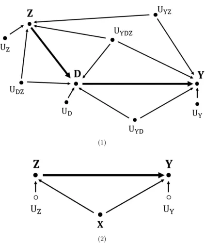
Figure A.1: Directed acyclic graph of the empirical model
(1)
(2)
Notes: A graphical representation of our empirical model in equation (1) according to Pearl (2009). Arrows denote the direction of causal relationships between variables. The top panel shows the full model and the bottom panel depicts the reduced graph when taking our identifying assumptions and perfect compliance to the instrument into consideration. Hollow circles are used to indicate unobserved variables in the reduced graph.
Figure A.2: Funding in a Virtual Common Pot
Notes: Funding status of Eurostars projects depending on their rank in the quality evaluation of a given cutoff. Black cells denote funded projects, white cells stand for projects that did not receive funding, and gray cells indicate that projects did not pass the eligibility threshold. The figure illustrates that there is sufficient variability in the funding status induced by the VCP.
Figure A.3: Overlap plots 0 1 2 3 0 .5 1 0 .5 1 Raw Matched 0 1 2 3 0 .5 1 0 .5 1 Raw Matched 0 1 2 3 0 .5 1 0 .5 1 Raw Matched
Notes: Kernel estimates of the distribution of propensity scores for the matching results in Table 3 (first graph refers to column (1) and so forth) before and after the matching. Solid line: density of the predicted probability that a funded firm is assigned to funding (fP,D=1). Dotted line: density of the predicted probability that a non-funded firm is
Figure A.4: TE heterogeneity confidence intervals -2 0 2 4 6 8 400 450 500 Score
(1) Local Linear Regression
-2 0 2 4 6 8 400 450 500 Score
(2) Fractional Polynomial Regression
A.2. Additional Tables
Table A.1: Propensity score model
(1) (2) (3) Score 0.02∗∗∗ (0.00) 0.03∗∗∗ (0.00) 0.03∗∗∗ (0.00) Employment Start 0.00 (0.00) 0.00 (0.00) 0.00 (0.00) Patent Stock 0.00 (0.00) 0.00 (0.00) 0.00 (0.00) Cutoff 2 -0.15 (0.18) -0.10 (0.19) -0.11 (0.19) Cutoff 3 0.35∗ (0.18) 0.48∗∗ (0.19) 0.47∗∗ (0.20) Cutoff 4 -0.16 (0.19) -0.09 (0.20) -0.11 (0.20) Cutoff 5 -0.05 (0.18) -0.00 (0.20) -0.03 (0.20) Cutoff 6 -0.24 (0.17) -0.26 (0.18) -0.28 (0.19) Cutoff 7 -0.50∗∗∗ (0.19) -0.39∗∗ (0.20) -0.41∗∗ (0.20) Technology Class 1 0.13 (0.17) 0.11 (0.17) 0.12 (0.17) Technology Class 2 -0.01 (0.16) -0.03 (0.17) -0.02 (0.17) Technology Class 3 -0.01 (0.18) -0.07 (0.18) -0.05 (0.18) FR 0.91∗∗∗ (0.23) 0.87∗∗∗ (0.23) IT 1.08∗∗∗ (0.25) 0.87∗∗∗ (0.30) UK, IE -0.02 (0.36) -0.09 (0.37) NL, BE, LU 0.52∗∗∗ (0.20) 0.42∗∗ (0.22) AT, CH 0.96∗∗∗ (0.25) 0.96∗∗∗ (0.25)
FI, SE, NO, DK 0.72∗∗∗ (0.18) 0.73∗∗∗ (0.18)
GR, PT, ES 0.98∗∗∗ (0.18) 0.77∗∗∗ (0.25) EU since 2004 1.22∗∗∗ (0.21) 1.12∗∗∗ (0.22) Growth Rate -9.44 (7.71) Self-funding -0.16 (0.18) Constant -9.85∗∗∗ (0.89) -12.52∗∗∗ (1.03) -12.40∗∗∗ (1.04) Observations 767 767 767
Standard errors in parentheses: ∗p <0.10,∗∗ p <0.05,∗∗∗p <0.01
Notes: Probit regression of treatment status on covariates. Fitted values are used in nearest-neighbor propensity score matching. Base categories: Germany (country groups) and Cutoff 1.
Table A.2: Nearest-neighbor Matching on Multidimen-sional Covariate Vector
(1) (2) (3)
Average Treatment Effect 0.395 0.027 0.497 (0.500) (0.476) (0.446)
Standard errors in parentheses: ∗p <0.10,∗∗p <0.05,∗∗∗p <0.01
Note: Specifications are analogous to Table 3. The Mahalanobis distance is used as metric and a bias-correction according to Abadie and Imbens (2011) is performed.
A.3. Heterogeneous Treatment Effects
Applied researchers are often interested in how treatment effects of R&D subsidies vary with other observed characteristics such as firm size or age (Czarnitzki and Lopes-Bento, 2013; Hottenrott and Lopes-Bento, 2014b,a; Balsmeier and Pellens, 2015). To explore treatment effect heterogeneity, some researchers perform a propensity score nearest-neighbor matching (PSM) and subsequently regress the difference in outcome variables of matched pairs, (Yi1−Yi,nn0 ), on a covariate of interest,W. In the following we show that it is preferable to first match on the entire covariate vector rather than the one-dimensional propensity score when using this method. We additionally perform a Monte Carlo simulation to substantiate our argument.
Let X = (X−0W, W0)0 be the entire vector of covariates and consider the setting of Section 2.1 in which we restrict attention to the region of common supportX∈S where compliance is perfect. Given the conditional independence assumption
(Y1, Y0)⊥⊥Z|X
we are able to estimate the (local) average treatment effect ofZ onY conditional on the one-dimensional propensity score (Rosenbaum and Rubin, 1983)
p(X) =P r(Z = 1|X). By the law of iterated expectations it holds that
τ =E[Y1−Y0] =E[E[Y1−Y0|p(X)]].
Consider for simplicity that all elements ofXare discrete such that exact matching is possible. Under treatment effect heterogeneity, researchers are interested in the average treatment effect conditional onW
τ(W) =E[Y1−Y0|W =w].
because τ(W = w) 6= τ(W = w0) for w 6= w0. In an exact matching on the whole covariate vector, matched pairs (asymptotically) share the same values for all elements
of X. The object of interest can then be identified as E[Y1−Y0|W =w] =EX−W E[Y1|X−W, W =w]−E[Y0|X−W, W =w] . where the expectation is taken over all elements of X excluding W. For binary W an OLS regression of the matched pairs’ differences in Y on W indeed estimates this conditional expectation.
For the propensity score matching, however, observations and their matched neighbors do not necessarily share the same values for all components ofX. The PSM only creates a control group of matched observations with the same distribution of X. Because covariates are balanced in this sense, a confounding effect ofX is eliminatedon average. But pairs matched according to the propensity score might possess very different values of W. Averaging differences for observations with W =wover the distribution ofp(X) only fixes W for the original observation and does therefore not identify the object of interest E[Y1−Y0|W = w]6=Ep(X) h p(Z = 1) E[Y1|p(X), W =w]−E[Y0|p(X)] +p(Z = 0)E[Y1|p(X)]−E[Y0|p(X), W =w] i .
For continuous covariates the same basic argument applies although exact matching is not feasible and the matching becomes less precise. Inthis case, a bias-correction pro-posed by Abadie and Imbens (2011) should be considered because matching estimators are not N1/2-consistent and contain an additional bias term that depends on the
num-ber of continuous covariates (Abadie and Imbens, 2006). In the following section, we conduct a Monte Carlo simulation to compare the performance of our proposed method with the standard procedure used in the literature.
A.4. Monte Carlo Results
Let (ε0, ε1, X1, X2) be independently standard normal. We consider two cases: (1)
W = 1(ε2 >0.5)−0.5 is binary with ε2 ∼ U(0,1), and (2) W ∼N(0,1) is continuous.
We specify treatment heterogeneity to be linear in W: τ(W) = 0.5·W + 1. Thus, the average treatment effect τ is equal to one and a linear regression should estimate the heterogeneity parameter, τ(W) = 0.5, consistently for both discrete and continuousW. We parametrize the binary treatment indicatorZ and the outcome variableY as follows Z = 1(−0.5 +W +X1−0.3·X12+ε0 >0) (3)
Y = 1 +τ(W)·Z+ exp(X1+ 0.1·X22) +X22+ε1 (4)
We compare three estimation methods to explore treatment effect heterogeneity. First, we estimate an OLS regression with interaction terms
which ignores the non-linearity in the data but serves as a benchmark. Second, we es-timate equation (3) by Probit and conduct a nearest-neighbor matching on the predicted treatment propensities. Subsequently, we regress the differences in the outcome variable Y between matched pairs onW. Third, we alter the two-step estimation by not matching firms based on the estimated propensity score but considering the Mahalanobis distance in the complete covariate vector (W, X1). Additionally, we perform a bias-correction
to improve the convergence rate of the nearest-neighbor matching (Abadie and Imbens, 2006, 2011).
Table A.3: Monte Carlo Simulation
OLS PSM NNM bias-correction: without with (1)W discrete: τ 0.642 1.015 1.015 0.846 (0.253) (0.364) (0.320) (0.356) τ(W) 0.293 0.120 0.468 0.606 (0.408) (0.430) (0.587) (0.617) (2)W continuous: τ 0.620 1.091 1.208 0.747 (0.310) (0.485) (0.295) (0.364) τ(W) 0.343 0.182 0.395 0.658 (0.214) (0.500) (0.328) (0.400)
Averaged estimation results of 200 repetitions withN = 1000. Stan-dard deviations in parentheses. (OLS): linear regression of Y on (Z, W, Z ·W, X1, X2). (PSM): propensity score matching and
sub-sequent regression of the difference in Y between matched pairs on
W. (NNM): nearest-neighbor matching on the entire covariate vector (W, X1), with and without bias-correction, and subsequent regression of
individual differences onW. Theoretical values:τ= 1 andτ(W) = 0.5.
Table A.3 presents estimated parameters averaged over 200 simulations with 1,000 observations. Nearest-neighbor matching performs best among all methods in estimating the treatment effect heterogeneity parameter. Unsurprisingly, estimations are less biased when W is discrete and exact matching is feasible. Abadie and Imbens (2006) show theoretically that the bias increases with the number of continuous covariates which is mirrored in our simulation results for continuous W. Interestingly, for our setup the bias-corrected version is further away from the true values of both the ATE and the heterogeneity parameter compared to the standard nearest-neighbor matching. The correction is based on a linear regression on the covariates (Abadie and Imbens, 2011)
which seems to harm estimation precision given the non-linear outcome model and the relatively small sample size. However, we rather regard this as a special case of our setup.
Although OLS cannot capture the non-linear part of the outcome model (equation 4) it nevertheless comes closer to the true heterogeneity parameter than the PSM method. However, point estimates for the average treatment effect τ show a large bias. In con-clusion, the PSM method performs particularly poorly in capturing the treatment effect heterogeneity, which is the main result of this simulation exercise.
FACULTY OF ECONOMICS AND BUSINESS DEPARTMENT OF MANAGERIAL ECONOMICS, STRATEGY AND INNOVATION Naamsestraat 69 bus 3500 3000 LEUVEN, BELGIË tel. + 32 16 32 67 00 fax + 32 16 32 67 32 [email protected] www.econ.kuleuven.be/MSI


![Table 3: Propensity score matching results (1) (2) (3) E[Y 1 − Y 0 |X ∈ S] 0.607 0.323 0.900 (0.490) (0.744) (0.797) Score X X X Employment Start X X X Cutoff X X X Technology X X X Patent Stock X X X Country Groups X X Growth Rate X Self-funding X Observa](https://thumb-us.123doks.com/thumbv2/123dok_us/10917307.2980716/18.892.269.626.179.491/propensity-matching-results-employment-cutoff-technology-country-observa.webp)