in
Financial Markets
DISSERTATION
zur Erlangung des Grades eines Doktors der Wirtschaftswissenschaft
eingereicht an der
Wirtschaftswissenschaftlichen Fakult¨at der Universit¨at Regensburg
vorgelegt von: Stephan Brunner
Berichterstatter:
Prof. Dr. Lutz G. Arnold (Universit¨at Regensburg)
Prof. Dr. Gerhard Illing (Ludwig-Maximilians-Universit¨at M¨unchen)
1 Introduction 1
2 Noise traders and information 5
2.1 Model setup . . . 6 2.1.1 Asset supply . . . 6 2.1.2 Asset demand . . . 9 2.1.3 Price . . . 10 2.1.4 Expectation formation . . . 10 2.1.5 Market clearing . . . 14
2.2 The transfer of wealth from noise traders to rational investors . . . 16
2.3 Expected utility . . . 19
2.4 Other distributions of the 2 ¯Z assets . . . 24
2.5 Summary . . . 28
2.A Calculations . . . 30
2.B Alternative decompositions of the final wealth . . . 32
2.C Mathematica source code . . . 37
3 Positive Feedback Traders 47 3.1 Model . . . 48
3.2 Investment behavior . . . 51
3.3 Case with one signal . . . 57
3.3.1 Destabilizing rational speculation (the DSSW Model) . . . 57
3.3.3 Neutral rational speculation . . . 62
3.3.4 The general case . . . 63
3.3.5 The effect of measure in the presence of rational speculators . . 71
3.3.6 The effect of measure in the absence of rational speculators . . . 75
3.3.7 Fundamental value and bubbles . . . 76
3.4 Case with two signals . . . 82
3.4.1 The general case . . . 82
3.4.2 Setup 1 . . . 87
3.4.3 Setup 2 . . . 92
3.4.4 Setup 3 . . . 100
3.4.5 The possibility of non-existence of an equilibrium . . . 103
3.4.6 Price behavior in the absence of rational speculators . . . 104
3.4.7 Uniqueness . . . 109
3.4.8 Bubbles . . . 126
3.5 Results . . . 130
2.1 Initial and final asset allocation for different realizations of Z. . . 7
2.2 Expected utility for type-A agents . . . 22
2.3 Expected utility for type-B agents . . . 24
2.4 Expected utility for type-A and type-B agents . . . 25
2.5 Initial and final asset allocation for different realizations of Z. . . 26
3.1 Destabilizing speculation . . . 57
3.2 Stabilizing speculation . . . 60
3.3 Neutral speculation . . . 62
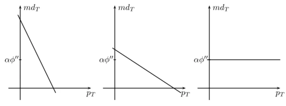
3.4 The market demand . . . 73
3.5 The three different time setups. . . 87
3.6 Determination of λ0 and ν0 . . . 88
3.7 Possible prices reactions . . . 91
3.8 Shape of the denominator and of (3.34). . . 94
3.9 Shape of the numerator of the slope and of (3.35) . . . 96
3.10 Determination of ν0 and λ0 in the case IIB and in the case IIA. . . 99
3.11 Possible price pathes for λ0 <0< ν0 and 0< λ0 < ν0. . . 100
3.12 Shape of the numerator of the intercept and the intercept. . . 101
The present work focuses on the role of noise traders in financial markets. First and foremost, this task requires to define the term noise traders. There is a broad variety of definitions for noise traders in the literature (see Dow & Gorton (2006)). Subsequently, we adopt the two definitions of noise traders by Kyle (1985) and De Long et al. (1990). In chapter 2 we characterize noise traders as agents who trade randomly, whereas we describe them as agents who choose their demand dependent on past price changes in chapter 3.
Before taking a closer look at the behavior of noise traders, we discuss the role of noise in financial markets. Following Grossman (1976), noise is needed to solve the no trade argument put forward by Migrom & Stokey (1982). By this argument a market agent, even though he has additional private information, cannot profit from it. An agent with superior information is interested in buying an asset if the value of the asset, conditional on his information, exceeds its price. Thus, the price which is offered by the buyer is smaller than or equal to the value of the asset. The seller, who does not have additional information on the asset, knows that the buyer would not demand the asset if the price exceeded its value. Hence, no one trades since the seller is not worse off if he keeps the asset.
A formal framework for that issue is a Rational Expectations Equilibrium (REE) model. Agents in an REE model fully understand the model economy and the market mech-anisms. If an informed agent uses his information for trading, it has an influence on the price. Therefore also uninformed agents learn from that information since they can deduce informed agents’ information from the price. The price that forms in
equilib-rium reflects all information in the market. If information is costly, then no one has an incentive to gather information since the price already incorporates the “best” available information (see Grossman (1976)). One way to give informed agents the possibility to benefit from their additional information is the implementation of noise, for example via a stochastic asset supply (brought forward in Grossman (1976)). The price in this setup is not fully, but only partially revealing the information of informed agents. This idea of a noisy asset supply is also used in models by Grossman & Stiglitz (1980) and Hellwig (1980) which we adopt in the first section of this dissertation. The random supply, however, will be interpreted as the outcome of noise traders. Following Kyle (1985), it is assumed that these noise traders trade randomly and independently from the price. We will examine how noise traders perform in the market (via expected final wealth) and how different model parameters affect their performance. The definition of noise traders adopted here was used by Gloston & Milgrom (1985) as well, who explain the random trading behavior of noise traders by exogenous shocks like job losses or promotions. This definition of noise traders is worth a discussion which is outlined in section 2.5.
A result of chapter 2 is that noise traders’ expected total wealth is decreasing. If noise traders performance is on average “bad” it gives rise to the question why they should survive in the market. One explanation is that arbitrage opportunities are limited. Reasons for that could be a limited time horizon (Dow & Gorton (1994)) or professional market agents (Shleifer & Vishny (1997) and Arnold (2009)). Nonetheless, section 2 does not focus on that issue since we consider a two-period model and not a long time horizon.
Since the learning process of market agents and the price formation in a REE model occur simultaneously, strategic behavior is absent. We will analyze an example for strategic behavior in the second part of this work by extending the model of De Long et al. (1990) (henceforth: DSSW) who introduce positive feedback traders. These are market agents that determine their demand by observing past price changes. If the price increased in the past, they demand the asset, if it decreased, they sell it. There may be different reasons for that behavior: it may come for example “from
extrapol-ative expectations about prices, or trend chasing” (Shleifer, 2000, p.155). A rational agent can exploit this behavior: if he receives a positive signal about the future pay-off, he knows that the price will increase tomorrow. This price increase will lead to a future positive demand of positive feedback traders. Anticipating this positive de-mand, rational agents will drive the prices even to a higher level and then sell the asset tomorrow. The presence of rational agents therefore has a rather destabilizing than stabilizing effect on the price. In section 3 we present an extension of the DSSW model by applying another time structure and adding a second signal.
The aim of this section is to analyze the performance of noise traders by considering their expected final wealth. We will see that the amount of expected wealth that noise traders lose is gained by rational agents. Hence, there is a transfer of expected wealth from noise traders to rational agents. Interestingly, this transfer decreases as the fraction of informed agents in the market increases.
For the remainder of this chapter we follow Kyle (1985) and describe noise traders as agents who randomly purchase or sell assets no matter what the price of the asset is. Their behavior can be explained by exogenous shocks (see Gloston & Milgrom (1985)). Since we do not assume a specific utility function for noise traders, our measure of how good or how bad they perform is the expected value of their final wealth. The only assumption we make is that a higher expected wealth is better for them.
In section 2.1 we present our model following Grossman & Stiglitz (1980) and Hellwig (1980). After that, we are in the position to give an expression for the expected transfer of wealth from noise traders to rational agents (section 2.2). We also examine the effect of different parameters on the expected final wealth. In section 2.3 we take a look at the expected utility of rational agents. The results there are in line with Grossman & Stiglitz (1980). Another distribution of the initial wealth will be discussed in section 2.4.
2.1 Model setup
The model we use is a modified version of the partially revealing REE model used by Grossman & Stiglitz (1980) with the notation of Hellwig (1980). There is a continuum of agents on the interval [0,1]. Following Grossman & Stiglitz (1980) and Hellwig (1980), agents can allocate their initial wealth to one riskless and one risky asset, where the former pays one unit and the latter X units of a single consumption good. Let p denote the price of the risky asset and take the riskfree asset to be numeraire. The initial endowment of agent i consists of a constant part w0i and a given amount
¯
Z of the risky asset. The final wealth of agent i holdingzi units of the risky assets is
given by
w1i =w0i+pZ¯+zi(X−p). (2.1)
Following Grossman & Stiglitz (1980), we assume that agents maximize their expected utility E[U], with
U =−e−ρw1i,1
where ρ is a parameter for absolute risk aversion.
2.1.1 Asset supply
According to both papers cited above, we assume that the supply is risky. We explain this random supply by noise traders. Given a fixed amount of 2 ¯Z assets where one half (= ¯Z) is held by the agents we introduced above (RAT) and the other half (= ¯Z) is possessed by agents we call noise traders (NT) (upper panel of figure 2.1). As already stated in the beginning of this chapter, noise traders are hit by exogenous shocks and therefore randomly2 buy or sell the asset. The total supply of noise traders is given by
1The choice of this specific utility function (CARA) used by Grossman and Stiglitz (1980) is consistent
with assumption A1 in (Hellwig, 1980, p.479).
2On the one hand side there are noise traders that demand the asset. On the other hand side some
noise traders sell it. We are just interested in the overall reaction of noise traders. Also note, that noise traders are not interested in the price of the asset. They just sell or purchase the asset.
rational investors noise traders
0 Z¯ 2 ¯Z
rational investors noise traders
0 Z Z¯ 2 ¯Z
Z −Z <¯ 0
rational investors noise traders
0 Z¯ Z 2 ¯Z
Z −Z >¯ 0
Figure 2.1: Initial (top) and final (middle and bottom) asset allocation for two different realizations of Z
Z−Z¯ ∼N(0,∆2). Hence, on average the amount of assets supplied or demanded by
noise traders is zero. In the case of a positive realization ofZ −Z¯ (see lower panel of figure 2.1) noise traders sell part of their assets, whereas ifZ−Z¯is negative (see middle panel of figure 2.1) they purchase assets. Therefore, the total (stochastic) supply of assets for rational agents is given by
¯ Z
|{z}
assets held by RAT
+ (Z−Z¯)
| {z }
total supply of NT
=Z ∼N( ¯Z,∆2).3
Recall that we refrain from using a specific utility function for noise traders and instead consider their final wealth
w1,N T = Z¯−(Z−Z¯)
| {z }
assets held by NT at date 1
X+ Z−Z¯
| {z }
assets NT sold to/bought from RAT p
= XZ¯−(Z−Z¯)(X−p),
3By assuming that ¯Z is “large enough” we can neglect the cases where the total supply is negative.
which depends on the realizations of the payoff X and the supplyZ. Hence, expected wealth is E[w1,N T] = E[XZ¯−(Z−Z¯)(X−p)] = X¯Z¯−E[(Z−Z¯)(X−p)] = X¯Z¯−E[(Z−Z¯)]E[(X−p)]−Cov[Z−Z, X¯ −p] = X¯Z¯−( ¯Z−Z¯)E[(X−p)]−Cov[Z −Z, X¯ −p] = X¯Z¯−Cov[Z−Z, X¯ −p].
Note, that the expected wealthE[w1,N T] is decreasing in the covariance betweenZ−Z¯
and X−p.4 If the covariance is not equal to zero there is a transfer of expected wealth
from noise traders to rational agents. To verify this, we consider the expected total final wealth of rational agents. Recall that the final wealth of a rational agent is
w1i =w0i+pZ¯+zi(X−p).
The total final wealth of all rational agents in equilibrium is therefore
w1,RAT =w0+pZ¯+Z(X−p), wherew0 = 1 R 0 w0i diand 1 R 0
zi di=Z.5Hence, the expected total final wealth of rational
agents is E[w1,RAT] = E[w0+ ¯Zp+Z(X−p)] = E[w0+ ¯ZX+ (Z−Z¯)(X−p)] = w0+ ¯ZX¯ +E[(Z−Z¯)(X−p)] = w0+ ¯ZX¯ +E[Z−Z¯]E[X−p] +Cov[Z−Z, X¯ −p] = w0+ ¯ZX¯ +Cov[Z −Z, X¯ −p].
So, in contrast to noise traders’ expected wealth, the expected wealth of rational agents is increasing in the covariance betweenZ−Z¯ andX−p. Note, that the total expected
4This is also true for alternative partitions of the 2 ¯Z assets among NT and RAT (see section 2.4). 5This is the market clearing condition we will specify later.
wealth of both groups is
E[w1,N T] +E[w1,RAT] = X¯Z¯−Cov[Z−Z, X¯ −p] +w0+ ¯ZX¯ +Cov[Z−Z, X¯ −p]
= w0+ 2 ¯ZX¯
which is the constant initial wealth of rational agents w0 plus the total of assets 2 ¯Z
multiplied by the expected value ¯X. This means that the amount of expected wealth which noise traders lose is gained by rational agents and vice versa. The following table gives an overview over the initial and final holdings and the corresponding wealth.
rational speculators noise traders total
initial holdings Z¯ Z¯ 2 ¯Z
initial wealth w0+pZ¯ pZ¯ w0+ 2pZ¯
final holdings Z¯+ (Z−Z¯) = Z Z¯−(Z −Z¯) = 2 ¯Z−Z 2 ¯Z final wealth w0+XZ¯+ (X−p)(Z−Z¯) XZ¯−(X−p)(Z−Z¯) w0+ 2XZ¯
In order to specify the covariance (and therefore the transfer of wealth) more precisely, we will now continue with the presentation of the model.
2.1.2 Asset demand
We subdivide rational agents into two groups: a fraction of 1−τ type-A agents and a fraction ofτ type-B agents. We will use the superscriptsA and B to indicate that the parameter refers to the corresponding agent.6 Both types of agents use information
to rationally form expectations of the future payoff of the risky asset. Heterogeneity among the two groups of agents is induced by the amount of information they use. Specifically, we assume that type-A agents are only able to learn from the price, whereas type-B agents additionally have the ability to process7 a private signal yi = X +i,
6Type-A agents correspond to the uninformed agents in Grossman & Stiglitz (1980), type-B agents
to informed agents.
7We refrain from introducing costs for gathering information as in Grossman & Stiglitz (1980). In
wherei ∼N(0, σ2) ∀i. Therefore, the individual demand of type-A and type-B agents is8 zAi = E[X|p]−p ρV ar[X|p] (2.2) and ziB = E[X|p, yi]−p ρV ar[X|p, yi] . (2.3)
2.1.3 Price
Before taking a closer look at the expectations of the two types of agents, we have to consider the price. For given information, agents derive their expectation of X based on p (type A) and p and yi (type B), respectively. As outlined in Hellwig (1980),
“expectations formation and market clearing cannot be treated separately” (Hellwig, 1980, p.480). When agents form their expectations, they consider the price of the asset. The expectations influence the market clearing condition and therefore the price. Thus, expectations formation and market clearing must be considered simultaneously. This is a fixed-point problem that has a linear solution. Following Hellwig (1980), we first assume that the price is linear in X and Z, i.e.
p=π0+π1X−γZ, (2.4)
whereπ0,π1 andγ are constant. Using this assumption, we will see later that the price
is in fact a linear combination ofX and Z. Anticipating the form of the price function, we can now take a closer look at the expectations on X of the two different types of agents.
2.1.4 Expectation formation
Agents of type A
As stated above, type-A agents form their expectations conditional only on the price.
The variance-covariance-matrix of the normal vector X p with mean ¯ X π0+π1X¯ −γZ¯ is given by VA= σ2 X π1σ2X π1σX2 π12σ2X +γ2∆2 .
Therefore, following Raiffa & Schlaifer (1961), the conditional distribution of X given pis also normal with mean
E[X|p] =α0Ai+αA2ip (2.5) and varianceV ar[X|p] =βA
i .9 Since, by assumption, all agents of type A are identical
the subscripti can be omitted. Specifically,
E[X|p] = X¯+ π1σ 2 X π2 1σ2X +γ2∆2 (p−π0−π1X¯ +γZ¯) = π 2 1σX2X¯ +γ2∆2X¯ −π0π1σ2X −π21σX2X¯+π1γσX2Z¯ π2 1σX2 +γ2∆2 + π1σ 2 X π2 1σ2X +γ2∆2 p = γ 2∆2X¯ −π 0π1σX2 +π1γσX2Z¯ π2 1σX2 +γ2∆2 + π1σ 2 X π2 1σX2 +γ2∆2 p 9Let (X, S)
∼N(µ,Σ) be a n−dimensional random variable with µ= µX µS and Σ = ΣX,X ΣX,S ΣS,X ΣS,S . Then (X|S=s)∼NµX+ ΣX,SΣ−S,S1(s−µS),ΣX,X −ΣX,SΣ−S,S1ΣS,X . (2.6) (Raiffa & Schlaifer, 1961, p.250).
and V ar[X|p] = σX2 − π 2 1σX4 π2 1σX2 +γ2∆2 = π 2 1σ4X +γ2∆2σX2 −π12σX4 π2 1σ2X +γ2∆2 = γ 2∆2σ2 X π2 1σ2X +γ2∆2 = βA. (2.7) Therefore, αA0 = γ 2∆2X¯ −π 0π1σ2X +π1γσ2XZ¯ π2 1σX2 +γ2∆2 (2.8) and αA2 = π1σ 2 X π2 1σX2 +γ2∆2 . (2.9) Agents of type B
In contrast to type-A agents, agents of type B form their expectation of the payoff dependent not only on the price p but also conditional on a private signal yi. Hence,
the conditional expectation given pand yi is
E[X|yi, p] =αB0i+α B
1iyi+αB2ip (2.10)
with varianceV ar[X|yi, p] =βiB. Since we assume that the private signal has the same
variance for all agents of type B, the subscriptiatαB
0i,αB1i,αB2i, andβiB can be omitted.
The variance-covariance matrix of the normal vector
X yi p with mean ¯ X ¯ X π0+π1X¯ −γZ¯ is VB = σ2 X σ2X π1σX2 σX2 σX2 +σ2 π1σX2 π1σ2X π1σX2 π12σX2 +γ2∆2 .
Following again Raiffa & Schlaifer (1961), E[X|yi, p] and V ar[X|yi, p] are given by10 E[X|yi, p] = X¯ + σ2X π1σX2 σ2 X +σ2 π1σX2 π1σ2X π21σX2 +γ2∆2 −1 yi−X¯ p−π0−π1X¯ +γZ¯ = X¯ + 1 (σ2 X +σ2)(π12σX2 +γ2∆2)−π12σX4 σ2 X π1σX2 π2 1σX2 +γ2∆2 −π1σX2 −π1σX2 σX2 +σ2 yi−X¯ p−π0−π1X¯ +γZ¯ = X¯ + 1 σ2 γ2∆2+σ2X(π21σ2+γ2∆2) σX2(π12σ2X +γ2∆2)−π12σX4 −π1σ4X +π1σX2 (σX2 +σ2) t yi−X¯ p−π0−π1X¯+γZ¯ = X¯ − γ 2∆2σ2 XX¯ +π1σX2 σ2(π0+π1X¯ −γZ¯) σ2 γ2∆2+σX2(π12σ2 +γ2∆2) + γ 2∆2σ2 X σ2 γ2∆2+σ2X(π21σ2+γ2∆2) yi + π1σ 2 Xσ2 σ2 γ2∆2+σ2X(π21σ2+γ2∆2) p and V ar[X|yi, p] = σ2X − σ2 X π1σX2 σX2 +σ2 π1σX2 π1σ2X π21σX2 +γ2∆2 −1 σX2 π1σX2 = σ2X − γ2∆2σ2X σ2 γ2∆2+σ2X(π21σ2+γ2∆2) π1σ2Xσ2 σ2 γ2∆2+σX2(π21σ2+γ2∆2) σX2 π1σ2X = γ 2∆2σ2 Xσ2 σ2 γ2∆2+σ2X(π21σ2+γ2∆2) = βB. (2.11) 10 a b c d −1 = ad1−bc d −b −c a
Therefore, αB0 = X¯ − γ 2∆2σ2 XX¯ +π1σX2σ2(π0+π1X¯ −γZ¯) σ2 γ2∆2+σX2(π21σ2 +γ2∆2) = γ 2∆2σ2 X¯ −π0π1σX2σ2+γπ1σX2σ2Z¯ σ2 γ2∆2+σX2(π12σ2 +γ2∆2) , (2.12) αB1 = γ 2∆2σ2 X σ2 γ2∆2+σX2(π12σ2 +γ2∆2) (2.13) and αB2 = π1σ 2 Xσ2 σ2 γ2∆2+σ2X(π12σ2+γ2∆2) . (2.14)
2.1.5 Market clearing
Given the demand of both types of agents zA
i and zBi and the supply Z of the asset,
market clearing requires
Z = τ Z 0 ziB di+ 1 Z τ ziA di.
Note, that since agents of type A all have the same information about the future payoff (i.e. the price)
1
R
τ
ziA di= (1−τ)ziA.
Using (2.2), (2.3), (2.5), and (2.10) the market clearing condition becomes
Z = (1−τ)E[X|p]−p ρβA + τ Z 0 E[X|yi, p]−p ρβB = (1−τ)α A 0 + (α2A−1)p ρβA +τ αB 0 +αB1X+ (αB2 −1)p ρβB = (1−τ)α A 0βB+τ αB0βA+ (1−τ)(α2A−1)βB+τ(αB2 −1)βA p+τ αB 1βAX ρβAβB .
Solving for p, we get
p = − (1−τ)α A 0βB+τ αB0βA (1−τ)(αA 2 −1)βB+τ(αB2 −1)βA − τ α B 1βA (1−τ)(αA 2 −1)βB+τ(αB2 −1)βA X + ρβ AβB (1−τ)(αA 2 −1)βB+τ(αB2 −1)βA Z.
Hence, π0 =− (1−τ)αA0βB+τ αB0βA (1−τ)(αA 2 −1)βB+τ(αB2 −1)βA , π1 =− τ αB 1βA (1−τ)(αA 2 −1)βB+τ(αB2 −1)βA and γ =− ρβ AβB (1−τ)(αA 2 −1)βB+τ(αB2 −1)βA .
It can be seen that a linear price in X and Z actually solves our problem.
Plugging (2.7), (2.8), (2.9), (2.11), (2.12), (2.13), and (2.14) in the three preceding equations we get11 π0 = (1−τ)αA 0βB+τ αB0βA (1−τ)(1−αA 2)βB+τ(1−α2B)βA = σ 2 γ2∆2X¯+π1σX2 γZ¯−π0 γ2∆2σ2 +σX2 (γ2∆2τ+ (π1−1)π1σ2) , (2.15) π1 = τ αB 1βA (1−τ)(1−αA 2)βB+τ(1−αB2)βA = γ 2∆2τ σ2 X γ2∆2σ2 +σX2 (γ2∆2τ + (π1−1)π1σ2) (2.16) and γ = ρβ AβB (1−τ)(1−αA 2)βB+τ(1−αB2)βA = γ 2∆2ρσ2 Xσ2 γ2∆2σ2 +σ2X(γ2∆2τ + (π1 −1)π1σ2) . (2.17)
Solving (2.15) forπ0 leads to
π0 = γσ2 γ∆2X¯ +π1Zσ¯ X2 γ2∆2σ2 +σX2 (γ2∆2τ+π12σ2) . (2.18)
We have to solve equations (2.16) and (2.17) simultaneously because both contain γ and π1. Since the right hand sides in both equations have the same denominator we
get12 γ2∆2ρσX2σ2 γ = γ2∆2τ σX2 π1 ⇔γ2∆2ρσX2σ2π1 = γ2∆2ρσX2 σ 2 γ ⇔γ = ρσ 2 π1 τ . (2.19)
Plugging (2.19) in (2.16) and solving for π1 (see appendix 2.A) we get
π1 =
τ σ2X(∆2ρ2σ2+τ) ∆2ρ2σ4
+τ σX2 (∆2ρ2σ2+τ)
. (2.20)
Using this together with (2.19) we obtain
γ = ρσ 2 τ τ σ2X(∆2ρ2σ2 +τ) ∆2ρ2σ4 +τ σX2 (∆2ρ2σ2+τ) = ρσ 2 Xσ2(∆2ρ2σ2 +τ) ∆2ρ2σ4 +τ σX2 (∆2ρ2σ2+τ) . (2.21)
Finally, we can plug π1 and γ in equation (2.18) yielding
π0 = ρσ2 ∆2ρXσ¯ 2 +τZσ¯ X2 ∆2ρ2σ4 +τ σX2 (∆2ρ2σ2+τ) . (2.22)
2.2 The transfer of wealth from noise traders to
rational investors
In section 2.1.1 we have shown that the expected value of the final wealth is
E[w1,RAT] =w0+ ¯ZX¯ +Cov[Z−Z, X¯ −p]
for rational agents and
E[w1,N T] = ¯ZX¯ −Cov[Z−Z, X¯ −p]
for noise traders. Hence, the transfer of expected wealth from noise traders to rational agents is exactly the covariance betweenZ−Z¯ andX−p. Since we have specified the
12Note, thatπ
0=γ= 0 also solves (2.19). However, this does not solve equations (2.16) and (2.17)
price function and its parameters, we are now in the position to calculate the covariance Cov[Z−Z, X¯ −p] = Cov[Z, X−π0−π1X+γZ] = Cov[Z, γZ] = γ∆2 = ρσ 2 Xσ2∆2(∆2ρ2σ2 +τ) ∆2ρ2σ4 +τ σX2 (∆2ρ2σ2+τ) ,
since ¯Z is constant and X and Z are uncorrelated. This covariance is in fact always positive since ρ >0, τ ∈[0,1], and all variances are positive. Therefore, noise traders lose expected wealth and this is actually transferred to rational speculators. To un-derstand that, we compare the final wealth for realizations Z > Z¯ and Z < Z¯ and compare it to the case when the realization ofZ is equal to ¯Z. Recall that the price is
p=π0+π1X−γZ.
Since γ >0, the price increases as Z decreases and vice versa. Consider that we have realizations Z and X. If Z > Z¯, noise traders overall sell assets (actually Z −Z >¯ 0 assets). This increased supply to rational agents decreases (compared to Z = ¯Z) the price viaγ. Thus the rational agents buy a positive amountZ−Z¯ for a “lower” price. If in contrast Z < Z¯, noise traders demand the asset (exactly ¯Z −Z assets) and the reduced supply to rational agents increases the price via γ (again compared to the realization Z = ¯Z). Thus, rational agents sell the asset at a “higher” price. In both cases rational agents are better off than in the case when the realization of Z is ¯Z. This explains why rational agents’ expected wealth (lessw0) is always larger than noise
traders’ expected wealth.
In the following we examine the effect of the different parameters on the variance. We therefore differentiate γ∆2 with respect to the corresponding parameter.
The influence of σ2
X on the transfer of wealth
Considering ∂(γ∆2) ∂σ2 X = ρσ 2 ∆2(∆2ρ2σ2+τ) (∆2ρ2σ4+τ σX2 (∆2ρ2σ2+τ)) (∆2ρ2σ4 +τ σX2 (∆2ρ2σ2+τ)) 2 −ρσ 2 Xσ2∆2(∆2ρ2σ2+τ)τ(∆2ρ2σ2+τ) (∆2ρ2σ4 +τ σX2 (∆2ρ2σ2+τ)) 2 = ρ 3∆4σ6 (∆2ρ2σ2+τ) (∆2ρ2σ4 +τ σX2 (∆2ρ2σ2+τ)) 2 >0,
we see that the transfer of wealth is increasing in the variance of X. We have seen in the price function that the future payoffX of the asset has an impact on the price. An increase in σ2
X decreases the price since the price incorporates more risk. Hence, the
price decreases such that noise traders are paid worse for the assets they sell.
The influence of ∆2 on the transfer of wealth
Next, we study the effect of an increased variance in the supply on the expected wealth of noise traders. The derivative of γ∆2 with respect to ∆2 is
∂γ∆2 ∂∆2 = (∆2ρ2σ4 +τ σ2X(∆2ρ2σ2+τ)) (2∆2ρ3σX2 σ4 +τ ρσ2Xσ2∆2) (∆2ρ2σ4 +τ σX2 (∆2ρ2σ2+τ)) 2 −(ρ 2σ4 +τ σ2Xρ2σ2)ρσ2Xσ2∆2(∆2ρ2σ2+τ) (∆2ρ2σ4 +τ σ2X(∆2ρ2σ2 +τ)) 2 = ∆ 4ρ5σ2 Xσ8 +ρτ σ4Xσ2(∆2ρ2σ2+τ)2 (∆2ρ2σ4 +τ σ2X(∆2ρ2σ2+τ)) 2 >0.
Here happens the same as in the case when the variance of the payoff increases. An increase in ∆2 increases the risk that is incorporated in the price. This decreases the price and therefore noise traders sell their assets at a cheaper price. So their expected wealth decreases in ∆2.
The influence of τ on the transfer of wealth
The last issue to analyze is the effect of τ on the expected wealth of noise traders. Therefore, we consider ∂γ∆2 ∂τ = (∆2ρ2σ4+τ σX2 (∆2ρ2σ2+τ))ρσX2σ2∆2 (∆2ρ2σ4 +τ σ2X(∆2ρ2σ2 +τ)) 2 −(τ ρ 2σ2 X∆ 2σ2 + 2τ σX2)ρσ 2 Xσ 2 ∆2(∆2ρ2σ2+τ) (∆2ρ2σ4 +τ σX2 (∆2ρ2σ2+τ)) 2 = −∆ 2ρσ2 Xσ2(σX2 (∆2ρ2σ2+τ)2−∆2ρ2σ4) (∆2ρ2σ4 +τ σX2 (∆2ρ2σ2 +τ)) 2 .
This derivative is negative if and only if
σ2X ∆2ρ2σ2 +τ2−∆2ρ2σ4 >0⇔σX2 ∆2ρ2σ2+τ2 >∆2ρ2σ4. The function
σX2 ∆2ρ2σ2+τ2
−∆2ρ2σ4
is a upward open parabola inτ which is monotonically increasing for τ > 0 since the apex (−∆2ρ2σ2,−∆2ρ2σ4) is in the third quadrant. Therefore, it is sufficient to show that the function is positive forτ = 0. In that case we have
σ2X∆4ρ4σ4 −∆2ρ2σ4 >0⇔σX2∆2ρ2 >1.
If we assume that the latter inequality holds,13 the transfer of wealth decreases as τ
increases. So the higher the fraction of informed investors ( = investors that learn from the price and a private signal (type-B)) in the market, the lower is the transfer of wealth from noise traders to rational agents. At first sight one might think that the other way round is true: the more informed rational agents, the better the opportunities for them to exploit noise traders. The reason why that is not the case is the following: if the number of type-B agents increases, the price incorporates more information and less risk. This decline of risk increases the price. Therefore noise traders get a higher price for their assets.
2.3 Expected utility
For completeness, we also consider the expected utility of rational agents similar as in Grossman & Stiglitz (1980). As stated in the model presentation, agents are maxim-izing their expected utility. Recall, that
U =−e−ρw1i =−e−ρ(w0i+ ¯Zp+zi(X−p)).
Sincezi and X−pare normally distributed, the exponent of U contains a product of
two normal distributed random variables. Following Brunnermeier (2001) we compute expected utility by using the following lemma:
Lemma 1. Let w ∼ N(0,Σ) be a multinomial random variable with positive definite variance-covariance-matrix. Then E[ewtAw+btw+d] =|I−2ΣA|12e 1 2(I−2ΣA) −1Σb+d ,
where I is the identity matrix, A is a symmetric matrix, b a vector, d a scalar, and |.| the determinant (Brunnermeier, 2001, p.64).
The expected utilities of both types of agents have to be derived separately because the amount of shares held by agents of type A and type B are different.
Agents of type A
In order to apply lemma 1, w1i has to be brought in the appropriate form:
w1i = w0i+ziA(X−p) + ¯Zp = w0i+ (ziA−z¯ A i )(X−p) + ¯z A i (X−p) + ¯Z(p−p¯) + ¯Zp¯ = w0i+ (ziA−z¯ A i )(X−p−( ¯X−p¯)) + (z A i −z¯ A i )( ¯X−p¯) +¯ziA(X−p−( ¯X−p¯)) + ¯ziA( ¯X−p¯) + ¯Z(p−p¯) + ¯Zp¯ = zA i −z¯iA X−p−( ¯X−p¯) p−p¯ 0 12 0 1 2 0 0 0 0 0 zA i −z¯iA X−p−( ¯X−p¯) p−p¯ + X¯ −p¯ z¯A i Z¯ zA i −z¯iA X−p−( ¯X−p¯) p−p¯ +w0i+ ¯ziA( ¯X−p¯) + ¯Zp¯ (2.23)
where ¯ziA, ¯X, and ¯pare the means of ziA, X, and p. Using
A= 0 −ρ2 0 −ρ 2 0 0 0 0 0 , b= −ρ( ¯X−p¯) −ρz¯iA −ρZ¯ ,
d=−ρ w0i+ ¯ziA( ¯X−p¯) + ¯Zp¯ , and Σ = σz2A i Cov[z A i , X −p] Cov[ziA, p] Cov[zA i , X−p] σX2−p Cov[X−p, p] Cov[zA i , p] Cov[X−p, p] σp2
we are able to calculate the expected utility.14 The final thing to determine are the
entries in the matrix Σ which are
σz2A i = V ar αA 0 + (αA2 −1)(π0+π1X−γZ) ρβA = (αA 2 −1)π1 ρβA 2 σX2 + (αA 2 −1)γ ρβA 2 ∆2, Cov[ziA, X −p] = Cov αA 0 + (αA2 −1)(π0+π1X−γZ) ρβA , X −π0−π1X+γZ = (α A 2 −1)π1 ρβA (1−π1)σ 2 X − (αA2 −1)γ2 ρβA ∆ 2, Cov[ziA, p] = Cov αA 0 + (αA2 −1)(π0+π1X−γZ) ρβA , π0+π1X−γZ = (α A 2 −1)π21 ρβA σ 2 X + (αA 2 −1)γ2 ρβA ∆ 2, σX2−p = V ar[X−π0−π1X+γZ] = (1−π1)2σ2X +γ 2∆2, Cov[X−p, p] = Cov[X−π0−π1X+γZ, π0+π1X−γZ] = (1−π1)π1σ2X −γ 2∆2 and σp2 = V ar[π0+π1X−γZ] = π12σX2 +γ2∆2.
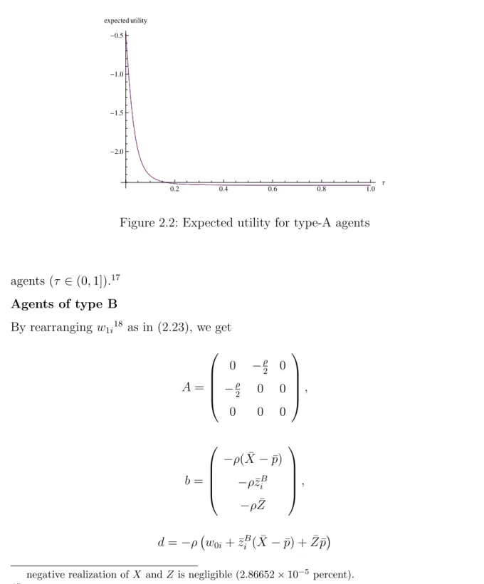
For the ease of exposition we plot (see figure 2.2)15the expected utility for the example16
ρ= 5, σX = 1, X¯ = 5, Z¯ = 5, ∆ = 1, σ = 101 , and w0 = 1 over the fraction of type-B 14Note, that another decomposition is also possible. To check that the results are correct we used
another decomposition with the variable vector X−X¯ Z−Z¯
t
(see appendix 2.B).
15Figures 2.2, 2.3, and 2.4 were produced using Wolfram Mathematica. The source code can be found
in appendix 2.C.
0.2 0.4 0.6 0.8 1.0 Τ -2.0 -1.5 -1.0 -0.5 expected utility
Figure 2.2: Expected utility for type-A agents
agents (τ ∈(0,1]).17 Agents of type B By rearranging w1i18 as in (2.23), we get A= 0 −ρ2 0 −ρ2 0 0 0 0 0 , b= −ρ( ¯X−p¯) −ρz¯B i −ρZ¯ , d =−ρ w0i+ ¯ziB( ¯X−p¯) + ¯Zp¯
negative realization ofX andZ is negligible (2.86652×10⁻⁵ percent).
17The expected utility drops very steeply at the beginning for small values ofτ. The reason for that is
that the variance of the signal is very small. Ifσ2
increases, the expected utility function becomes
flatter since the price does not become informative “so fast”. This is in line with the results in Grossman & Stiglitz (1980) since “[a]n increase in the quality of information [...] increases the informativeness of the price system” (Grossman & Stiglitz, 1980, p.399).
18We also checked the results with another decomposition where the normal vector was
X−X¯ Z−Z¯ i t
and Σ = σ2 zB i Cov[zB i , X −p] Cov[ziB, p] Cov[zB i , X−p] σ2X−p Cov[X−p, p] Cov[zB i , p] Cov[X−p, p] σp2 .
The entries in the matrix Σ are
σ2zB i = V ar αB 0 +αB1(X+i) + (αB2 −1)(π0+π1X−γZ) ρβB = αB 1 + (αB2 −1)π1 ρβB 2 σX2 + (αB 2 −1)γ ρβB 2 ∆2+ αB 1 ρβB 2 σ2, Cov[ziB, X −p] = Cov αB 0 +α1B(X+i) + (α2B−1)(π0+π1X−γZ) ρβB , X−π0−π1X+γZ] = α B 1 + (αB2 −1)π1 ρβB (1−π1)σ 2 X − (αB 2 −1)γ ρβB γ∆ 2, Cov[ziB, p] = Cov αB0 +α1B(X+i) + (α2B−1)(π0+π1X−γZ) ρβB , π0+π1X−γZ] = α B 1 + (αB2 −1)π1 ρβB π1σ 2 X + (αB2 −1)γ ρβB γ∆ 2 , σ2X−p = V ar[X−π0−π1X+γZ] = (1−π1)2σX2 +γ 2 ∆2, Cov[X−p, p] = Cov[X−π0−π1X+γZ, π0+π1X−γZ] = (1−π1)π1σX2 −γ 2 ∆2, and σp2 = V ar[π0+π1X−γZ] = π12σX2 +γ2∆2.
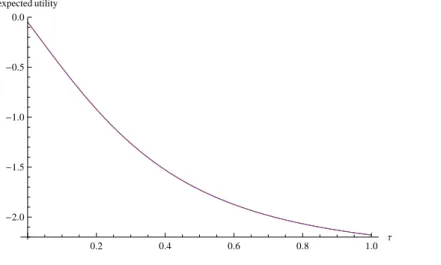
Again, the expected utility is plotted as a function of τ using the same parameters as in the previous paragraph (figure 2.3).
Comparison of type-A and type-B agents
When we draw both expected utility functions in a E[U]−τ−diagram (figure 2.4), we see that agents who are able to process additional information (type B) are always
0.2 0.4 0.6 0.8 1.0 Τ -2.0 -1.5 -1.0 -0.5 0.0 expected utility
Figure 2.3: Expected utility for type-B agents
better off compared to agents who form their expectations using only the price (type A). This is different to the model of Grossman & Stiglitz (1980). The reason is that we do not consider costs of information for type-B agents. We assume that some agents have the ability to process information whereas others have not. If we introduced costs of information, the upper curve would be shifted downwards and, hence, there would exist a point where the expected utilities of both groups are identical.
Although rational agents’ expected wealth is increasing in τ (see sections 2.1.1 and 2.2), their expected utility is decreasing in our example for both groups of rational agents. As τ increases, the number of agents that additionally learn from a private signal is increasing. If there are more agents who can process information then the price contains more information and rather reflects the future value X of the asset. Therefore, the price becomes more appropriate and the exploitation of noise traders decreases (which is in line with our results in section 2.2).
2.4 Other distributions of the 2
Z
¯
assets
All results stated above where made on the assumption that in the beginning both noise traders and rational agents hold ¯Z assets. In this section we will show that other
0.2 0.4 0.6 0.8 1.0 Τ -2.0 -1.5 -1.0 -0.5 expected utility
Figure 2.4: Expected utility for type-A (lower line) and type-B (upper line) agents
initial distributions of the 2 ¯Z have an impact on the expected wealth but do not change our results qualitatively.
Let us assume that rational agents’ initial endowment of the risky asset is θ2 ¯Z and that noise traders hold (1−θ)2 ¯Z whereθ∈[0,1]. So initial wealth of these two groups isw0+ 2θZp¯ and 2(1−θ) ¯Zp, respectively.
Noise traders are again hit by exogenous shocks and therefore demand or sell the asset. Before they are hit by the shock they hold 2(1−θ) ¯Z whereas they possess 2 ¯Z −Z ∼N( ¯Z,∆2) assets later. The difference is
2 ¯Z−Z | {z } final holdings (NT) − 2(1−θ) ¯Z | {z } initial holdings (NT) = 2θZ¯−Z,
which is the net supply/demand of noise traders. If 2θZ > Z¯ , noise traders demand the asset, if 2θZ < Z¯ they sell it. Note, that if θ = 12 we are in the situation from section 2.1.1 and the expected transfer of assets is equal to zero. Since rational agents hold 2θZ¯ assets in the beginning, their total supply is
2θZ¯
|{z}
initial holdings (RAT)
− 2θZ¯−Z | {z }
transfer from/to NT =Z.
An initial (upper panel) and a final (middle and lower panel) asset allocation for two different realizations of Z are depicted in figure 2.5. Rational agents’ wealth is
rational investors noise traders
0 2θZ¯ Z¯ 2 ¯Z
rational investors
expected change in holdings deviation from the mean
noise traders
0 2θZ¯ Z Z¯ 2 ¯Z
Z <Z¯
rational investors
expected change in holdings deviation from the mean
noise traders
0 2θZ¯ Z¯ Z 2 ¯Z
Z >Z¯
Figure 2.5: Initial (top) and final (middle and bottom) asset allocation for different realizations of Z.
w1,RAT = w0+ 2θZX¯ −(2θZ¯−Z)(X−p)
= w0+ 2θZX¯ −(2θZ¯−Z + ¯Z −Z¯)(X−p)
= w0+ 2θZX¯ + (Z −Z¯)(X−p) + ( ¯Z−2θZ¯)(X−p).
The first part w0 + 2θZX¯ is the initial wealth of the rational agents. The fourth
summand ( ¯Z −2θZ¯)(X−p) is the expected change in the holdings of rational agents and the third summand (Z−Z¯)(X−p) is the deviation from the expected holding ¯Z. Recall, that noise traders’ final holdings are
2(1−θ) ¯Z
| {z }
initial holdings (NT)
+ 2θZ¯−Z
| {z }
and their final wealth is
w1,N T = 2(1−θ) ¯ZX+ (2θZ¯−Z)(X−p)
= 2(1−θ) ¯ZX+ (2θZ¯−Z+ ¯Z + ¯Z −2 ¯Z)(X−p)
= 2(1−θ) ¯ZX−(Z−Z¯)(X−p)−(2(1−θ) ¯Z −Z¯)(X−p).
The first summand 2(1−θ) ¯ZX is the value of the initial asset holdings in the end. The third summand is the expected change of asset holdings multiplied by its worth and the second summand is the value of the deviation from the expected asset holding
¯
Z. Summing up the wealth of the two groups we get the total final wealth
w1t = w1,RAT +w1,N T
= w0 + 2θXZ¯+ (Z −Z¯)(X−p) + ( ¯Z−2θZ¯)(X−p)
+2(1−θ)XZ¯−(Z −Z¯)(X−p)−(2(1−θ) ¯Z−Z¯)(X−p) = w0 + 2θXZ¯+ 2(1−θ)XZ¯
= w0 + 2XZ¯
which is just the total amount of assets 2 ¯Ztimes the payoffXplus rational speculators’ constant part of the initial wealthw0. The following table gives an overview over the
initial and final number of assets and the initial and final wealth of the two groups of agents:19
rational speculators noise traders total
initial number 2θZ¯ 2(1−θ) ¯Z 2 ¯Z of assets initial wealth w0+ 2θZp¯ 2(1−θ) ¯Zp w0+ 2 ¯Zp final number 2θZ¯−(2θZ¯−Z) =Z 2(1−θ) ¯Z+ (2θZ¯−Z) 2 ¯Z of assets = 2 ¯Z−Z final wealth w0+ 2θXZ¯ 2(1−θ)XZ¯−(Z −Z¯)(X−p) w0 + 2XZ¯ +(Z −Z¯)(X−p) −(2(1−θ) ¯Z−Z¯)(X−p) +( ¯Z −2θZ¯)(X−p) 19Forθ=1
As in section 2.1.1, we consider the expected final wealth of the two groups of agents: E[w1,RAT] = E[w0+ 2θXZ¯+ (Z−Z¯)(X−p) + ( ¯Z−2θZ¯)(X−p)] = w0+ 2θX¯Z¯+E[(Z−Z¯)(X−p)] +E[( ¯Z−2θZ¯)(X−p)] = w0+ 2θX¯Z¯+E[Z−Z¯]E[X−p] +Cov[Z−Z, X¯ −p] +( ¯Z−2θZ¯)E[X−p] = w0+ 2θX¯Z¯+Cov[Z −Z, X¯ −p] + ( ¯Z−2θZ¯)( ¯X−p¯) and E[w1,N T] = E[2(1−θ)XZ¯−(Z −Z¯)(X−p)−(2(1−θ) ¯Z −Z¯)(X−p)] = 2(1−θ) ¯XZ¯−E[(Z −Z¯)(X−p)]−(2(1−θ) ¯Z −Z¯)E[X−p] = 2(1−θ) ¯XZ¯−E[(Z −Z¯)]E[(X−p)]−Cov[Z−Z, X¯ −p] −(2(1−θ) ¯Z−Z¯)( ¯X−p¯) = 2(1−θ) ¯XZ¯−Cov[Z−Z, X¯ −p]−(2(1−θ) ¯Z −Z¯)( ¯X−p¯). The expected wealth of rational speculators consists of their initial wealth at date 1 w0+ 2θX¯Z¯, the wealth change that comes from the expected change in asset holdings
and the covariance between the deviation of Z from ¯Z and the excess return X−p. Note again, that if θ = 12 we have the special case from above since ¯Z −2θZ¯ and 2(1−θ) ¯Z−Z¯ cancel out.
2.5 Summary
In this chapter we presented the REE model by Grossman & Stiglitz (1980). We interpreted the stochastic supply as noise traders and showed that their expected wealth is transferred to rational market agents. This transfer decreases as the fraction of informed agents in the market increases. If there are more informed agents in the market, the price becomes more informative. Therefore it incorporates less risk and noise traders trade the asset to a more appropriate price.
Although we introduced noise traders, we were not too specific about their identity. Following Gloston & Milgrom (1985) we explained their trading behavior via exogenous events like job losses, job promotions or marriage and childbirth. This interpretation is worth discussing. A point of criticism is mentioned by Dow & Gorton (2006). They state that the probability of having to sell an asset is not equal to the probability of buying an asset. This idea is intuitive since when someone needs money he has to sell assets, whereas if someone has earned money it is not necessary to purchase assets. Therefore, assuming that noise traders’ expected change in holdings Z −Z¯ is equal to zero might be disputable. Using another decomposition of the 2 ¯Z assets (with (1−θ)2 ¯Z >Z¯⇔θ < 12) solves this problem since in that case noise traders on average sell a portion of their asset holdings.
Before considering strategic behavior of rational market agents to exploit noise traders in the next chapter we present the specific calculations that were skipped so far. Since the calculations are extensive, a mathematica source code is presented in the end where we compared our calculations with the ones calculated by mathematica.
2.A Calculations
In this section we present the calculations from section 2.1.5 and prove equations (2.15), (2.16) and (2.17) before we show that (2.20) and (2.22) hold. Since the denominators of (2.15), (2.16) and (2.17) are all equal we first simplify that term.
(1−τ) 1−αA2βB+τ 1−αB2βA = (1−τ) 1− π1σ 2 X π2 1σ2X +γ2∆2 γ2∆2σ2 Xσ2 σ2 γ2∆2+σX2(π12σ2+γ2∆2) +τ 1− π1σ 2 Xσ2 σ2 γ2∆2+σ2X(π12σ2+γ2∆2) γ2∆2σ2X π2 1σ2X +γ2∆2 = (1−τ) (π 2 1σ2X +γ2∆2−π1σX2)γ2∆2σX2σ2 (π2 1σ2X +γ2∆2) (σ2γ2∆2 +σX2 (π12σ2 +γ2∆2)) +τ(σ 2 γ2∆2+σX2 π21σ2+σ2Xγ2∆2−π1σ2Xσ2)γ2∆2σX2 (π2 1σX2 +γ2∆2) (σ2γ2∆2+σ2X(π21σ2+γ2∆2)) = (π 2 1σ2X +γ2∆2−π1σX2)γ2∆2σX2σ2+τ σX4∆4γ4 (π2 1σX2 +γ2∆2) (σ2γ2∆2+σX2 (π21σ2 +γ2∆2)) = γ 2∆2σ2 X(γ2∆2σ2 +σX2 (γ2∆2τ + (π1−1)π1σ2)) (π2 1σ2X +γ2∆2) (σ2γ2∆2+σX2 (π12σ2+γ2∆2)) . The numerators in equations (2.15), (2.16) and (2.17) are
(1−τ)αA0βB+τ αB0βA = (1−τ) γ 2∆2X¯ −π 0π1σX2 +π1γσX2Z¯ γ2∆2σ2 Xσ2 (π2 1σ2X +γ2∆2) (σ2γ2∆2+σX2(π12σ2+γ2∆2)) +τ γ 2∆2σ2 X¯ −π0π1σX2 σ2 +γπ1σX2σ2Z¯ γ2∆2σ2 X (σ2 γ2∆2+σX2 (π21σ2+γ2∆2)) (π12σ2X +γ2∆2) = γ 2∆2X¯ −π 0π1σX2 +π1γσX2Z¯ γ2∆2σX2 σ2 (π2 1σ2X +γ2∆2) (σ2γ2∆2+σX2(π12σ2+γ2∆2)) , τ αB1βA = τ γ 2∆2σ2 X σ2 γ2∆2+σX2(π12σ2 +γ2∆2) γ2∆2σX2 π2 1σX2 +γ2∆2 = τ∆ 4γ4σ4 X (π2 1σ2X +γ2∆2) (σ2γ2∆2+σX2 (π12σ2+γ2∆2)) , and ρβAβB = ρ γ 2∆2σ2 X π2 1σ2X +γ2∆2 γ2∆2σ2 Xσ2 σ2 γ2∆2+σX2(π12σ2 +γ2∆2) = ρσ 2 γ4∆4σX4 (π2 1σX2 +γ2∆2) (σ2γ2∆2+σX2(π21σ2 +γ2∆2)) ,
respectively. So we have π0 = (γ2∆2X¯−π0π1σ2 X+π1γσX2Z¯)γ2∆2σX2σ2 (π2 1σ2X+γ2∆2)(σ2γ2∆2+σX2(π 2 1σ2+γ2∆2)) γ2∆2σ2 X(γ2∆2σ2+σX2(γ2∆2τ+(π1−1)π1σ2)) (π2 1σ2X+γ2∆2)(σ2γ2∆2+σX2(π 2 1σ2+γ2∆2)) = γ 2∆2X¯ −π 0π1σ2X +π1γσ2XZ¯ γ2∆2σ2 Xσ2 γ2∆2σ2 X(γ2∆2σ2+σX2 (γ2∆2τ + (π1−1)π1σ2)) = γ 2∆2X¯−π 0π1σX2 +π1γσX2 Z¯ σ2 γ2∆2σ2 +σ2X(γ2∆2τ + (π1−1)π1σ2) , π1 = τ∆4γ4σ4 X (π2 1σ2X+γ2∆2)(σ2γ2∆2+σX2(π 2 1σ2+γ2∆2)) γ2∆2σ2 X(γ2∆2σ2+σX2(γ2∆2τ+(π1−1)π1σ2)) (π2 1σ2X+γ2∆2)(σ2γ2∆2+σX2(π 2 1σ2+γ2∆2)) = τ∆ 4γ4σ4 X γ2∆2σ2 X(γ2∆2σ2+σX2 (γ2∆2τ + (π1−1)π1σ2)) = τ∆ 2γ2σ2 X γ2∆2σ2 +σ2X(γ2∆2τ + (π1−1)π1σ2) , and γ = ρσ2 γ4∆4σX4 (π2 1σX2+γ2∆2)(σ2γ2∆2+σ2X(π 2 1σ2+γ2∆2)) γ2∆2σ2 X(γ2∆2σ2+σ2X(γ2∆2τ+(π1−1)π1σ2)) (π2 1σX2+γ2∆2)(σ2γ2∆2+σ2X(π 2 1σ2+γ2∆2)) = ρσ 2 γ4∆4σ4X γ2∆2σ2 X(γ2∆2σ2 +σX2 (γ2∆2τ+ (π1−1)π1σ2)) = ρσ 2 γ2∆2σ2X γ2∆2σ2 +σX2 (γ2∆2τ + (π1−1)π1σ2) . Rearranging (2.15) yields (2.18) since
⇔ π0(γ2∆2σ2+σ2X(γ2∆2τ + (π1−1)π1σ2)) = γ 2∆2X¯ −π0π1σX2 +π1γσX2Z¯ σ2 ⇔ π0(γ2∆2σ2+σ2X(γ2∆2τ +π21σ2)) = γ 2∆2X¯ +π 1γσX2Z¯ σ2 ⇔ π0 = γσ2 γ∆2X¯+π1σX2Z¯ γ2∆2σ2 +σX2 (γ2∆2τ +π12σ2) . Now we come to equation (2.20). Plugging (2.19) in (2.16), we get
π1 = ρσ2 ρσ2 π1 τ 2 ∆2σ2 X ρσ2 π1 τ 2 ∆2σ2 +σ2X ρσ2 π1 τ 2 ∆2τ+ (π 1−1)π1σ2 .
Rearranging yields20 1 τ2ρ2σ4∆2τ σX2π12 = 1 τ2ρ 2σ6 ∆ 2π3 1 + 1 τ2ρ 2σ2 σ 2 X∆ 2τ π3 1 +σ 2 Xσ 2 π 2 1 −σ 2 Xσ 2 π 2 1 ⇔ ρ2σ4 ∆2τ σX2 +σX2σ2τ2 = ρ 2σ6 ∆ 2+ρ2σ2 σ 2 X∆ 2τ +τ2σ2 Xσ 2 π1 ⇔ π1 = τ σ2 Xσ2(∆2ρ2σ2 +τ) σ2 (ρ2∆2σ4+τ σX2 (∆2ρ2σ2+τ)) = τ σ 2 X(∆2ρ2σ2+τ) ρ2∆2σ4 +τ σ2X(∆2ρ2σ2 +τ) .
Finally we show that equation (2.22) holds. Plugging (2.19) in (2.15), we have21
π0 = ρσ2π1 τ σ 2 ρσ2π1 τ ∆ 2X¯ +π 1Zσ¯ 2X ρσ2 π1 τ 2 ∆2σ2 +σ2X ρσ2 π1 τ 2 ∆2τ+π2 1σ2 = π2 1 τ2ρσ4 ρσ2∆2X¯ +τZσ¯ X2 π2 1 τ2 (ρ∆2σ6 +σX2 (ρσ4∆2τ+σ2τ2)) = ρσ 2 ρσ2∆2X¯ +τZσ¯ X2 ρ∆2σ4 +τ σX2 (ρσ2∆2+τ) .
2.B Alternative decompositions of the final wealth
We mentioned in footnote 14 and 18 that there are also other decompositions of the final wealth which lead to the same expected utility. To make sure that there is no mistake in the mathematica file, it contains another decomposition of the final wealth. It is shown in appendix 2.C that both decompositions lead to the same expected utility. These other decompositions are presented in this section. We will see that the matrix A, the vector b and the scalar d from lemma 1 will be much more complicated than before but the variance-covariance-matrix will be pretty simple.
Type-A agents
As mentioned in footnote 14, we consider the vector X−X¯ Z −Z¯
t
of random variables. The initial wealth was w1i =w0i+ziA(X−p) + ¯Zp. Using equations (2.2),
20Recall from footnote 12 thatπ 16= 0. 21Assuming again thatπ
(2.4), and (2.5) we get w1i = w0i+ αA 0 + (α2A−1)(π0+π1X−γZ) ρβA (X−π0−π1X+γZ) + ¯Z(π0+π1X−γZ) = w0i− αA 0 + (αA2 −1)π0 ρβA π0 + ¯Zπ0 + (αA 2 −1)π1 ρβA (1−π1)X 2 −(α A 2 −1)γ ρβA γZ 2+ (αA 2 −1)π1 ρβA γ− (αA 2 −1)γ ρβA (1−π1) XZ + αA0 + (αA2 −1)π0 ρβA (1−π1)− (αA2 −1)π1 ρβA π0+ ¯Zπ1 X + (αA2 −1)γ ρβA π0− αA0 + (αA2 −1)π0 ρβA γ−Zγ¯ Z. Using that XZ =X(Z−Z¯) +XZ¯ = (X−X¯)(Z−Z¯) + ¯X(Z−Z¯) + (X−X¯) ¯Z + ¯XZ,¯ (2.24) we get w1i = (αA 2 −1)π1 ρβA (1−π1)(X−X¯) 2 − (αA 2 −1)γ ρβA γ (Z−Z¯)2 + (αA 2 −1)π1 ρβA γ− (αA 2 −1)γ ρβA (1−π1) (X−X¯)(Z−Z¯) + 2 ¯X(α A 2 −1)π1 ρβA (1−π1) + (αA 2 −1)π1 ρβA γ− (αA 2 −1)γ ρβA (1−π1) ¯ Z + αA 0 + (αA2 −1)π0 ρβA (1−π1)− (αA 2 −1)π1 ρβA π0 + ¯Zπ1 (X−X¯) + −2 ¯Z(α A 2 −1)γ ρβA γ+ (α2A−1)π1 ρβA γ− (αA2 −1)γ ρβA (1−π1) ¯ X + (αA2 −1)γ ρβA π0− α0A+ (α2A−1)π0 ρβA γ−Zγ¯ (Z−Z¯) +w0i− αA 0 + (αA2 −1)π0 ρβA π0 + ¯Zπ0 + (αA 2 −1)π1 ρβA (1−π1) ¯X 2 + (αA 2 −1)π1 ρβA γ− (αA 2 −1)γ ρβA (1−π1) ¯ XZ¯− (α A 2 −1)γ ρβA γZ¯ 2 + αA0 + (αA2 −1)π0 ρβA (1−π1)− (αA2 −1)π1 ρβA π0+ ¯Zπ1 ¯ X + (αA2 −1)γ ρβA π0− αA0 + (αA2 −1)π0 ρβA γ−Zγ¯ ¯ Z.
So A = −ρ(αA2−1)π1 ρβA (1−π1) −ρ2 (αA 2−1)π1 ρβA γ− (αA 2−1)γ ρβA (1−π1) −ρ 2 (αA 2−1)π1 ρβA γ− (αA 2−1)γ ρβA (1−π1) ρ(αA2−1)γ2 ρβA , b = −ρ2 ¯X(αA2−1)π1(1−π1) ρβA + (αA 2−1)π1γ ρβA − (αA 2−1)γ(1−π1) ρβA ¯ Z + (αA 0+(αA2−1)π0)(1−π1) ρβA − (αA2−1)π1π0 ρβA + ¯Zπ1 −ρ(αA2−1)π1 ρβA γ− (αA 2−1)γ ρβA (1−π1) ¯ X +(αA2−1)γ ρβA π0− αA 0+(αA2−1)π0 ρβA γ−Zγ¯ −2 ¯Z(αA2−1)γ ρβA γ and d = w0i− αA 0 + (αA2 −1)π0 ρβA π0+ ¯Zπ0+ (αA 2 −1)π1 ρβA (1−π1) ¯X 2 + (αA 2 −1)π1 ρβA γ− (αA 2 −1)γ ρβA (1−π1) ¯ XZ¯−(α A 2 −1)γ ρβA γZ¯ 2 + αA 0 + (αA2 −1)π0 ρβA (1−π1)− (αA 2 −1)π1 ρβA π0+ ¯Zπ1 ¯ X + (αA 2 −1)γ ρβA π0− αA 0 + (αA2 −1)π0 ρβA γ−Zγ¯ ¯ Z.
The variance-covariance-matrix in this case is
Σ = σ2X 0 0 ∆2 . Type-B agents
Recall footnote 18 where we mentioned the vector X−X¯ Z−Z¯ i
t
of random variables. Plugging equations (2.3), (2.4), and (2.10) final wealth of a type-B agent
becomes w1i = w0i+ ¯Zp+ziB(X−p) = w0i+ ¯Z(π0 +π1X−γZ) +α B 0 +αB1(X+i) + (αB2 −1)(π0+π1X−γZ) ρβB (X−π0−π1X+γZ) = w0i+ ¯Zπ0− αB0 + (αB2 −1)π0 ρβB π0+ αB1 + (αB2 −1)π1 ρβB (1−π1)X 2 −(α B 2 −1)γ2 ρβB Z 2 + αB 1 + (αB2 −1)π1 ρβB γ− (αB 2 −1)γ ρβB (1−π1) XZ +α B 1(1−π1) ρβB Xi+ αB 1γ ρβBZi− αB 1 ρβBπ0i + αB0 + (αB2 −1)π0 ρβB (1−π1)− αB1 ρβBπ0+ ¯Zπ1 X + αB0 + (αB2 −1)π0 ρβB γ+ (αB2 −1)γ ρβB π0−Zγ¯ Z.
Using again equation (2.24), we have w1i = αB1 + (αB2 −1)π1 ρβB (1−π1)(X−X¯) 2−(α B 2 −1)γ2 ρβB (Z−Z¯) 2 + αB 1 + (αB2 −1)π1 ρβB γ − (αB 2 −1)γ ρβB (1−π1) (X−X¯)(Z−Z¯) +α B 1(1−π1) ρβB (X−X¯)i+ αB 1γ ρβB(Z −Z¯)i + αB1 + (αB2 −1)π1 ρβB γ− (α2B−1)γ ρβB (1−π1) ¯ Z + 2 ¯Xα B 1 + (α2B−1)π1 ρβB (1−π1) + αB 0 + (αB2 −1)π0 ρβB (1−π1)− αB 1 ρβBπ0+ ¯Zπ1 (X−X¯) + αB 1 + (αB2 −1)π1 ρβB γ− (αB 2 −1)γ ρβB (1−π1) ¯ X−2 ¯Z(α B 2 −1)γ2 ρβB + αB0 + (αB2 −1)π0 ρβB γ+ (αB2 −1)γ ρβB π0−Zγ¯ (Z−Z¯) + α1B(1−π1) ρβB X¯ + αB1γ ρβBZ¯− αB1 ρβBπ0 i +w0i+ ¯Zπ0− αB 0 + (αB2 −1)π0 ρβB π0+ αB 1 + (α2B−1)π1 ρβB (1−π1) ¯X 2 −(α B 2 −1)γ2 ρβB Z¯ 2 + α1B+ (αB2 −1)π1 ρβB γ − (αB2 −1)γ ρβB (1−π1) ¯ XZ¯ + αB 0 + (αB2 −1)π0 ρβB (1−π1)− αB 1 ρβBπ0+ ¯Zπ1 ¯ X + αB 0 + (αB2 −1)π0 ρβB γ + (αB 2 −1)γ ρβB π0−Zγ¯ ¯ Z. So A= −αB1+(αB2−1)π1 βB (1−π1) − (αB 1+(αB2−1)π1)γ−(αB2−1)γ(1−π1) 2βB − αB 1(1−π1) 2βB −(αB1+(αB2−1)π1)γ−(αB2−1)γ(1−π1) 2βB (αB 2−1)γ2 βB − αB 1γ 2βB −αB1(1−π1) 2βB − αB 1γ 2βB 0 ,
b = −ραB1+(αB2−1)π1 ρβB γ− (αB 2−1)γ ρβB (1−π1) ¯ Z+ 2 ¯XαB1+(αB2−1)π1 ρβB (1−π1)+ αB 0+(αB2−1)π0 ρβB (1−π1)− αB 1 ρβBπ0+ ¯Zπ1 −ραB1+(αB2−1)π1 ρβB γ− (αB2−1)γ ρβB (1−π1) ¯ X−2 ¯Z(αB2−1)γ2 ρβB + αB 0+(αB2−1)π0 ρβB γ+ (αB 2−1)γ ρβB π0−Zγ¯ −ραB1(1−π1) ρβB X¯ + αB 1γ ρβBZ¯− αB 1 ρβBπ0 and d = w0i+ ¯Zπ0− αB0 + (αB2 −1)π0 ρβB π0 +α B 1 + (αB2 −1)π1 ρβB (1−π1) ¯X 2 −(α B 2 −1)γ2 ρβB Z¯ 2 + αB1 + (αB2 −1)π1 ρβB γ− (αB2 −1)γ ρβB (1−π1) ¯ XZ¯ + αB0 + (αB2 −1)π0 ρβB (1−π1)− αB1 ρβBπ0+ ¯Zπ1 ¯ X + αB 0 + (αB2 −1)π0 ρβB γ+ (αB 2 −1)γ ρβB π0−Zγ¯ ¯ Z. The variance-covariance matrix is again very simple:
Σ = σ2X 0 0 0 ∆2 0 0 0 σ2 .
2.C Mathematica source code
On the next pages is the commented (expressions in (* *) are comments) mathematica source code where the expectation formation, the market clearing, the comparative statics and the expected utility functions are computed.
In[2]:= para=:ρ →5,σX→1, X→5, Z→5,∆ →1,σε→
10
, w0→1>; H∗set of parameters∗L
Type A
In[3]:= VA=99σX2,π1σX2=,9π1σX2,π12σX2+ γ2∆2==;
H∗variance−covariance−matrix of the vector HX pLt∗L In[4]:= MatrixForm@VAD Out[4]//MatrixForm= σX2 π1σX2 π1σX 2 γ2∆2+ π 1 2σ X 2 In[5]:= Alpha0A=:αA0 −>X− VA@@1, 2DD VA@@2, 2DDI
π0+ π1X− γZM> H∗α0 for agents of type A∗L
Out[5]= :αA0→X− π1I− γZ+ π0+Xπ1MσX2 γ2∆2+ π 1 2σ X 2 > In[6]:= Alpha2A=:αA2 −> VA@@1, 2DD VA@@2, 2DD> H
∗α2 for agents of type A∗L Out[6]= :αA2→ π1σX2 γ2∆2+ π 1 2σ X 2> In[7]:= betaA=:βA→VA@@1, 1DD− VA@@1, 2DD VA@@2, 2DD VA@@1, 2DD> êêSimplify
H∗conditional variance of the payoff X given the price p of the type A agents∗L
Out[7]= :βA→ γ2∆2σ X 2 γ2∆2+ π 1 2σ X 2> In[8]:= shareA= αA0+HαA2−1Lp ρ βA
; H∗number of shares an agent of type A holds∗L
Type B
In[9]:= VB=99σX2,σX2,π1σX2=,9σX2,σX2+ σε2,π1σX2=,9π1σX2,π1σX2,π12σX2+ γ2∆2==;
H∗variance−covariance−matrix of the vector HX yi pLt∗L In[10]:= MatrixForm@VBD Out[10]//MatrixForm= σX2 σX2 π1σX2 σX 2 σ X 2+ σε2 π 1σX 2 π1σX2 π1σX2 γ2∆2+ π12σX2
In[11]:= Alpha0B=9αB0−>X−VB@@1, 2 ;; 3DD.Inverse@VB@@2 ;; 3, 2 ;; 3DDD.9X,π0+ π1X− γZ== êê
SimplifyH∗α0 for agents of type B∗L
Out[11]= 9αB0 →IIγ2∆2X+IγZ− π0Mπ1σX2Mσε2M ë Iγ2∆2σε2+ σX2Iγ2∆2+ π12σε2MM=
In[12]:= Alpha1B=8αB1−>VB@@1, 2 ;; 3DD.Inverse@VB@@2 ;; 3, 2 ;; 3DDD@@1DD< êê
SimplifyH∗α1 for agents of type B∗L Out[12]= :αB1 → γ2∆2σ X 2 γ2∆2σ ε 2+ σ X 2Iγ2∆2+ π 1 2σ ε2M >
In[13]:= Alpha2B=8αB2−>VB@@1, 2 ;; 3DD.Inverse@VB@@2 ;; 3, 2 ;; 3DDD@@2DD< êê
SimplifyH∗α2 for agents of type B∗L Out[13]= :αB2 → π1σX 2σε2 γ2∆2σ ε 2+ σ X 2Iγ2∆2+ π 1 2σ ε2M >
In[14]:= betaB=9βB→ σX2−VB@@1, 2 ;; 3DD.Inverse@VB@@2 ;; 3, 2 ;; 3DDD.VB@@1, 2 ;; 3DD= êê
SimplifyH∗conditional variance of the payoff X given
the private signal yi and the price p of the type B agents∗L Out[14]= :βB→ γ2∆2σ X 2σ ε 2 γ2∆2σε2+ σ X 2Iγ2∆2+ π 1 2σε2M> In[15]:= shareB= 1 ρ βB
HαB0+ αB1HX+ εiL+HαB2−1LpL;H∗number of shares an agent of type B holds∗L In[16]:= aggshareB= αB0+ αB1X+HαB2−1Lp
ρ βB
;
H∗number of shares all agents of type B hold together∗L
Market Clearing
In[17]:= Marketclearing= τaggshareB+H1− τLshareA
H∗market clearing condition with τ type−B agents and H1−τL type−A agents∗L
Out[17]= H
1− τL HαA0+pH−1+ αA2LL
ρ βA
+τHαB0+XαB1+pH−1+ αB2LL ρ βB
In[18]:= Solve@Marketclearing Z, pD@@1DD H∗solving the market clearing condition for p∗L
Out[18]= 8p→
H− τ αB0βA−Xτ αB1βA− αA0βB+ τ αA0βB+Zρ βAβBL ê H− τ βA+ τ αB2βA− βB+ τ βB+ αA2βB− τ αA2βBL< In[19]:= Collect@H− τ αB0βA−Xτ αB1βA− αA0βB+ τ αA0βB+Zρ βAβBL ê
H− τ βA+ τ αB2βA− βB+ τ βB+ αA2βB− τ αA2βBL,8X, Z<D
H∗solving the market clearing price for X and Z to get the coefficients in the price function p = π0+π1 X − γ Z∗L Out[19]= −HXτ αB1βAL ê H− τ βA+ τ αB2βA− βB+ τ βB+ αA2βB− τ αA2βBL+
HZρ βAβBL ê H− τ βA+ τ αB2βA− βB+ τ βB+ αA2βB− τ αA2βBL+
H− τ αB0βA− αA0βB+ τ αA0βBL ê H− τ βA+ τ αB2βA− βB+ τ βB+ αA2βB− τ αA2βBL In[20]:= Pi0=
H− τ αB0βA− αA0βB+ τ αA0βBL ê H− τ βA+ τ αB2βA− βB+ τ βB+ αA2βB− τ αA2βBL êê.8Alpha0A@@1DD,
Alpha2A@@1DD, Alpha0B@@1DD, Alpha1B@@1DD, Alpha2B@@1DD, betaA@@1DD, betaB@@1DD< êê SimplifyH∗defining π0 and plugging in the values of the α's and β's∗L
Out[20]= IIγ2∆2X+IγZ− π0Mπ1σX 2Mσ ε 2M ë Iγ2∆2σ ε 2+ σ X 2Iγ2∆2τ +H− 1+ π1Lπ1σε2MM
In[21]:= Pi1= −Hτ αB1βAL ê H− τ βA+ τ αB2βA− βB+ τ βB+ αA2βB− τ αA2βBL êê.8Alpha0A@@1DD, Alpha2A@@1DD,
Alpha0B@@1DD, Alpha1B@@1DD, Alpha2B@@1DD, betaA@@1DD, betaB@@1DD< êê SimplifyH∗defining π1 and plugging in the values of the α's and β's∗L Out[21]= Iγ2∆2τ σX 2M ë Iγ2∆2σ ε 2+ σ X 2Iγ2∆2τ +H− 1+ π1Lπ1σε2MM
In[22]:= Gam= − ρ βAβBê H− τ βA+ τ αB2βA− βB+ τ βB+ αA2βB− τ αA2βBL êê.8Alpha0A@@1DD, Alpha2A@@1DD,
Alpha0B@@1DD, Alpha1B@@1DD, Alpha2B@@1DD, betaA@@1DD, betaB@@1DD< êê SimplifyH∗defining γ and plugging in the values of the α's and β's∗L
In[23]:= Pi0sol1=Solve@Pi0 π0,π0D@@1DD êêSimplifyH∗solving the upper π0 function for π0∗L Out[23]= 9π0→IγIγ ∆2X+Zπ1σX 2Mσ ε 2M ë Iγ2∆2σ ε 2+ σ X 2Iγ2∆2τ + π 1 2σ ε 2MM=
In[24]:= Pi1Gammasol=Solve@8Pi1 π1, Gam γ<,8π1,γ<D@@1DD êêSimplify
H∗solving the upper π1 and γ function for π1 and γ simultaneously∗L Out[24]= :π1→ τ σX2Iτ + ∆2ρ2σε2M ∆2ρ2σ ε 4+ τ σ X 2Iτ + ∆2ρ2σ ε 2M ,γ → ρ σX2σε2Iτ + ∆2ρ2σε2M ∆2ρ2σ ε 4+ τ σ X 2Iτ + ∆2ρ2σ ε2M >
In[25]:= Pi0sol=Pi0sol1êê. Pi1GammasolêêSimplify H∗plugging π1 and γ in π0∗L Out[25]= :π0→
ρ σε2IτZσ2X+ ∆2ρXσε2M ∆2ρ2σε4+ τ σ
X
2Iτ + ∆2ρ2σε2M>
In[26]:= Pi1sol=8Pi1Gammasol@@1DD< H∗defining π1∗L Out[26]= :π1→ τ σX2Iτ + ∆2ρ2σε2M ∆2ρ2σ ε 4+ τ σ X 2Iτ + ∆2ρ2σ ε 2M>
In[27]:= Gammasol=8Pi1Gammasol@@2DD< H∗defining γ∗L
Out[27]= :γ → ρ σX2σε2Iτ + ∆2ρ2σε2M ∆2ρ2σ ε4+ τ σX 2Iτ + ∆2ρ2σ ε 2M>
Comparative Statics on
γ ∆
2 In[28]:= γ ∆2êê. Gammasolêê.∆2→xH∗replacing ∆2 for the derivative∗L Out[28]= xρ σX2σε2Iτ +xρ2σε2M xρ2σ ε4+ τ σX 2Iτ + xρ2σ ε 2M
In[29]:= D@%, xD êêSimplifyH∗deriving with respect to x = ∆2∗L Out[29]= Ix2ρ5σ X 2σ ε8+ ρ τ σX 4σ ε 2Iτ +xρ2σ ε 2M2 M ë Ixρ2σ ε 4+ τ σ X 2Iτ +xρ2σ ε 2MM2 In[30]:= %êê. x→ ∆2H∗resubstituting ∆2∗L Out[30]= I∆4ρ5σX2σε8+ ρ τ σX4σε2Iτ + ∆2ρ2σε2M2M ë I∆2ρ2σε4+ τ σX2Iτ + ∆2ρ2σε2MM2 In[31]:= DAγ ∆2êê . Gammasolêê.σX2→x, xE êêSimplify
H∗deriving γ∆2 with respect to σ
X2 after substitution∗L Out[31]= ∆4ρ3σε6Iτ + ∆2ρ2σε2M Ixτ2+ x∆2ρ2τ σ ε 2+ ∆2ρ2σ ε 4M2 In[32]:= %êê. x→ σX2H∗resubstituting σX2∗L Out[32]= I∆4ρ3σε6Iτ + ∆2ρ2σε2MM ë Iτ2σX2+ ∆2ρ2τ σX2σε2+ ∆2ρ2σε4M2
In[33]:= DAγ ∆2êê. Gammasol,τE êêSimplifyH∗deriving γ∆2 with respect to τ∗L Out[33]= −I∆2ρ σX2σε2I− ∆2ρ2σε4+ σX2Iτ + ∆2ρ2σε2M2MM ë I∆2ρ2σε4+ τ σX2Iτ + ∆2ρ2σε2MM2
Expected Utility of agents of type A
ü variant 1