SFB
823
A note on conditional versus
joint unconditional weak
convergence in bootstrap
consistency results
Discussion Paper
Axel Bücher, Ivan Kojadinovic
A note on conditional versus joint unconditional weak
convergence in bootstrap consistency results
Axel B¨ucher∗ and Ivan Kojadinovic† June 4, 2017
Abstract
The consistency of a bootstrap or resampling scheme is classically validated by weak convergence of conditional laws. However, when working with stochastic processes in the space of bounded functions and their weak convergence in the Hoffmann-Jørgensen sense, an obstacle occurs: due to possible non-measurability, neither laws nor conditional laws are well-defined. Starting from an equivalent formulation of weak convergence based on the bounded Lipschitz metric, a classical circumvent is to formulate bootstrap consistency in terms of the latter distance between what might be called a conditional law of the (non-measurable) bootstrap process and the law of the limiting process. The main contribution of this note is to provide an equivalent formulation of bootstrap consistency in the space of bounded functions which is more intuitive and easy to work with. Essentially, the equiva-lent formulation consists of (unconditional) weak convergence of the original process jointly with an arbitrary large number of bootstrap replicates. As a by-product, we provide two equivalent formulations of bootstrap consistency forRd-valued statistics: the first in terms
of (unconditional) weak convergence of the statistic jointly with its bootstrap replicates, the second in terms of convergence in probability of the empirical distribution function of the bootstrap replicates. Finally, the asymptotic validity of bootstrap-based confidence inter-vals and tests is briefly revisited, with particular emphasis on the, in practice unavoidable, Monte Carlo approximation of conditional quantiles.
Keywords: Bootstrap; conditional weak convergence; confidence Intervals; resampling; stochas-tic processes; weak convergence.
MSC 2010: 62E20; 62G09.
1
Introduction
It is not uncommon in statistical problems that the limiting distribution of a statistic of interest be intractable. To carry out inference on the underlying quantity, one possibility consists of using abootstrap orresampling scheme. Ideally, prior to its use, itsconsistency orasymptotic validity should be mathematically demonstrated. For a real or vector-valued statistic Sn, the latter
classically consists of establishing weak convergence of certain conditional laws. Specifically, a resampling scheme can be considered asymptotically consistent if the distribution function (d.f.) of abootstrap replicate ofSngiven the available observations is shown to converge in probability
∗
Ruhr-Universit¨at Bochum, Fakult¨at f¨ur Mathematik, Universit¨atsstr. 150, 44780 Bochum, Germany. E-mail: [email protected]
†
CNRS / Universit´e de Pau et des Pays de l’Adour, Laboratoire de math´ematiques et applications – IPRA, UMR 5142, B.P. 1155, 64013 Pau Cedex, France. E-mail: [email protected]
to the d.f. ofSn; see, for instance,Bickel and Freedman(1981),van der Vaart(1998, Chapter 23),
Horowitz (2001) and the references therein, or Assertion (b) in Lemma 2.2 below. A first contribution of this note is to show that, under minimal conditions, the aforementioned weak convergence of conditional laws is actually equivalent to the (unconditional) weak convergence of Sn jointly with an arbitrary large number of bootstrap replicates to independent copies of
the same limit. As we shall see in the forthcoming paragraphs, this equivalent formulation is of particular interest when Sn is a “sufficiently smooth” functional of a certain stochastic
process (e.g., the general empirical process – see Chapter 2 invan der Vaart and Wellner,2000) and the resampling scheme for Sn results from a similar resampling scheme at the level of the
stochastic process. A third equivalent formulation of the consistency of a bootstrap for Sn is
also provided. It roughly states that the empirical d.f. of the bootstrap replicates converges in probability to the unobservable d.f. of Sn as the number of replicates and the sample size
increase (see also Beran et al., 1987, Section 4, for a similar result). The latter is particularly meaningful given that most applications of resampling involve at some point approximating the unobservable distribution of Sn by the empirical distribution of bootstrap replicates.
As mentioned above, in many situations, the statistic of interestSnis a “sufficiently smooth”
functional of a certain stochastic process. The latter fact is the main motivation for studying resampling schemes at the stochastic process level. For the general empirical process based on independent and identically distributed (i.i.d.) observations for instance, such an investigation is carried out invan der Vaart and Wellner(2000, Section 3.6) for the so-calledempirical bootstrap and various otherexchangeable bootstraps. Following Gin´e and Zinn (1990), the consistency of a resampling scheme is defined therein by the requirement that the bounded Lipschitz distance between the candidate limiting law and a suitable adaptation of what might be called a condi-tional law of the bootstrap replicate (even though the latter does not exist in the classical sense due to non-measurability) converges to zero in outer probability. The appeal of working at the stochastic process level then arises from the fact that such bootstrap consistency results can be transferred to the statistic level by means of appropriate extensions of the continuous mapping theorem and the functional delta method.
It may however be argued that the aforementioned generalization of the classical conditional formulation of bootstrap consistency is unintuitive and complicated to use given the subtlety of the underlying mathematical concepts (in particular, relying on “conditional laws” of non-measurable maps). The latter seems all the more true for instance for empirical processes based on estimated or serially dependent observations (see, e.g.,R´emillard and Scaillet,2009;Segers,
2012;B¨ucher and Kojadinovic, 2016a). The main contribution of this note is to show that the conditional formulation is actually equivalent to the (unconditional) weak convergence of the initial stochastic process jointly with an arbitrary large number of bootstrap replicates. From a practical perspective, using the latter unconditional formulation may have two important ad-vantages. First and most importantly, it may be easier to prove in certain situations than the conditional formulation. For this reason, it was for instance used, as explained above, for empir-ical processes based on estimated or serially dependent observations; see also Section3below for additional references. Second, the unconditional formulation may be transferable to the statistic level for a slightly larger class of functionals of the stochastic process under consideration. The latter follows for instance from the fact that continuous mapping theorems for the bootstrap, that is, adapted to the conditional formulation, require more than just continuity of the map that transforms the stochastic process into the statistic of interest (see, e.g., Kosorok, 2008, Section 10.1.4). Furthermore, there does not seem to exist an extended continuous mapping theorem (see, e.g.,van der Vaart and Wellner,2000, Theorem 1.11.1)for the bootstrap. Once the unconditional formulation is transferred to Rd, the classical conditional statement immediately
mention that the equivalence at the stochastic process level is well-known for the special case of the multiplier bootstrap of the general empirical process based on i.i.d. observations using results of van der Vaart and Wellner (2000, Section 2.9). As such, our proven equivalence at the stochastic process level can be seen as an extension of the latter work.
As an illustration of our results, we revisit the fact that bootstrap consistency implies that bootstrap-based confidence intervals are asymptotically valid in terms of coverage and that bootstrap-based test hold their level asymptotically; see, for instance, van der Vaart (1998, Lemma 23.3) for a related result andHorowitz(2001, Sections 3.3 and 3.4) for more specialized and deeper results. In particular, we provide results which explicitly take into account that (unobservable) conditional quantiles must be approximated by Monte Carlo in practice.
Finally, we would like to stress that the asymptotic results in this note are all of first order. Higher order correctness of a resampling scheme (usually considered for real-valued statistics) may still be important in small samples. The reader is referred toHall(1992) for more details. This note is organized as follows. The equivalence between the aforementioned formula-tions of asymptotic validity of bootstraps of vector-valued statistics is proved in Section 2. Section 3states conditions under which the results of Section 2 extend to stochastic processes with bounded sample paths. In Section 4, it is formally verified that, as expected, bootstrap consistency implies asymptotic validity of bootstrap-based confidence intervals and tests. A summary of results and concluding remarks are given in the last section.
In the rest of the document, vectors are denoted in bold, the arrow ‘ ’ denotes weak convergence, while the arrows ‘−→a.s.’ and ‘→P’ denote almost sure convergence and convergence in probability, respectively.
2
Equivalent statements of bootstrap consistency in
R
dThe generic setup considered in this section is as follows. The available data will be denoted by Xn. No assumptions are made on thenavailable observations: they could be univariate or
multivariate, serially independent or dependent, etc. The Rd-valued statistic computed from
the data Xn will be denoted by Sn =Sn(Xn). Bootstrap replicates of Sn on which inference
will be based will be denoted byS(1)
n =S(1)n (Xn,Wn(1)),Sn(2)=Sn(2)(Xn,Wn(2)), . . . , whereWn(1),
Wn(2), . . . , are identically distributed and represent additional sources of randomness such that
Sn(1),Sn(2), . . . are independent conditionally onXn.
The previous setup is general enough to encompass most if not all types of resampling pro-cedures. For instance, the classical empirical (multinomial) bootstrap of Efron (1979) based on resampling with replacement from some original i.i.d. data set Xn = (X1, . . . , Xn) can be
obtained by letting theWn(i) = (Wn(i)1, . . . , W
(i)
nn) be i.i.d. multinomially distributed with
param-eter (n,1/n, . . . ,1/n). Indeed, for fixed i∈N, the sample Xn∗ = (X∗
1, . . . , Xn∗) constructed by
including the jth original observation Xj exactly Wnj(i) times, j ∈ {1, . . . , n}, may be
identi-fied with a sample being drawn with replacement from the original observations. Many other resampling schemes are included as well: block bootstraps for time series such as the one of
K¨unsch(1989), (possibly dependent)multiplier orwild bootstraps (see, e.g.,Shao,2010) or the parametric bootstrap (see, e.g., Stute et al., 1993; Genest and R´emillard, 2008). For all but the last mentioned resampling scheme, Wn(1),Wn(2), . . . , could be interpreted as i.i.d. vectors of
bootstrap weights, independent of Xn. Several examples of such weights when Xn corresponds
toni.i.d. observations are given for instance invan der Vaart and Wellner(2000, Section 3.6.2). The previous setup is summarized in the following basic assumption.
Condition 2.1 (Rd-valued resampling mechanism). Let X
some measurable space Xn and let Sn = Sn(Xn) be an Rd-valued statistic such that Sn S
as n → ∞, where S is absolutely continuous. Furthermore, let W(i)
n : Ω → Wn, i ∈ N,
denote identically distributed random variables in some measurable space Wn and let Sn(i) =
Sn(i)(Xn,W
(i)
n ), i ∈ N, be Rd-valued statistics (to be considered as bootstrap replicates of Sn)
that are independent conditionally onXn.
Subsequently, letSn0 denote a generic copy ofS(1)
n . Furthermore, let PS
0
n|Xndenote (a regular
version of) the conditional distribution of Sn0 given Xn. For arbitrary real-valued functionsh
such that E|h(Sn0)|<∞, conditional expectations E{h(S0n)|Xn} are always to be understood
as integration of h(Sn0) with respect to PS0
n|Xn (Kallenberg, 2002, Theorem 6.4). Note that
this convention makes the variable involving the supremum in Assertion (b) of the forthcoming lemma well-defined.
Lemma 2.2 below is one of the main result of this note and essentially shows that the unconditional weak convergence of the statistic jointly with its bootstrap replicates is equivalent to the convergence in probability of the conditional law of a bootstrap replicate. The latter (with convergence in probability possibly replaced by almost sure convergence) is the classical mathematical definition of the asymptotic validity of a resampling scheme. A third equivalent formulation, of interest for applications, is also provided. But first recall that the Kolmogorov distance dK between arbitrary measuresP, Q onRd is defined by
dK(P, Q) = sup x∈Rd
P{(−∞,x]} −Q{(−∞,x]} .
Lemma 2.2 (Equivalence of unconditional and conditional formulations). Suppose that Con-dition 2.1is met for some arbitraryd∈N. Then, the following three assertions are equivalent: (a) For any M ∈N, as n→ ∞,
(Sn,Sn(1), . . . ,Sn(M)) (S,S(1), . . . ,S(M)),
where S,S(1), . . . ,S(M) are i.i.d. (b) As n→ ∞, we have dK PS(1)n |Xn,PSn= sup x∈Rd P(S (1) n ≤x|Xn)−P(Sn≤x) P →0. (c) As n, M → ∞, we have dK 1 M PM i=1δS(i) n ,P Sn = sup x∈Rd 1 M M X i=1 1(S(ni)≤x)−P(Sn≤x) P →0.
Before providing a proof of this lemma, let us give an interpretation of the three assertions. The intuition behind Assertion (a) is that a resampling scheme should be considered consistent if the bootstrap replicatesS(1)n ,Sn(2), . . . behave approximately as independent copies ofSn, the
more so that n is large. Assertion (b) translates mathematically the idea that a resampling scheme should be considered valid if the distribution of a bootstrap replicate given the data is close to the distribution of the original statistic Sn, the more so that n is large. Assertion (c)
can be regarded as an empirical analogue of Assertion (b): the unobservable conditional d.f. of a bootstrap replicate is replaced by the empirical d.f. of a sample of M bootstrap replicates, providing an approximation of the d.f. of Sn that improves asn, M increase.
Assertion (b) is known to hold for many statistics and resampling schemes, possibly as a consequence of general consistency results such as the one ofBeran and Ducharme (1991) (see
also Horowitz,2001, Section 2.1). Assertion (a) is substantially less frequently encountered in the literature and appears essentially as a consequence of a similar assertion at a stochastic process level; see Lemma 3.1in Section3 and the references therein.
As we continue, for n, M ∈N and x∈Rd, we will frequently use the following notation:
FnM(x) = M1 PM i=11(S (i) n ≤x), Fn(x) = P(Sn(1)≤x|Xn), (2.1) FM(x) = 1 M PM i=11(S(i)≤x), F(x) = P(S ≤x).
Proof of Lemma 2.2. The following two simple consequences of Condition2.1will be frequently used throughout the proof: First,
sup
x∈Rd|
P(Sn≤x)−F(x)| →0 asn→ ∞, (2.2)
as a consequence of the weak convergence of Sn toS and continuity of F, see Lemma 2.11 in
van der Vaart(1998). Second, for anyn, M ∈N,x∈Rdand ε >0,
P |FnM(x)−Fn(x)| ≥ε = E h P |FnM(x)−E1(Sn(1) ≤x)| ≥ε|Xn i ≤ ε2M1 2E h VarnPM i=11(S (i) n ≤x) Xn oi ≤ 1 ε2ME h Var 1(S(1)n ≤x)|Xn i ≤ 1 ε2M, (2.3) by Chebyshev’s inequality for conditional probabilities and using the fact that Sn(1), . . . ,Sn(M)
are identically distributed and independent conditionally onXn.
(a)⇒(b): LetM ∈N,x∈Rd and ψM,x: (Rd)M →Rbe the map defined by
ψM,x(s1, . . . ,sM) = 1 M M X i=1 1(si ≤x), (s1, . . . ,sM)∈(Rd)M.
Note thatψM,xis continuous at any point (s1, . . . ,sM)∈(Rd)M such that, for alli∈ {1, . . . , M}
and all j ∈ {1, . . . , d}, sij 6= xj. Assertion (a), together with the fact that the weak limit
(S,S(1), . . . ,S(M)) is absolutely continuous and the continuous mapping theorem, implies that
FM
n (x) FM(x) asn→ ∞. Next, the strong law of large numbers implies that, for anyx∈Rd, FM(x) −→a.s. F(x) as M → ∞. Finally, (2.3) implies that lim
M→∞lim supn→∞P
|FM n (x)− Fn(x)| ≥ε = 0. Combining the three previous results with Theorem 3.2 in Billingsley(1999)
implies that, for any x ∈ Rd, Fn(x) F(x) as n → ∞, and, since F(x) is non-random, the
convergence takes place in probability. Absolute continuity of S and Problem 23.1 in van der Vaart (1998), see also Lemma 2.11 in that reference, then imply that supx∈Rd|Fn(x)−F(x)|
converges to zero in probability as n→ ∞. Assertion (b) finally follows from (2.2).
(b) ⇒ (a): Fix M ∈ N an let S(1), . . . ,S(M) be i.i.d. copies of S. From Condition 2.1, for any n ∈ N, S(1)n , . . . ,Sn(M) are identically distributed. Hence, from (b) and (2.2), for any
i∈ {1, . . . , M},
sup
x∈Rd|
P(S(ni)≤x|Xn)−P(S(i)≤x)|→P 0, asn→ ∞. (2.4)
To prove (a), since the weak limitS is assumed to be absolutely continuous, it suffices to show that, for any (x,x1, . . . ,xM)∈(Rd)M+1,
as n→ ∞. Let (x,x1, . . . ,xM) ∈(Rd)M+1. Using the fact that Sn is solely a function of Xn
and thatS(1)
n , . . . ,Sn(M) are independent conditionally on Xn, the probability on the left of the
previous display can be rewritten as
EnP(Sn≤x,Sn(1)≤x1, . . . ,Sn(M) ≤xM |Xn) o = En1(Sn≤x)P(S(1)n ≤x1, . . . ,Sn(M)≤xM |Xn) o = En1(Sn≤x)P(S(1)n ≤x1 |Xn)· · ·P(Sn(M)≤xM |Xn) o .
From (2.4) and the dominated convergence theorem (for convergence in probability), it follows that the expression on the right-hand side of this display converges to P(S ≤ x)P(S(1) ≤
x1). . .P(S(M)≤xM) as n→ ∞.
(b)⇒(c): As a consequence of (2.3), for anyx∈Rdand n∈N, |FnM(x)−Fn(x)|
P
→0 asM → ∞. (2.5)
Combining this convergence with (b) and (2.2), we immediately obtain that, for any x∈ Rd, |FM
n (x)−F(x)| converges in probability to zero as n, M → ∞. By a (simple) extension of
Problem 23.1 invan der Vaart(1998), we obtain that the latter convergence holds uniformly in
x∈Rd. The desired assertion finally follows by (2.2).
(c)⇒(b): The assertion follows pointwise by combining (c) with (2.5). Uniformity inx∈Rd
is a consequence of (2.2) and, again, of Problem 23.1 invan der Vaart(1998).
3
Extension to stochastic processes with bounded sample paths
As in the previous section, let Xn be some data formally seen as a random variable in some
measurable space Xn. Furthermore, let T denote an arbitrary non-empty set and let `∞(T)
denote the set of real-valued bounded functions on T equipped with the supremum distance. In this section, instead ofRd-valued statistics computed fromX
n, we are interested in
stochas-tic processes Gn = Gn(Xn) on T constructed from Xn. It is assumed that every
sam-ple path t 7→ Gn(t,Xn(ω)) is a bounded function so that Gn may formally be regarded as
a map from the underlying probability space Ω into `∞(T) without however imposing any measurability conditions. We additionally suppose that, as n → ∞, Gn converges weakly
in `∞(T) to some tight, Borel measurable stochastic process G in the sense of
Hoffmann-Jørgensen (see, e.g., van der Vaart and Wellner, 2000, Section 1.3) (which in fact implies that Gn is asymptotically measurable). Extending the setting of Section 2, we further
as-sume thatG(1)
n =G(1)n (Xn,W
(1)
n ),G(2)n =G(2)n (Xn,W
(2)
n ), . . . arebootstrap replicates ofGn, that
is, stochastic processes on T depending on additional identically distributed random variables
Wn(1),Wn(2), . . . in some measurable spaceWnthat can in many cases be interpreted asbootstrap
weights and should in general be seen as the additional sources of randomness introduced by the resampling scheme. As for Gn, it is assumed that the sample paths of G(1)n ,G(2)n , . . . also
belong to`∞(T) and, when seen as maps into`∞(T), no measurability assumptions are made on these bootstrap replicates either. WhenXn represents i.i.d. observations andGn is the general
empirical process constructed fromXn, several examples of possible bootstrap replicates ofGn
can for instance be found in van der Vaart and Wellner (2000, Section 3.6). As in Section 3.6 of the latter reference, we assume throughout this section that the underlying probability space is independent of n and has a product structure, that is, Ω = Ω0×Ω1× · · · with probability measure P = P0⊗P1⊗ · · ·, where Pi denotes the probability measure on Ωi, such that, for
any ω∈Ω, Xn(ω) only depends on the first coordinate of ω and W
(i)
n (ω) only depends on the
(i+ 1)-coordinate ofω, implying in particular that Xn,Wn(1),Wn(2), . . . are independent. To be
able to reuse the results of Section2, we further assume that the finite dimensional distributions of the limiting stochastic processG are absolutely continuous.
Some additional notation is needed before our main result can be stated. For any map Z : Ω→R, letZ∗be anyminimal measurable majorant ofZ with respect toP, that is,Z∗ : Ω→
[−∞,∞] is measurable,Z∗ ≥Z andZ∗≤U almost surely for any measurable functionU : Ω→
[−∞,∞] with U ≥Z almost surely. A maximal measurable minorant of Z with respect to P is denoted byZ∗ and defined byZ∗ =−(−Z)∗ (seevan der Vaart and Wellner,2000, Section 1.2).
Furthermore, for any i∈ {0,1, . . .}, we define the map Zi∗ : Ω→ [−∞,∞] such that, for any
(ω0, . . . , ωi−1, ωi+1, . . .)∈Ω0×. . .Ωi−1×Ωi+1×· · ·, the mapωi 7→Zi∗(ω0, . . . , ωi−1, ωi, ωi+1, . . .)
is a minimal measurable majorant ofωi7→Z(ω0, . . . , ωi−1, ωi, ωi+1, . . .) with respect to Pi. For
a real-valued function Y on Xn× Wn such that w7→Y(x,w) is measurable for allx∈ Xn, we
further use the notation
E(Y |Xn) = Z Wn Y(Xn,w) dPW (i) n (w),
provided the integral exists. Note that ifY is jointly Borel measurable, the right-hand side of the last displays defines a version of the conditional expectation ofY givenXn, whence the notation.
Finally, for any metric space (D, d), let BL1(D) denote the set of functions h : D → R with Lipschitz norm bounded by 1, that is, such that supx∈D|h(x)| ≤1 and |h(x)−h(y)| ≤d(x, y)
for all x, y∈D.
Lemma 3.1. With the previous notation and under the above assumptions, the following two assertions are equivalent:
(a) For any M ∈N, as n→ ∞,
(Gn,G(1)n , . . . ,G(nM)) (G,G(1), . . . ,G(M)) in {`
∞
(T)}M+1, (3.1) where G,G(1), . . . ,G(M) are i.i.d.
(b) As n→ ∞, sup h∈BL1(`∞(T)) E{h(G (1) n )1∗ |Xn} −E{h(G)} P∗ →0, (3.2)
and G(1)n is asymptotically measurable, where P
∗
→ denotes convergence in outer probability. Let us make a few comments on this result:
• Assertion (b) is the extension of the conditional formulation of bootstrap consistency in Rdto the space`∞(T). As explained in the introduction, following Gin´e and Zinn(1990),
it can be seen as a “conditional adaptation” of the formulation of weak convergence based on the bounded Lipschitz metric. Section 3.6 in van der Vaart and Wellner (2000) and Chapter 10 in Kosorok (2008) in particular provide proofs of Assertion (b) for various bootstraps of the general empirical process constructed from i.i.d. observations along with continuous mapping theorems for the bootstrap and a functional delta method for the bootstrap that can be used to transfer (3.2) to the statistic level in certain situations.
• In van der Vaart and Wellner (2000), van der Vaart (1998) and Kosorok (2008), the expression on the left-hand side of (3.2) appears without the minimal measurable majorant with respect to the “weights”. This is a consequence of the fact that, for all the resampling schemes considered in these monographs, the function w7→ G(1)n (x,w) is continuous for
all x ∈ Xn, implying that w 7→ h{G
(1)
n (x,w)} is measurable for all x ∈ Xn and all h ∈
BL1(`∞(T)). However, the minimal measurable majorant becomes for instance necessary if one wishes to apply Lemma 3.1 to certain stochastic processes appearing when using the parametric bootstrap (e.g., for goodness-of-fit testing, see, Stute et al., 1993; Genest and R´emillard,2008). To see this, suppose thatXnis an i.i.d. sample of sizenfrom some
d.f. G on the real line, with G from some parametric family {Gθ}. A natural stochastic
process, from which one may for instance construct classical goodness-of-fit statistics, is thenGn(t) =√n{Gn(t)−G(t)},t∈R, where Gn is the empirical d.f. of Xn. Bootstrap
samples are generated by sampling from Gθn, where θn = θn(Xn) is an estimator of θ.
Note in passing that the latter way of proceeding is compatible with the product-structure condition on the underlying probability space since bootstrap samples can equivalently be regarded as obtained by applyingG−θn1 component-wise to independent random vectors
Wn(1),Wn(2), . . . independent of Xn and whose components are i.i.d. standard uniform.
Now, corresponding parametric bootstrap replicates ofGn are given byG(i)n =√n(G(i)n − Gn), where G(i)n is the empirical d.f. of the sample (G−θn1(Wn(i)1), . . . , G
−1
θn(W (i)
nn)). The need
for the minimal measurable majorant with respect to the “weights” in (3.2) is then a consequence of the fact that the function from Rn toRdefined by
w(i) 7→h{G(i) n (x,w (i) )}=h 1 √ n n X j=1 h 1{G−θ1 n(x)(w (i) j )≤ ·} −1(xj ≤ ·) i
is not measurable for all h∈BL1(`∞(R)) and all x∈ Xn, as can for instance be verified
by adapting arguments fromBillingsley (1999, Section 15).
• Bootstrap asymptotic validity in the form of Assertion (a) is less frequently encountered in the literature, although, as discussed in the introduction, it may be argued that this unconditional formulation is more intuitive and easy to work with. It is proved for example inGenest and R´emillard(2008) (forM = 1),R´emillard and Scaillet(2009),Segers(2012),
Genest and Neˇslehov´a (2014),Berghaus and B¨ucher(2017) and B¨ucher and Kojadinovic
(2016a,b), among many others, for various stochastic processes arising in statistical tests on copulas or for assessing stationarity (after possibly transferring a weak convergence result with respect to the Skorohod topology into a result with respect to the supremum distance, which, by the continuous mapping theorem, is possible whenever the weak limit has continuous sample paths almost surely).
• As mentioned in the introduction, note that Assertions (a) and (b) are known to be equivalent for the special case of themultiplier bootstrap for the general empirical process based on i.i.d. observations and, in this case, it is even sufficient to considerM = 1 in (a): Corollary 2.9.3 in van der Vaart and Wellner (2000) corresponds to Assertion (a), while Theorem 2.9.6 corresponds to Assertion (b). The equivalence between the two follows by combining Theorem 2.9.6 with Theorem 2.9.2.
Before proving Lemma3.1, we provide a useful corollary which is an immediate consequence of Lemma 3.1and Lemma2.2. It may be regarded as an analogue of Theorem 1.5.4 invan der Vaart and Wellner(2000) in a conditional setting and, roughly speaking, states that conditional weak convergence of a sequence of stochastic processes is equivalent to the conditional weak convergence of finite-dimensional distributions and (unconditional) asymptotic tightness. Corollary 3.2. Suppose that the assumptions of Lemma 3.1are met. Then, any of the equiv-alent assertions in that lemma is equivequiv-alent to the fact that the finite dimensional distributions of G(1)n conditionally weakly converge to those of G in probability, that is, for any k ∈ N and
s1, . . . , sk∈T, dK P(G(1)n (s1),...,G(nk)(sk))|Xn,P(G(s1),...,G(sk)) = sup x∈Rk P{G (1) n (s1)≤x1, . . . ,G(1)n (sk)≤xk|Xn} −P{G(s1)≤x1, . . . ,G(sk)≤xk} P →0
as n→ ∞, and that G(1)n is (unconditionally) asymptotically tight.
Proof of Lemma 3.1. We start by proving an equivalence that will be used both in the necessity and the sufficiency part of the proof. For anys1, . . . , sk∈T, let
An(s1, . . . , sk) = sup x∈Rk P{G (1) n (s1)≤x1, . . . ,G(1)n (sk)≤xk |Xn} −P{G(s1)≤x1, . . . ,G(sk)≤xk} (3.3) and let Bn(s1, . . . , sk) = sup h∈BL1(Rk) E[h{G (1) n (s1), . . . ,Gn(1)(sk)} |Xn]−E[h{G(s1), . . . ,G(sk)}] . (3.4) By our convention on conditional expectations after Condition 2.1, both An(s1, . . . , sk) and
Bn(s1, . . . , sk) should be considered as depending only on a regular version of the conditional
distribution of (G(1)
n (s1), . . . ,G(1)n (sk)) given Xn. Under the considered assumptions, we claim
that, for anys1, . . . , sk∈T, asn→ ∞,
An(s1, . . . , sk)
P
→0 if and only if Bn(s1, . . . , sk)
P
→0. (3.5)
We shall drop the dependence on s1, . . . , sk in the notation when there is no risk of confusion.
To prove (3.5), fix s1, . . . , sk ∈ T and assume first that An converges to zero in probability.
Hence, every subsequence An0 of An has a further subsequence An00 along which the latter convergence takes place almost surely, that is,An00(ω)→0 for allω in a measurable set Ω0 with P(Ω0) = 1. Since weak convergence on Rk may be metrized by the bounded Lipschitz metric
(see, e.g., van der Vaart and Wellner,2000, Chapter 1.12), we obtain that An00(ω) → 0 if and only if Bn00(ω) → 0 for all ω ∈ Ω0. Since the subsequence we started with was arbitrary, we obtain thatBn converges to zero in probability. For the converse, assume thatBnconverges to
zero in probability and exchange the roles ofAnand Bnin the previous lines to obtain thatAn
converges to zero in probability.
We can now proceed with the proof, closely following the proof of Theorem 2.9.6 of van der Vaart and Wellner(2000) and relying on Lemma 2.2 where necessary.
(a) ⇒ (b): Asymptotic measurability of G(1)n is an immediate consequence of the weak
convergence ofG(1)
n toG(1)in`∞(T) (van der Vaart and Wellner,2000, Lemma 1.3.8). Next, by
Theorems 1.5.4 and 1.5.7 in van der Vaart and Wellner (2000), the latter convergence implies that there exists a semimetricρonT such that (T, ρ) is totally bounded and such that, for any
ε >0, lim δ↓0lim supn→∞ P ∗n sup ρ(s,t)<δ|G (1) n (s)−G(1)n (t)|> ε o = 0. (3.6)
Fix `∈N. For any s∈T, letB(s,1/`) ={t∈T :ρ(s, t) <1/`} denote the ball of radius 1/` centered at s. Since (T, ρ) is totally bounded, there exists k = k(`) ∈ N and si = si(`) ∈ T,
latter allows us to define a mapping Π` :T →T defined, for any s∈ T, by Π`(s) = si∗ where
si∗ is the center of a ball containing s. Now, to prove (3.2), we consider the decomposition sup h∈BL1(`∞(T)) |E{h(G(1)n )1∗ |Xn} −E{h(G)}| ≤In(`) +Jn(`) +K(`), `∈N, where In(`) = suph∈BL1(`∞(T)) E{h(G (1) n )1∗ |Xn} −E{h(G(1)n ◦Π`)1∗ |Xn} , Jn(`) = suph∈BL1(`∞(T)) E{h(G (1) n ◦Π`)1∗ |Xn} −E{h(G◦Π`)} , K(`) = suph∈BL1(`∞(T)) E{h(G◦Π`)} −E{h(G)} . Some thought reveals that (3.2) is proved if, for anyε >0,
lim
`→∞lim supn→∞ P ∗
{In(`)> ε}= 0, (3.7)
and similarly for Jn(`) andK(`).
Term In(`): By Markov’s inequality for outer probabilities (Lemma 6.10 inKosorok,2008),
it suffices to show (3.7) with P∗{I
n(`)> ε} replaced by E∗{In(`)}. For any`∈N, we have, by
Lemma 1.2.2 (iii) invan der Vaart and Wellner(2000),
In(`)≤ sup h∈BL1(`∞(T)) En|h(G(1)n ◦Π`)−h(G(1)n )|1 ∗ |Xn o ≤Ehnsup s∈T|G (1) n ◦Π`(s)−G(1)n (s)| ∧1 o∗ |Xn i ≤EnLn(`)∗|Xn o , where∧denotes the minimum operator andLn(`) = supρ(s,t)<1/`|G
(1)
n (s)−G(1)n (t)|∧1. It follows
that E∗{In(`)} ≤E{Ln(`)∗}. Note that, by Lemma 1.2.2 (viii) in van der Vaart and Wellner
(2000), we may choose Ln(`)∗ in such a way that ` 7→ Ln(`)∗ is nonincreasing almost surely.
Then ` 7→ P{Ln(`)∗ > ε} is nonincreasing as well, and from (3.6) and Problem 2.1.5 in van
der Vaart and Wellner (2000, see also Section 2.1.2), we have that Ln(`n)∗ →0 in probability
as n → ∞ for any sequence `n → ∞, which, by dominated convergence for convergence in
probability, implies that E{Ln(`n)∗} →0. Hence, lim`→∞lim supn→∞E[Ln(`)∗] = 0 by invoking
Problem 2.1.5 in van der Vaart and Wellner(2000) again.
Term Jn(`): Fix `∈Nand recall that the centers of the balls defining Π` were denoted by
s1, . . . , sk. Since the weak convergence stated in (a) implies weak convergence of the respective
finite dimensional distributions, we may invoke Lemma 2.2 to conclude that An(s1, . . . , sk)
in (3.3) converges in probability to zero. From (3.5), we then obtain thatBn(s1, . . . , sk) in (3.4)
converges in probability to zero as well. Next, let h ∈ BL1(`∞(T)) be arbitrary. Define f : Rk→`∞(T) such that, for any x
∈Rk and s∈T,f(x)(s) =x
i if Π`(s) =si. Furthermore, let g:Rk→Rbe defined asg(x) =h(f(x)) implying that h(G◦Π
`) =g(G(s1), . . . ,G(sk)). Some
thought reveals that g∈BL1(Rk), whenceJ
n(`)≤Bn(s1, . . . , sk)→0 in probability asn→ ∞
for all `∈N, implying the analogue of (3.7) for Jn(`).
Term K(`): For any `∈N, we have
K(`)≤Ensup s∈T|G◦ Π`(s)−G(s)| ∧1 o ≤En sup ρ(s,t)<1/`|G (s)−G(t)| ∧1o.
By tightness ofG, Addendum 1.5.8 invan der Vaart and Wellner(2000) and dominated conver-gence, the expectation on the right converges to zero as `→ ∞, implying the analogue of (3.7) forK(`).
(b)⇒ (a): To prove (3.1), we need to show the weak convergence of the finite-dimensional distributions and marginal asymptotic tightness. We start with the former. LetM, k∈N and
s1, . . . , sk∈T. It suffices to show that, as n→ ∞,
Gn(s1), . . . ,Gn(sk),G(1)n (s1), . . . ,G(1)n (sk), . . . ,G(nM)(s1), . . . ,G(nM)(sk)
G(s1), . . . ,G(sk),G(1)(s1), . . . ,G(1)(sk), . . . ,G(M)(s1), . . . ,G(M)(sk)
(3.8) in R(M+1)k. Now, for any g ∈ BL
1(Rk), the function h : `∞(T) → R defined by h(f) =
g(f(s1), . . . , f(sk)) is an element of BL1(`∞(T)). From (3.2), we then obtain thatBn(s1, . . . , sk)
in (3.4) converges in probability to zero, which, by (3.5), implies the same for An(s1, . . . , sk)
in (3.3). We may hence apply Lemma 2.2to obtain (3.8).
It remains to show marginal tightness. Since Gn G in `∞(T) and G(1)n , . . . ,G(M)n are
identically distributed, it is sufficient to show thatG(1)
n G(1) in`∞(T). Then, as in the proof
of Theorem 2.9.6 ofvan der Vaart and Wellner (2000), for anyh∈BL1(`∞(T)),
|E∗{h(G(1)n )} −E{h(G(1))}| ≤ E h E{h(G(1)n )∗ |Xn} i −E∗hE{h(G(1)n )1∗ |Xn} i + E ∗hE {h(G(1)n )1∗ |Xn} −E{h(G(1))} i . By dominated convergence for convergence in outer probability and (3.2), the second term converges to zero. Since h(G(1)
n )1∗ ≥ {h(G(1)n )∗}1∗ = h(G(1)n )∗ almost surely, the first term is
bounded above by EhE{h(G(1)n )∗ |Xn} i −EhE{h(G(1)n )∗ |Xn} i = E{h(G(1)n )∗} −E{h(G(1)n )∗}.
The latter expression converges to zero since G(1)
n is assumed asymptotically measurable. The
assertion follows from the Portmanteau Theorem (see, e.g., van der Vaart and Wellner, 2000,
Theorem 1.3.4 (i) and (vii)).
4
Validity of bootstrap-based confidence intervals and tests
Whether the consistency of a resampling scheme is shown at the stochastic process level and then transferred toRdor is directly proved at the statistic level, one naturally expects corresponding
bootstrap-based confidence intervals and tests to be asymptotically valid. Specifically, the latter amounts to verifying that confidence intervals have the correct asymptotic coverage and that tests maintain their level asymptotically. To formally establish these expected consequences, in this section, we restrict ourselves to the classical situation of a real-valued statistic Sn and
thus assume that Condition2.1holds ford= 1. A result in the desired direction is for example Lemma 23.3 in van der Vaart (1998) and more specialized and deeper results are for instance collected inHorowitz(2001, Sections 3.3 and 3.4). Most results of that type do not however take into account the necessary approximation of the unobservable conditional d.f. of a bootstrap replicate by the empirical d.f. of a sample of bootstrap replicates. The following simple lemma does so and thus allows one to easily verify the asymptotic validity of bootstrap-based confidence intervals and tests constructed from a consistent resampling scheme in the sense of Lemma2.2. Recall the definitions ofFn and FnM in (2.1).
Lemma 4.1. Suppose that Condition 2.1 is met for d = 1 and that one of the equivalent assertions in Lemma 2.2holds. Then, for any α∈(0,1),
lim n→∞P{Sn≥(Fn) −1(1 −α)}=α and lim n,M→∞P{Sn≥(F M n )−1(1−α)}=α,
where G−1 denotes the generalized inverse of d.f. G, that is G−1(y) = inf{x∈ R:G(x) ≥y}, y∈(0,1]. The statements with ‘≥’ replaced by ‘>’ in the previous display hold as well.
The assertion of this lemma involving conditional quantiles (or a version thereof) is usually provided in textbooks on the bootstrap to validate its use for the construction of confidence intervals and tests (see, e.g., Lemma 23.3 in van der Vaart, 1998). For completeness, we shall prove it below. The assertion involving empirical quantiles is the one to be used in practice as conditional quantiles are not available and must thus be approximated by Monte Carlo. Note in particular that the above formulation is general enough to allowM =M(n) withM(n)→ ∞ asn→ ∞.
Let us now briefly verify that the asymptotic validity of bootstrap-based confidence intervals and tests is an immediate consequence of the preceding lemma. Start with the former and assume that Sn = √n(θn−θ), where θn is an estimator of some parameter θ ∈ R. Then, a
natural confidence interval for θis given by In,M,α=
h
θn−n−1/2(FnM)−1(1−α/2), θn−n−1/2(FnM)−1(α/2)
i
, α∈(0,1/2).
Note in passing that the above confidence interval is related to the so-calledbasic bootstrap con-fidence interval (see, e.g.,Davison and Hinkley,1997, Chapter 5). A consequence of Lemma4.1
is then that, if one of the equivalent assertions in Lemma2.2holds,In,M,αis of asymptotic level
1−α in the sense that, as n, M → ∞,
P(θ∈In,M,α) = P{Sn≥(FnM)−1(α/2)} −P{Sn>(FnM)−1(1−α/2)} →1−α.
Let us now discuss the case of bootstrap-based tests. Assume that Sn is a test statistic for
some null hypothesis H0 such that large values of Sn provide evidence againstH0. It is then
natural to reject H0 at level α ∈(0,1) whenSn >(FnM)(1−α). Should one of the equivalent
assertions in Lemma2.2holds under H0, Lemma4.1immediately implies that this test holds it level asymptotically in the sense that, under H0, P{Sn≥(FnM)−1(1−α)} → α asn, M → ∞.
If the bootstrap replicates are stochastically bounded under the alternative, then the test will also be consistent providedSnconverges to infinity in probability under the alternative.
Under the same setting, another statistic of interest is
pM n = 1 M M X i=1 1(S(i) n > Sn) = 1−FnM(Sn),
which may be interpreted as an approximate p-value for the test based onSn. The theoretical
analogue of the latter is
pn= P(Sn(1)> Sn|Xn) = 1−Fn(Sn).
Intuitively, the resampling scheme being valid should imply that, under the null hypothesis, the statisticspM
n and pn are approximately standard uniform. The following result formalizes this. Corollary 4.2. Suppose that Condition 2.1 is met for d = 1 and that one of the equivalent assertions in Lemma 2.2holds. Then, as n→ ∞,
pn Uniform(0,1) and pMnn Uniform(0,1),
The proofs of Lemma 4.1 and Corollary4.2are given hereafter.
Proof of Lemma 4.1. Consider the assertion involving conditional quantiles. Combine Asser-tion (b) in Lemma 2.2 with (2.2) to obtain that every subsequence of dK(PS
(1)
n |Xn,PS) has a
further subsequence along which this expression converges almost surely to zero as n → ∞. Let α ∈(0,1) such that F−1 is continuous at 1−α. As a consequence of Lemma 21.2 in van
der Vaart (1998), we obtain thatF−1
n (1−α)
a.s.
−→F−1(1−α) along that subsequence. Hence, the random vector (Sn, Fn−1(1−α)) converges weakly to (S, F−1(1−α)), again along that
sub-sequence. Since P{S = F−1(1−α)} = 0 by absolute continuity, the Portmanteau Theorem implies that
P{Sn≥Fn−1(1−α)} →P{S ≥F−1(1−α)}=α (4.1)
along that subsequence. The latter equation holds for all expect at most countably manyα ∈ (0,1). Because the left (resp. right) side of (4.1) is an increasing (resp. increasing continuous) function ofα, (4.1) must hold for allα∈(0,1). The first assertion follows since the subsequence we started with was arbitrary. Finally, note that one may replace ‘≥’ by ‘>’ in the last display. Consider the assertion involving empirical quantiles. Let q1−α denote the (1−α)-quantile
of S. Since limn→∞P(Sn ≥ q1−α) = P(S ≥ q1−α) = α as a consequence of the Portmanteau
Theorem and the absolute continuity of the random variableS, it suffices to show that lim n,M→∞|P{Sn≥(F M n )−1(1−α)} −P(Sn≥q1−α)| = lim n,M→∞|P{F M n (Sn)≥1−α} −P{F(Sn)≥1−α}|= 0,
where the equality follows from the fact that FM
n and F are right-continuous. Using the fact
that, for any a, b, x∈Rand ε > 0,|1(x ≤a)−1(x ≤b)| ≤1(|x−a| ≤ε) +1(|a−b|> ε), we can estimate
|P{FnM(Sn)≥1−α} −P{F(Sn)≥1−α}|
≤P{|F(Sn)−1 +α| ≤ε}+ P{|F(Sn)−FnM(Sn)|> ε}.
By the continuous mapping theorem and the Portmanteau Theorem, the first term on the right converges to P{|F(S)−1 +α| ≤ ε} as n → ∞, which can be made arbitrary small by decreasing ε. Combining Assertion (c) from Lemma 2.2 with (2.2) (for d = 1) immediately implies that the second term converges to zero asn, M → ∞, hence the first claim.
The claim with ‘≥’ replaced by ‘>’ follows the from fact that, by absolute continuity of S and the Portmanteau Theorem, for anyx ∈R, P(Sn< x)→ P(S < x) as n→ ∞. The latter
convergence can be made uniform by arguments as in Lemma 2.11 in van der Vaart (1998), which, combined with (2.2) (for d = 1) implies that supx∈RP(Sn = x) converges to zero in
probability as n→ ∞.
Proof of Corollary 4.2. The weak convergenceSn S asn→ ∞together with the continuous
mapping theorem implies that 1−F(Sn) 1−F(S)∼Uniform(0,1) as n→ ∞. Combining
Assertion (b) in Lemma 2.2 with (2.2) (for d = 1), we additionally immediately obtain that Fn(Sn)−F(Sn) converges to zero in probability asn→ ∞, which implies thatpn has the same
weak limit as 1−F(Sn) asn→ ∞. Similarly, Assertion (c) in Lemma2.2combined with (2.2)
(ford= 1) readily implies thatpMn
Stochastic processes inℓ∞(T) Rd-valued statistics Lemma 3.1: Lemma 2.2: Assertion(a) Assertion(a) Assertion(b) Assertion(b)
⇐⇒
⇐⇒
under "product-structure" condition
under minimal conditions
U nc on di tio na lp at h
⇓
Lemma 4.1 and Corollary 4.2:
Validity of bootstrap-based confidence intervals and tests
C on di tio na lp at h CMT, FDT extended CMT, CMT, FDT for the bootstrap
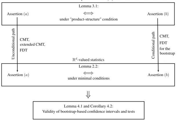
Figure 1: Summary of results; CMT stands for “continuous mapping theorem” and FDT for “functional delta method”.
5
Concluding remarks
As a picture often speaks better than words, we summarized the results obtained in this work in the diagram of Figure1. From the point of view of applications of resampling schemes starting at the stochastic process level, the diagram highlights two paths to proving the asymptotic validity of bootstrap-based confidence intervals and tests: an unconditional path starting at Assertion (a) of Lemma3.1 and a conditional path starting at Assertion (b) of Lemma 3.1.
We conclude by summarizing the main consequences and features of the results obtained in this note, some of which explicitly appear in the diagram of Figure 1:
• At the stochastic process level, it may be argued that one needs to deal with less subtle mathematical concepts to prove unconditional bootstrap consistency than to show its con-ditional version. Roughly speaking, the unconcon-ditional approach avoids the need to work with the seemingly awkward notion of “conditional law” of a non-measurable function. The fact that the joint weak convergence in Assertion (a) must be proved for all M ∈N is not an obstacle in most cases as going from the result for M = 1 to the result for all M ∈N only requires a slightly more involved proof of the weak convergence of the finite dimensional distributions, the asymptotic tightness part of the proof remaining the same.
• Focusing for instance on existing continuous mapping theoremsfor the bootstrap(Kosorok,
2008, Section 10.1.4), it appears that, for transferring Assertion (b) of Lemma 3.1 into Assertion (b) of Lemma2.2, more assumptions than just continuity of the underlying func-tional are necessary, thereby suggesting that the uncondifunc-tional formulation of bootstrap consistency might be slightly more useful. Additionally, Assertion (a) of Lemma 3.1can
be combined with the extended continuous mapping theorem (van der Vaart and Wellner,
2000, Theorem 1.11.1), a versionfor the bootstrap of which does not seem to exist.
• The equivalence between the unconditional and the conditional formulation of bootstrap consistency at the stochastic process level only holds if the additional randomness in the bootstrap replicates is independent of the data (in fact, this assumption is only needed to make Assertion (b) well-defined). Interestingly enough, such a condition does not seem to be a restriction in practice as it seems satisfied by most if not all resampling schemes. As a consequence, Lemma3.1 confirms that most bootstrap consistency results obtained under the form of Assertion (a) in the literature (see Section3for references) are not any weaker than if the (equivalent) conditional formulation in (b) were proved.
Acknowledgments
The authors would like to thank Jean-David Fermanian for fruitful discussions. This research has been supported by the Collaborative Research Center “Statistical modeling of nonlinear dynamic processes” (SFB 823) of the German Research Foundation, which is gratefully ac-knowledged.
References
R. Beran and G.R. Ducharme. Asymptotic theory for bootstrap methods in statistics. Les publication CRM, Centre de recherches math´ematiques, Universit´e de Montr´eal, Canada, 1991.
R. J. Beran, L. Le Cam, and P. W. Millar. Convergence of stochastic empirical measures. J. Multivariate Anal., 23(1):159–168, 1987.
B. Berghaus and A. B¨ucher. Goodness-of-fit tests for multivariate copula-based time series models. Econometric Theory, 33(2):292–330, 2017.
Peter J. Bickel and David A. Freedman. Some asymptotic theory for the bootstrap. Ann. Statist., 9(6):1196–1217, 11 1981.
P. Billingsley. Convergence of probability Measures. Wiley, New York, 1999. Second edition. A. B¨ucher and I. Kojadinovic. A dependent multiplier bootstrap for the sequential empirical
copula process under strong mixing. Bernoulli, 22(2), 2016a.
A. B¨ucher and I. Kojadinovic. Dependent multiplier bootstraps for non-degenerateu-statistics under mixing conditions with applications. Journal of Statistical Planning and Inference, 170:83–105, 2016b.
A. C. Davison and D. V. Hinkley. Bootstrap Methods and Their Application. Cambridge University Press, 1997. ISBN 0-521-57391-2; 0-521-57471-4.
B. Efron. Bootstrap methods: Another look at the jackknife. Ann. Statist., 7(1):1–26, 01 1979. C. Genest and J. G. Neˇslehov´a. On tests of radial symmetry for bivariate copulas. Statistical
C. Genest and B. R´emillard. Validity of the parametric bootstrap for goodness-of-fit testing in semiparametric models. Annales de l’Institut Henri Poincar´e: Probabilit´es et Statistiques, 44:1096–1127, 2008.
Evarist Gin´e and Joel Zinn. Bootstrapping general empirical measures. Ann. Probab., 18(2): 851–869, 1990.
Peter Hall. The bootstrap and Edgeworth expansion. Springer Series in Statistics. Springer-Verlag, New York, 1992.
J.L. Horowitz. The bootstrap. In J. J. Heckman and E. E. Leamer, editors, Handbook of Econometrics, volume 5, pages 3159–3228. North-Holland, Amsterdam, 2001.
Olav Kallenberg. Foundations of modern probability. Probability and its Applications (New York). Springer-Verlag, New York, second edition, 2002.
M.R. Kosorok.Introduction to empirical processes and semiparametric inference. Springer, New York, 2008.
H.R. K¨unsch. The jacknife and the bootstrap for general stationary observations. The Annals of Statistics, 17(3):1217–1241, 1989.
B. R´emillard and O. Scaillet. Testing for equality between two copulas. Journal of Multivariate Analysis, 100(3):377–386, 2009.
J. Segers. Asymptotics of empirical copula processes under nonrestrictive smoothness assump-tions. Bernoulli, 18:764–782, 2012.
X. Shao. The dependent wild bootstrap. Journal of the American Statistical Association, 105 (489):218–235, 2010.
W. Stute, W. Gonz´ales Manteiga, and M. Presedo Quindimil. Bootstrap based goodness-of-fit tests. Metrika, 40:243–256, 1993.
A.W. van der Vaart. Asymptotic statistics. Cambridge University Press, 1998.
A.W. van der Vaart and J.A. Wellner. Weak convergence and empirical processes. Springer, New York, 2000. Second edition.