Main Library Strickhofstrasse 39 CH-8057 Zurich www.zora.uzh.ch Year: 2016
Nonconvex regularization in remote sensing
Tuia, Devis ; Flamary, Rémi ; Barlaud, MichelAbstract: In this paper, we study the effect of different regularizers and their implications in high-dimensional image classification and sparse linear unmixing. Although kernelization or sparse methods are globally accepted solutions for processing data in high dimensions, we present here a study on the impact of the form of regularization used and its parameterization.We consider regularization via traditional squared (!2) and sparsity-promoting (!1) norms, as well as more unconventional non convex regularizers (!p and log sum penalty). We compare their properties and advantages on several classification and linear unmoving tasks and provide advices on the choice of the best regularizer for the problemat hand. Finally,we also provide a fully functional toolbox for the community.
DOI: https://doi.org/10.1109/TGRS.2016.2585201
Posted at the Zurich Open Repository and Archive, University of Zurich ZORA URL: https://doi.org/10.5167/uzh-126406
Journal Article Accepted Version Originally published at:
Tuia, Devis; Flamary, Rémi; Barlaud, Michel (2016). Nonconvex regularization in remote sensing. IEEE Transactions on Geoscience and Remote Sensing, 54(11):6470-6480.
Nonconvex Regularization in Remote Sensing
Devis Tuia,
Senior Member, IEEE
, Rémi Flamary, and Michel Barlaud,
Senior Member, IEEE
Abstract—In this paper, we study the effect of different regular-izers and their implications in high-dimensional image classifica-tion and sparse linear unmixing. Although kernelizaclassifica-tion or sparse methods are globally accepted solutions for processing data in high dimensions, we present here a study on the impact of the form of regularization used and its parameterization. We consider regular-ization via traditional squared(ℓ2)and sparsity-promoting(ℓ1) norms, as well as more unconventional nonconvex regularizers (ℓp and log sum penalty). We compare their properties and advantages on several classification and linear unmixing tasks and provide advices on the choice of the best regularizer for the problem at hand. Finally, we also provide a fully functional toolbox for the community.
Index Terms—Classification, hyperspectral, nonconvex, regu-larization, remote sensing, sparsity, unmixing.
I. INTRODUCTION
R
EMOTE sensing image processing [1] is a fast-moving area of science. Data acquired from satellite or airborne sensors and converted into useful information (land cover maps, target maps, mineral compositions, and biophysical parameters) have nowadays entered many applicative fields: efficient and effective methods for such conversion are therefore needed. This is particularly true for data sources such as hyperspectral and very high resolution images, whose data volume is big and structure is complex: for this reason, many traditional methods perform poorly when confronted to this type of data. The prob-lem is even more exacerbated when dealing with multisource and multimodal data, representing different views of the land being studied (different frequencies, different seasons, angles, etc.). This created the need for more advanced techniques, often based on statistical learning [2].Among such methodologies, regularized methods are cer-tainly the most successful. Using a regularizer imposes some constraints on the class of functions to be preferred during the optimization of the model and can thus be beneficial if we know what these properties are. More often, regularizers are used to favor simpler functions over very complex ones in order to avoid overfitting of the training data: in classification,
Manuscript received April 11, 2016; revised June 2, 2016; accepted June 22, 2016. This work was supported in part by the Swiss National Science Founda-tion under Grant PP00P2-150593. D. Tuia and R. Flamary contributed equally to this paper.
D. Tuia is with the University of Zurich, 8006 Zurich, Switzerland (e-mail: [email protected]).
R. Flamary is with Université Côte d’Azur, OCA, CNRS, Lagrange, 06000 Nice, France (e-mail: [email protected]).
M. Barlaud is with Université Côte d’Azur, CNRS, I3S, 06000 Nice, France. Color versions of one or more of the figures in this paper are available online at http://ieeexplore.ieee.org.
Digital Object Identifier 10.1109/TGRS.2016.2585201
the support vector machine uses this form of regularization [3], [4], while in regression, examples can be found in kernel ridge regression or Gaussian processes [5].
However, smoothness-promoting regularizers are not the only ones that can be used: depending on the properties one wants to promote, other choices are becoming more and more popular. A first success story is the use of Laplacian regulariza-tion [6]: by enforcing smoothness in the local structure of the data, one can promote the fact that points that are similar in the input space must have a similar decision function (Laplacian SVM [7], [8] and dictionary-based methods [9], [10]) or be pro-jected close after a feature extraction step (Laplacian eigenmaps [11] and manifold alignment [12]). Another popular property to be enforced, on which we will focus the rest of this paper, is sparsity [13]. Sparse models have only a part of the initial coefficients which is active (i.e., nonzero) and are thus compact. This is desirable in classification when the dimensionality of the data is very high (e.g., when adding many spatial filters [14], [15] or using convolutional neural networks [16], [17]) or in sparse coding when we need to find a relevant dictionary to express the data [18]. Even though nonsparse models can work well in terms of overall accuracy, they still store information about the training samples to be used at test time: if such information is very high dimensional and the number of training samples is important, the memory requirements, the model complexity, and—as a consequence—the execution time are strongly affected. Therefore, when processing next-generation large data using models generating millions of features [19], [20], sparsity is very much needed to make models portable while remaining accurate. For this reason, sparsity has been extensively used in the following: 1) spectral unmixing [21], where a large variety of algorithms is deployed to select end-members as a small fraction of the existing data [18], [22], [23]; 2) image classification, where sparsity is promoted to have portable models either at the level of the samples used in reconstruction-based methods [24], [25] or in feature selection schemes [15], [26], [27]; and 3) and more focused applications such as 3-D reconstruction from SAR [28], phase estimation [29], or pansharpening [30].
A popular approach to recover sparse features is to solve a convex optimization problem involving theℓ1norm (or Lasso)
regularization [31]–[33]. Proximal splitting methods have been shown to be highly effective in solving sparsity-constrained problems [34]–[36]. The Lasso formulation based on the penalty on theℓ1norm of the model has been shown to be an
efficient shrinkage and sparse model selection method in re-gression [37]–[39]. However, the Lasso regularizer is known to promote biased estimators, leading to suboptimal classification performances when strong sparsity is promoted [40], [41]. A way out of this dilemma between sparsity and performance is to retrain a classifier, this time nonsparse, after the feature 0196-2892 © 2016 IEEE. Personal use is permitted, but republication/redistribution requires IEEE permission.
selection has been performed with Lasso [15]. Such scheme works but at the price of training a second model, thus leading to extra computational effort and to the risk of suboptimal solu-tions, since we are training a model with the features that were considered optimal by another. In unmixing, synthetic exam-ples also show that theℓ1regularization is not the one leading
to the best abundance estimation [42].
In recent years, there has been a trend in the study of unbiased sparse regularizers. These regularizers, typically theℓ0,ℓq, and
log sum penalty (LSP) [40], can solve the dilemma between sparsity and performance but are nonconvex and therefore cannot be solved by known off-the-shelf convex optimization tools. Therefore, such regularizers have until now received little attention in the remote sensing community. A handful of papers usingℓqnorm is found in the field of spectral unmixing
[42]–[44], where authors consider nonnegative matrix factor-ization solutions; in the modeling of electromagnetic induction responses, where the model parameters were estimated by regu-larized least squares estimation [45]; in feature extraction using deconvolutional networks [46]; and in structured prediction, where authors use a nonconvex sparse classifier to provide posterior probabilities to be used in a graph cut model [47]. In all of these studies, the nonconvex regularizer outperformed the
ℓ1while still providing sparse solutions.
In this paper, we give a critical explanation and theoretical motivations for the success of regularized classification, with a focus on nonconvex methods. By comparing it with other tradi-tional regularizers (ridgeℓ2and Lassoℓ1), we advocate the use
of nonconvex regularization in remote sensing image process-ing tasks: nonconvex optimization marries the advantages of accuracy and sparsity in a single model, without the need of unbiasing in two steps or reducing the level of sparsity to in-crease performance. We also provide a freely available toolbox for the interested readers that would like to enter this growing field of investigation.
The remainder of this paper is organized as follows. In Section II, we present a general framework for regularized remote sensing image processing and discuss different forms of convex and nonconvex regularization. We will also present the optimization algorithm proposed. Then, in Section III, we apply the proposed nonconvex regularizers to the problem of multi-and hyperspectral image classification multi-and therefore present the specific data term for classification and study it in synthetic and real examples. In Section IV, we apply our proposed framework to the problem of linear unmixing, present the specific data term for unmixing, and study the behavior of the different regularizers in simulated examples involving true spectra from the USGS library. Section V concludes this paper.
II. OPTIMIZATION ANDNONCONVEXREGULARIZATION In this section, we give an intuitive explanation of regularized models. We first introduce the general problem of regulariza-tion and then explore convex and nonconvex regularizaregulariza-tion schemes, with a focus on sparsity-inducing regularizers. Fi-nally, we present the optimization algorithms to solve non-convex regularization, with accent put on proximal splitting methods such as general iterative shrinkage and thresholding (GIST) [48].
TABLE I
DEFINITION OF THEREGULARIZATIONTERMSCONSIDERED
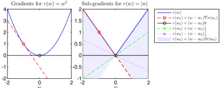
Fig. 1. Illustration of the regularization termsg(·). Note that bothℓ2andℓ1 regularizations are convex and that LSP andℓpwithp= 1/2are concave on their positive orthant.
A. Optimization Problem
Regularized models address the following problem:
min
w∈Rd
L(w) +λR(w) (1) whereL(·)is a smooth function (Lipschitz gradient),λ>0is a
regularization parameter, andR(·)is a regularization function. This kind of problem is extremely common in data mining, denoising, and parameter estimation.
L(·) is often an empirical loss that measures the discrep-ancy between a modelw and a data set containing real-life observations.
The regularization term R(·) is added to the optimization problem in order to promote a simple model, which has been shown to lead to a better estimation [49]. All of the regulariza-tion terms discussed in this paper are of the form
R(w) =!
k
g(|wk|) (2)
wheregis a monotonically increasing function. This means that the complexity of the modelwcan be expressed as a sum of the complexity of each featurekin the model.
The specific form of the regularizer will change the as-sumptions made on the model. In the following, we discuss several classes of regularizers of increasing complexity: differ-entiable, nondifferentiable (i.e., sparsity inducing), and, finally, both nondifferentiable and nonconvex. A summary of all of the regularization terms investigated in this paper is given in Table I, along with an illustration of the regularization as a function of the value of the coefficientwk(Fig. 1).
B. Nonsparse Regularization
One of the most common regularizers is the squareℓ2norm
of modelw, i.e.,R(w) ="w"2(g(·) = (·)2)
. This regulariza-tion will penalize large values in the vectorwbut is isotropic, i.e., it will not promote a given direction for the vector w. This regularization term is also known asℓ2, quadratic, or ridge
regularization and is commonly used in linear regression and classification. For instance, logistic regression is often regular-ized with a quadratic term. Also, note that the support vector machine is regularized using the ℓ2 norm in the reproducing
kernel Hilbert space of the formR(w) =w⊤Kw[50]. C. Sparsity-Promoting Regularization
In some cases, not all of the features or observations are of interest for the model. In order to get a better estimation, one wants the vectorwto be sparse, i.e., to have several components exactly 0. For linear prediction, sparsity in the modelwimplies that not all features are used for the prediction.1This means that
the features showing a nonzero value inwkare then “selected.”
Similarly, when estimating a mixture, one can suppose that only few materials are present, which again implies sparsity of the abundance coefficients.
In order to promote sparsity inw, one needs to use a regu-larization term that increases when the number of active com-ponents grows. The obvious choice is to use theℓ0pseudonorm
that returns directly the number of nonzero coefficients inw. Nevertheless, theℓ0 term is nonconvex and nondifferentiable
and cannot be optimized exactly unless all of the possible sub-sets are tested. Despite recent works aiming at solving directly this problem via discrete optimization [51], this approach is still computationally impossible even for medium-sized problems. Greedy optimization methods have been proposed to solve this kind of optimization problem and have led to efficient algorithms such as orthogonal matching pursuit (OMP) [52] or orthogonal least square (OLS) [53]. However, one of the most common approaches to promote sparsity without recurring to theℓ0regularizer is to use theℓ1norm instead. This approach,
also known as the Lasso in linear regression, has been widely used in compressive sensing in order to estimate with precision a few components in a large sparse vector.
Now, we discuss the intuition why using a regularization term such asℓ1promotes sparsity. The reason behind the sparsity of
theℓ1norm lies in the nondifferentiability at 0 shown in Fig. 1
(dashed blue line). For the sake of readability, we will suppose here thatR(·)is convex, but the intuition is the same, and the results can be generalized to the nonconvex functions presented in the next section. For a more illustrative example, we use a 1-D comparison between theℓ2andℓ1regularizers (Fig. 2).
• When both the data and regularization term are differen-tiable, a stationary pointw⋆has the following property:
∇L(w⋆) +λ∇R(w⋆
) =0. (3)
In other words, the gradients of both functions have to cancel themselves exactly. This is true for theℓ2
regular-izer everywhere, but also for theℓ1, with the exception of
wk= 0. If we consider theℓ2regularizer as an example
(left plot in Fig. 2), we see that each point has a specific gradient, corresponding to the tangent to each point (e.g., the red dashed line). The stationary point is reached in this case forwk = 0, as given by the black line at the left plot
of Fig. 2.
1Note that zero coefficients might happen also in theℓ
2 solution, but the regularizer itself does not promote their appearance.
Fig. 2. Illustration of gradients and subgradients on differentiableℓ2(left) and nondifferentiableℓ1(right) functions.
• When the second term in (3) is not differentiable (as in theℓ1case at 0 presented at the right plot of Fig. 2), the
gradient is not unique anymore, and one has to use the subgradients and subdifferentials. For a convex function R(·), a subgradient atwtis a vectorxsuch thatR(w)≥
x⊤(w−wt) +R(wt), i.e., it is the slope of a
lin-ear function that remains below the function. In 1-D, a subgradient defines a line touching the function at the nondifferentiable point (in the case of Fig. 2, at 0) but stays below the function everywhere else, e.g., the black and green dotted-dash lines in Fig. 2 (right). The subdifferential∂R(wt)is the set of all of the subgradients
that respect the aforementioned minoration relation. The subdifferential is illustrated in Fig. 2 by the area in light blue, which contains all possible solutions.
Now the optimality constraints cannot rely on equality since the subgradient is not unique, which leads to the following optimality condition:
0∈ ∇L(w⋆) +λ∂R(w⋆). (4) This is very interesting in our case because this condition is much easier to satisfy than (3). Indeed, we just need to have a single subgradient in the whole subdifferential
∂R(·)that can cancel the gradient∇L(·). In other words,
only one of the possible straight lines in the blue area is needed to cancel the gradient, thus making the chances for a null coefficient much higher. For instance, when using theℓ1regularization, the subdifferential of variablewkin
0 is the set[−λ,λ]. Whenλbecomes large enough, it is
larger than all of the components of the gradient∇L(·), and the only solution verifying the conditions is the null vector0.
Theℓ1regularization has been largely studied. Because it is
convex, it means that it avoids the problem of local minima, and many efficient optimization procedures exist to solve it (e.g., LARS [54] and forward backward splitting [55]). However, the sparsity of the solution using ℓ1 regularization often comes
with a cost in terms of generalization. While theoretical studies show that, under some constraint, the ℓ1 can recover the true
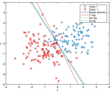
relevant variables and their sign, the solution obtained will be biased toward0[56]. Fig. 3 illustrates the bias in a two-class toy data set: theℓ1 decision function (red line) is biased with
respect to the Bayes decision function (blue line). In this case, the bias corresponds to a rotation of the separating hyperplane. In practice, one can deal with this bias by estimating again the
Fig. 3. Example of a two-class toy example with 2 discriminant features and 18 noisy features. The regularization parameter of each method has been chosen as the minimal value that leads to the correct sparsity with only two features selected.
model on the selected subset of variables using an isotropic norm (e.g.,ℓ2) [15], but this requires us to solve again an optimization
problem. The approach that we propose in this paper is to use a nonconvex regularization term that will still promote sparsity while minimizing the aforementioned bias. To this end, we present nonconvex regularization in the next section.
D. Nonconvex Regularization
In order to promote more sparsity while reducing the bias, several works have looked at nonconvex yet continuous regu-larization. Such regularizers have been proposed, for instance, in statistical estimation [57], compressed sensing [40], or ma-chine learning [41]. Popular examples are the smoothly clipped absolute deviation [57], the minimax concave penalty [58], and the LSP [40] considered in the following (see [48] for more examples). In the following, we will investigate two of them in more detail:ℓp pseudonorm withp= 1/2and LSP, both also
displayed in Fig. 1.
All of the aforementioned nonconvex regularizations share some particular characteristics that make them of interest in our case. First (and as the ℓ0 pseudonorm and ℓ1 norm), they all
have a nondifferentiability in0, which—as we have seen in the previous section—promotes sparsity. Second, they are all con-cave in their positive orthant, which limits the bias because their gradient will decrease for large values ofwk limiting the
shrinkage (as compared to the ℓ1 norm, whose gradient for
wk '= 0 is constant). Intuitively, this means that, with a
non-convex regularization, it will become more difficult for large coefficients to be shrunk toward 0 because their gradient is small. On the contrary, the ℓ1 norm will treat all coefficients
equally and apply the same attraction to the stationary point to all of them. The decision functions for the LSP andℓpnorms are
shown in Fig. 3 and are much closer to the actual (true) Bayes decision function.
E. Optimization Algorithms
Owing to the differentiability of theL(·)term, the optimiza-tion problem can be solved using proximal splitting methods [55]. The convergence of those algorithms to a global minimum is well studied in the convex case. For nonconvex regulariza-tion, recent works have proved that proximal methods can be used with nonconvex regularizers when a simple closed-form solution of the proximity operator for the regularization can be computed [48]. Authors in [59] have studied the convergence to a local stationary point of proximal methods with nonconvex regularization for several loss functions.
In this paper, we used the GIST algorithm proposed in [48]. This approach is a first-order method that consists in iteratively linearizingL(·)in order to solve very simple proximal opera-tors at each iteration. At each iterationt+ 1, one computes the model updatewt+1 by solving min w ∇L(wt)⊤(w−wt) +λR(w) +µ 2"w−w t"2 2. (5)
When µ is a Lipschitz constant of L(·), the aforementioned cost function is a majorization ofL(·) +λR(·)which ensures
a decrease of the objective function at each iteration. Problem (5) can be reformulated as a proximity operator
proxλR(v) = arg minw λR(w) +
µ
2"w−v
t"2 2 (6)
wherevt=wt−(1/µ)∇L(wt)can be seen as a gradient step
w.r.t. L(·) followed by a proximal operator at each iteration. Note that the efficiency of a proximal algorithm depends on the existence of a simple closed-form solution for solving the proximity operator in (6). Luckily, numerous operators exist in the convex case (detailed list in [55]), and some nonconvex proximal operators can be computed on the regularization used in our work (see [48, Appendix 1] for LSP and [60, eq. 11] for
ℓp withp= 1/2). Note that efficient methods which estimate
the Hessian matrix [61], [62] exist, as well as a wide range of methods based on DC programming, which have shown to work very well in practice [62], [63] and can handle the general casep∈(0,1]for theℓppseudonorm (see [64] for an
implementation).
Finally, when one wants to perform variable selection using theℓ0 pseudonorm as regularization, the exact solution of the
combinatorial problem is not always necessary. As mentioned previously, greedy optimization methods have been proposed to solve these optimization problems and have led to efficient algorithms as OMP [52] or OLS [53]. In this paper, we will not consider these methods in detail, but they have been shown to perform well on least square minimization problems.
III. CLASSIFICATIONWITHFEATURESELECTION In this section, we tackle the problem of sparse classification. Through a toy example and a series of real-data experiments, we will study the interest of nonconvex regularization.
A. Model
The model that we will consider in the experiments is a simple linear classifier of the form f(x) =w⊤x+b, where w∈Rdis the normal vector to the separating hyperplane andb
is a bias term. In the binary case(yi∈[−1; 1]), the estimation
is performed by solving the regularized optimization problem
min w,b 1 n n ! i=1 L(yi, f(xi)) +R(w) (7)
where R(w) is one of the regularizers in Table I and L(yi, f(xi)) is a classification loss that measures the
dis-crepancy between the predictionf(xi)and the true label yi.
Hereafter, we will use the squared hinge loss L(yi, f(xi)) = max(0,1−yif(xi))
2
.
When dealing with multiclass problems, we use a one-against-all procedure, i.e., we learn one linear functionfj(·)
per classjand then predict the final class for a given observed pixel x as the solution of arg minjfj(x). In practice, this
leads to an optimization problem similar to (7), where we need to estimate a matrix W, containing the coefficients per each class. The number of coefficients to be estimated is therefore the size d of the input space multiplied by the number of classesCplus one bias coefficient per class.
B. Toy Example
First, we consider in detail the toy example in Fig. 3: the data considered are 20-dimensional, where the first two dimensions are discriminative (they correspond to those plotted in Fig. 3), while the others are not (they are generated as Gaussian noise). The correct solution is therefore to assign nonzero coefficients to the two discriminative features and wk = 0 for all of the
others.
Fig. 3 shows the classifiers estimated for the smallest value of the regularization termλ, which leads to the correct sparsity
level (two features selected). This ensures that we have selected the proper components while minimizing the bias for all meth-ods. This also illustrates that theℓ1classifier has a stronger bias
(i.e., provides a decision function further away from the optimal Bayes classifier) than the classifiers regularized by nonconvex functions.
Let us now focus on the effect of the regularization term and of its strength, defined by the regularization parameterλ
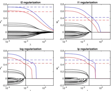
in (7). Fig. 4 illustrates a regularization path, i.e., all of the solutions obtained by increasing the regularization parameter
λ.2Each line corresponds to one input variable, and those with
the largest coefficients (and in color) are the discriminative ones. Considering theℓ2regularization (top left panel in Fig. 4),
no sparsity is achieved, and even if the two correct features have the largest coefficients, the solution is not compact. The
ℓ1 solution (top right panel) shows a correct sparse solution
forλ= 10−1
(vertical black line, where all of the coefficients but two are 0), but the smallest coefficient is biased (it is smaller than expected by the Bayes classifier, represented by the horizontal dashed lines). The two nonconvex regularizers (bottom line of Fig. 4) show the correct features selected but
2A “regularization path” for theℓ
1is generally computed using homotopy algorithms [65]. However, experiments show that the computational complexity of the completeℓ1 path remains high for high-dimensional data. Therefore, in our experiments, we used an approximate path (i.e., a discrete sampling of λvalues along the path).
Fig. 4. Regularization paths for the toy example in Fig. 3. Each line corre-sponds to the coefficients wk attributed to each feature along the different values ofλ. The best fit is met for each regularizer at the black vertical line, where all coefficients but two are 0. The unbiased Bayes classifier coefficients (the correct coefficients) are represented by the horizontal dashed lines. a smaller bias: the coefficient retrieved is closer to the optimal ones of the Bayes classifier. Moreover, the nonzero coefficients stay close to the correct values for a wider set of regularization parameters and then drop directly to zero: this means that the nonconvex model either does not have enough features to train or has little features with the right coefficients, contrary to the
ℓ1that can retrieve a sparse solution with wrong coefficients, as
seen in the part to the right of the vertical black line of theℓ1
regularization path. C. Remote Sensing Images
Data: The real data sets considered are three very high resolution remote sensing images.
1) Thetford mines. The first data set is acquired over the Thetford mines site in Québec, Canada, and contains two data sources: a VHR color image (three channels, red-green-blue) at 20-cm resolution and a long wave infrared (LWIR, 84 channels) hyperspectral image at approximately 1-m resolution.3 The LWIR images are
downsampled by a factor 5 to match the resolution of the RGB data, leading to a(4386×3769×87)datacube. A 7-classes ground truth is available. The RGB composite, band 1 of te LWIR data and train/test ground truths are provided in Fig. 5.
2) Houston. The second image is a CASI image acquired over Houston with 144 spectral bands at 2.5-m resolution. A field survey is also available (14703 labeled pixels, divided in 14 land use classes). A LiDAR DSM was also available and was used as an additional feature.4The CASI
3The data were proposed as the Data Fusion Contest 2014 [66] and are available on the IADF TC website for download http://www.grss-ieee.org/ community/technical-committees/data-fusion/.
4The data were proposed as the Data Fusion Contest 2013 [67] and are available on the IADF TC website for download http://www.grss-ieee.org/ community/technical-committees/data-fusion/.
Fig. 5. Thetford mines 2014data set used in the classification experiments, along with its labels. (a) RGB. (b) LWIR band 1. (c) Ground truth training. (d) Ground truth test.
Fig. 6. Houstondata set used in the classification experiments. (Top) True color representation of the hyperspectral image (144 bands). (Middle) Detrended LiDAR DSM. (Bottom) Labeled samples (all of the available ones, in 15 classes).
image was corrected with histogram matching for a large shadowed part at the right side (as in [27]), and the DSM was detrended by a 3-m trend at the left-right direction. Image, DSM, and ground truth are illustrated in Fig. 6. 3) Zurich summer. The third data set is a series of 20
QuickBird tiles issued from a single image acquired over the city of Zurich, Switzerland, in August 2002.5The data
have been pansharpened at 0.6-m spatial resolution, and 5The data set is freely available at https://sites.google.com/site/ michelevolpiresearch/data/zurich-dataset/.
Fig. 7. Example on tile #3 of the superpixels extracted by the Felzenszwalb algorithm [69].
a dense ground truth is provided for each image. Eight classes are depicted: buildings, roads, railway, water, swimming pools, trees, meadows, and bare soil. More information on the data can be found in [68]. To reduce computational complexity, we extracted a set of superpix-els using the Felzenszwalb algorithm [69], which reduced the number of samples from∼106
pixels per image to a few thousands. An example of the superpixels extracted on image tile #3 is given in Fig. 7.
Setup: For all data sets, contextual features were added to the spectral bands in order to improve the geometric quality of classification [14]: morphological and texture filters were added, following the list in [15]. Each image was processed to extract the most effective filters for its processing.
• For theThetford minesdata set, the filters were extracted from the RGB image and from a normalized ratio be-tween the red band and the average of the LWIR bands (following the strategy of the winners of the 2014 Data Fusion Contest [66]), which approaches a vegetation in-dex. Given the extremely high resolution of the data set, the filters were computed with the size range{7, . . .23}, leading to 100 spatial features.
• For theHoustoncase, the filters were calculated on the three first principal component projections extracted from the hyperspectral image and on the DSM. Given the smaller resolution of this data set, the convolution sizes of the local filters are in the range{3, . . . ,15}pixels. This leads to 240 spatial features.
• For theZurich summerdata set, spatial filters were com-puted directly on the four spectral bands, plus the NDVI and the NDWI indices. Then, average, minimum, maxi-mum, and standard deviation values per superpixel were extracted as feature values. Since the spatial resolution is comparable to the one of theHoustondata sets, the same sizes of convolution filters are used, leading to a total of 360 spatial features.
The joint spatial–spectral input space is obtained by stacking the original images to the spatial filters above. It is therefore of dimension 188 in theThetford minesdata, 384 in theHouston data, and 366 in theZurich summercase.
Regarding the classifier, we considered the linear classifier of (7) with a squared hinge loss.
• In the Thetford minescase, we use 5000 labeled pixels per class. Given the spatial resolution of the image and
Fig. 8. Five test images of the Zurich summer data set (from left to right, tiles #16 to #20), along with their ground truth.
Fig. 9. Performance (kappa) versus compactness (number of coefficients wj,k>0) for the different regularizers in theThetford mines, Houston, and
Zurich summerdata sets.
the 568242 labeled points available in the training ground truth, this only represents approximately 5% of the la-beled pixels in the training image. For the test, we use the entire test ground truth, which is spatially disconnected to the training one (except for the class “soil”; see Fig. 5) and carries 1.5 million labeled pixels.
• In the Houstoncase, we also proceed with pixel classi-fication. All of the models are trained with 60 labeled pixels per class, randomly selected, from the available training data. We report performances on the entire test set provided in the Data Fusion Contest 2013, which is spatially disconnected from the training set (Fig. 6). • For theZurich summerdata, we deal with superpixels and
20 separate images. We used images #1–15 to train the classifier and then tested on the five remaining images (Fig. 8). Given the complexity of the task (not all of the images have all of the classes and the urban fabrics depicted vary from scene to scene), we used 90% of the available superpixels in the 15 training images, which re-sulted in 30649 superpixels. All of the labeled superpixels in the test images (8960 superpixels) are used as test set. Regarding the regularizers, we compare the four regularizers of Table I (ℓ1, ℓ2, LSP, andℓpwithp= 1/2) and study the joint
behavior of accuracy and sparsity along a regularization path, i.e., for different values ofλ={1e−5, . . . ,1e−1}
, with 18 steps. For each step, the experiment was repeated ten times with different train/test sets (each run with the same training samples for all regularizers), and the average kappa and number of active
coefficients are reported in Fig. 9. Also, note that we report the total number of coefficients in the multiclass case|wj,k|, which
is equal to the number of features multiplied by the number of classes, plus one additional feature per class (bias term). In total, the model estimates 1504 coefficients in the case of the Thetford minesdata, while for theHoustonandZurich summer cases, it deals with 5775 and 3294 coefficients, respectively.
Results: The results are reported in Fig. 9, comparing the regularization paths for the four regularizers and the three data sets presented previously. The graphs can be read as a ROC curve: the most desirable situation would be a classifier with both accuracy and little active features, i.e., a score close to the top-left corner. Theℓ2model shows no variation on the sparsity
axis (all of the coefficients are active) and very little variability on the accuracy one: it is therefore represented by a single green dot. It is remarkably accurate but is the less compact model since it has all of the coefficients active. Employing the ℓ1
regularizer (red line), as it is mainly done in the literature of sparse classification, achieves a sharp decrease in the number of active coefficients but at the price of a steep decrease in per-formances of the classifier. When using 100 active coefficients, the ℓ1 model suffers from a 20% drop in performance, and a
trend is observed in all of the experiments.
Using the nonconvex regularizers provides the best of both worlds: theℓpregularizer (black line with “!” markers) in
par-ticular and also the LSP regularizer (blue line with “×” markers) achieve improvements of about 15%–20% with respect to the
observed: the nonconvex regularizers are less biased than the
ℓ1norm in classification and achieve competitive performances
with respect to the (nonsparse)ℓ2model with a fraction of the
features (around 1%–2%). Note that the models of all experi-ments were initialized with the0vector. This is sensible for the nonconvex problem since all of the regularizations discussed in this paper (evenℓ2) tend to shrink the model toward this point.
By initializing at 0for nonconvex regularization, we simply promote a local solution not too far from this neutral point. The initialization can be seen as an additional regularization. Moreover, the experiments show that the nonconvexity leads to state-of-the-art performance.
IV. SPARSELINEARUNMIXING
In this section, we express the sparse linear unmixing prob-lem in the same optimization framework as (7). We discuss the advantage of using nonconvex optimization. The performances of theℓ2,ℓ1, nonconvexℓp, and LSP regularization terms are
then compared on a simulated example using real reflectance spectra (as in [18]).
A. Model
Sparse linear unmixing can be expressed as the following optimization problem: min α≥0 1 2"y−Dα" 2 2+λR(α) (8)
where y is a noisy spectrum observed and D is a matrix containing a dictionary of spectra (typically a spectral library). This formulation adds a positivity constraint to the vector α w.r.t. problem (7). In practice, (8) can be reformulated as the following unconstrained optimization problem:
min α 1 2"y−Dα" 2 2+λR(α) +ıα≥0 (9)
whereıα≥0 is the indicator function that has a value of +∞
when one of the components of α is <0 and a value of 0 when it is in the positive orthant. By supposing that ıα≥0
is equivalent to λıα≥0,∀λ>0, we can gather the last two
terms into R˜(α) =R(α) +ıα≥0, thus leading to a problem
similar to (7). All of the optimization procedures discussed previously can therefore be used for this reformulation as long as the proximal operator w.r.t.R˜(·)can be computed efficiently. The proximal operator for all of the regularization terms in Table I with additional positivity constraints can be obtained by an orthogonal projection on the positive orthant followed by the proximal ofR
proxλR+ıα≥0(v) =proxλR(max(v,0)) (10) wheremax(v,0)is taken componentwise. This shows that we can use the same algorithm as in the classification experiments of Section III since we have an efficient proximal operator.
We know that in practice the true components of alpha are sparse (only a few component in each spectrum). To promote this sparsity we use a nondifferentiable regularization term R(α) in equation (8). Therefore, in the following, we investigate the use of nonconvex regularization for linear unmixing. We focus on problem (8), but a large part of the unmixing literature
works with an additional constraint of sum to 1 for the α coefficients. This additional prior can sometimes reflect a phys-ical measure and adds some information to the optimization problem. In our framework, this constraint can make the direct computation of the proximal operator nontrivial. In this case, it is more interesting to use multiple splitting instead of one and to use other algorithms such as generalized FBS [70] or ADMM, which has already been used for remote sensing applications [71].
B. Numerical Experiments
In the unmixing application, we consider an example sim-ulated using the USGS spectral library6: from the library, we
extract 23 spectra corresponding to different materials (by keep-ing spectra with less than 15◦angular distance to each other). Using these 23 base spectra, we simulate mixed pixels by cre-ating random linear combinations ofnact≤23endmembers.
The random weight of the active components is obtained using a uniform random generation in [0, 1] (leading to weights that do not sum to 1). We then add to the resulting signatures some Gaussian noisen∼N(0,σ2)
. For each numerical experiment, we solve the unmixing problem by least squares with the four regularizers of Table I: ℓ2, ℓ1, ℓp, and LSP. An additional
approach that consists in performing a hard thresholding on the positive least square solution (so the ℓ2) has also been
investigated (named “LS+threshold” hereafter). As for the previous example on classification, we calculate the unmixing performance on a regularization path, i.e., a series of values of the regularization parameterλin (8), withλ= [10−5
, . . . ,103
]. We assess the success of the unmixing by the model error
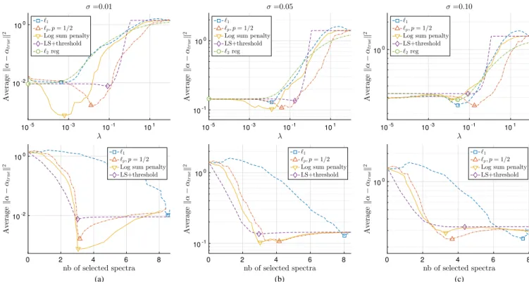
"α−αtrue"2. We repeat the simulation 50 times to account for different combinations of the original elements of the dictio-nary: all results reported are averages over those 50 simulations. First, we compare the different regularization schemes for different noise levels (Fig. 10). We setnact= 3and report the
model error along the regularization path (varyingλ) at the top
row of Fig. 10. At the bottom row, we report the model error as a function of the number of selected components, again along the same regularization path. We observe that the nonconvex strate-gies achieve the lowest errors (triangle-shaped markers) on low and medium noise levels but also that ℓp seems to be more
robust to noise. The ℓ1 norm also achieves good results,
par-ticularly in high-noise situations. Regarding the error achieved per level of sparsity (represented at the bottom row of Fig. 10), we observe that the nonconvex regularizers achieve far better reconstruction errors, particularly around the right number of active coefficients (herenact= 3). On average, the best results
are obtained by the LSP andℓpregularization. Note that theℓ1
regularizer needs a larger number of active components in order to achieve good model reconstruction (on the order of 9 when the actual number of coefficients is 3). The LS+threshold approach seems to work well for component selection but leads to an important decrease in accuracy of the model.
In order to evaluate the ability of a method to estimate a good model and select the good active components at the same time, we run simulations with a fixed noise levelσ= 0.05but
Fig. 10. Linear unmixing results on the simulated hyperspectral data set. Each column represents a different noise level. (a) σ= 0.01. (b) σ= 0.05. (c)σ= 0.10. Model error!α−αtrue!2is plotted as a function either of the regularization parameterλ(top row) or of the number of active coefficients of the final solution (bottom row). The marker shows the best performances of each regularization strategy.
Fig. 11. Linear unmixing results on the simulated hyperspectral data set for increasing number of active spectra in the mixture: (a) model error for the best solution with the number of selected spectra closest tonactand (b) number of selected spectra for the model with the lowest error.
for a varying number of true active components nact, from
1 to 23. In this configuration, we first find for all regularizations the smallest λ that leads to the correct number of selected
component nsel=nact. The average model error as a
func-tion of nact is reported in Fig. 11(a). We can see that the
nonconvex regularization leads to better performances when the correct number of spectra is selected (compared to ℓ1
and LS+threshold). In Fig. 11(b), we report the number of selected components as a function of the true number of active components when the model error is minimal. We observe that nonconvex regularization manages to both select the correct components and estimate a good model when a small number of components are active (nact≤10) but also that it fails
(as ℓ1 does) for large numbers of active components. This
result illustrates the fact that nonconvex regularization is more aggressive in terms of sparsity and obviously performs best when sparsity is truly needed.
V. CONCLUSION
In this paper, we have presented a general framework for nonconvex regularization in remote sensing image processing. We have discussed different ways to promote sparsity and avoid the bias when sparsity is required via the use of nonconvex reg-ularizers. We have applied the proposed regularization schemes to problems of image classification and linear unmixing: in all scenarios, we have showed that nonconvex regularization leads to the best performances when accounting for both sparsity and quality of the final product. Nonconvex regularizers promote compact solutions but without the bias (and the decrease in performance) related to nondifferentiable convex norms such as the popularℓ1norm.
Nonconvex regularization is a flexible and general frame-work that can be applied to every regularized processing scheme: keeping this in mind, we have also provided a toolbox to the community to apply nonconvex regularization to a wider number of problems. The toolbox can be accessed in Github (see the Appendix for a description of the toolbox).
APPENDIX OPTIMIZATIONTOOLBOX
To promote the use of nonconvex regularization in the remote sensing community, we provide the reader with a simple to use MATLAB/Octave generic optimization toolbox. The code provides a generic solver (complete rewriting of GIST) for problem (7) that is able to handle a number of regularization terms (at least all of the terms in Table I) and any differentiable data fitting termL. We provide several functions for performing multiclass classification tasks such as SVM, logistic regression,
and calibrated hinge loss. For linear unmixing, we provide the least squares loss, but extension to other more robust data fitting terms can be performed easily. For instance, performing unmixing with the Huber loss [72] would require the change of two lines in function “gist_least.m,” i.e., the compu-tation of the Huber loss and its gradient. The toolbox is avail-able at https://github.com/rflamary/nonconvex-optimization. It is freely available as a community project, and we welcome contributions.
ACKNOWLEDGMENT
The authors would like to thank the IEEE GRSS Image Analysis and Data Fusion Technical Committee (IADFTC) for organizing and making available the data of the Data Fusion Contests 2013 and 2104. For the contest 2014, they also ac-knowledge Telops Inc. (Québec, Canada) for acquiring and pro-viding the Thetford mines data, the Centre de Recherche Public Gabriel Lippmann and Dr. M. Schlerf for their contribution on the Hyper-Cam LWIR sensor, Dr. M. De Martino (University of Genoa, Genova, Italy) for providing the ground truth and Dr. M. Shimoni (Royal Military Academy, Belgium) for orga-nizing the contest. For the 2013 contest, they also acknowledge the Hyperspectral Image Analysis Group and the NSF Funded Center for Airborne Laser Mapping (NCALM) at the University of Houston, Houston, TX, USA, for providing the Houston data. Finally, the authors acknowledge Dr. Volpi and Dr. Longbotham for making the Zurich summer data available, and Dr. Iordache and Dr. Bioucas-Dias for sharing the USGS library used in the unmixing experiment.
REFERENCES
[1] G. Camps-Valls, D. Tuia, L. Gómez-Chova, S. Jimenez, and J. Malo,
Remote Sensing Image Processing, ser. Synthesis Lectures on Image, Video, and Multimedia Processing. Vermont, Vic., Australia: Morgan and Claypool, 2011.
[2] G. Camps-Valls, D. Tuia, L. Bruzzone, and J. Benediktsson, “Advances in hyperspectral image classification: Earth monitoring with statistical learning methods,”IEEE Signal Process. Mag., vol. 31, no. 1, pp. 45–54, Jan. 2014.
[3] G. Camps-Valls and L. Bruzzone, “Kernel-based methods for hyperspec-tral image classification,” IEEE Trans. Geosci. Remote Sens., vol. 43, no. 6, pp. 1351–1362, Jun. 2005.
[4] G. Mountrakis, J. Ima, and C. Ogole, “Support vector machines in remote sensing: A review,”ISPRS J. Photogramm. Remote Sens., vol. 66, no. 3, pp. 247–259, 2011.
[5] J. Verrelstet al., “Machine learning regression algorithms for biophysical parameter retrieval: Opportunities for Sentinel-2 and -3,”Remote Sens. Environ., vol. 118, pp. 127–139, 2012.
[6] M. Belkin, I. Matveeva, and P. Niyogi, “On manifold regularization,” in
Proc. 10th Int. Workshop AISTAT, Bonn, Germany, 2005, pp. 17–24. [7] L. Gómez-Chova, G. Camps-Valls, J. Muñoz-Marí, and J. Calpe,
“Semi-supervised image classification with Laplacian support vector machines,”
IEEE Geosci. Remote Sens. Lett., vol. 5, no. 4, pp. 336–340, 2008. [8] M. A. Bencherif, J. Bazi, A. Guessoum, N. Alajlan, F. Melgani, and
H. Alhichri, “Fusion of extreme learning machine and graph-based op-timization methods for active classification of remote sensing images,”
IEEE Geosci. Remote Sens. Lett., vol. 12, no. 3, pp. 527–531, Mar. 2015. [9] W. Zhangyang, N. Nasrabadi, and T. S. Huang, “Semisupervised hy-perspectral classification using task-driven dictionary learning with Laplacian regularization,” IEEE Trans. Geosci. Remote Sens., vol. 53, no. 3, pp. 1161–1173, Mar. 2015.
[10] X. Sun, N. Nasrabadi, and T. Tran, “Task-driven dictionary learning for hyperspectral image classification with structured sparsity constraints,”
IEEE Trans. Geosci. Remote Sens., vol. 53, no. 8, pp. 4457–4471, Aug. 2015.
[11] S. T. Tu, J. Y. Chen, W. Yang, and H. Sun, “Laplacian eigenmaps-based polarimetric dimensionality reduction for SAR image classifica-tion,”IEEE Trans. Geosci. Remote Sens., vol. 50, no. 1, pp. 170–179, Jan. 2012.
[12] D. Tuia, M. Volpi, M. Trolliet, and G. Camps-Valls, “Semisupervised manifold alignment of multimodal remote sensing images,”IEEE Trans. Geosci. Remote Sens., vol. 52, no. 12, pp. 7708–7720, Dec. 2014. [13] D. L. Donoho, “Compressed sensing,”IEEE Trans. Inf. Theory, vol. 52,
no. 4, pp. 1289–1306, Apr. 2006.
[14] M. Fauvel, Y. Tarabalka, J. A. Benediktsson, J. Chanussot, and J. C. Tilton, “Advances in spectral–spatial classification of hyperspectral images,”Proc. IEEE, vol. 101, no. 3, pp. 652–675, Mar. 2013.
[15] D. Tuia, M. Volpi, M. Dalla Mura, A. Rakotomamonjy, and R. Flamary, “Automatic feature learning for spatio-spectral image classification with sparse SVM,” IEEE Trans. Geosci. Remote Sens., vol. 52, no. 10, pp. 6062–6074, Oct. 2014.
[16] C. Romero, A. und Gatta, and G. Camps-Valls, “Unsupervised deep feature extraction for remote sensing image classification,”IEEE Trans. Geosci. Remote Sens., vol. 54, no. 3, pp. 1349–1362, 2016.
[17] M. Campos-Taberner et al., “Processing of extremely high resolution LiDAR and optical data: Outcome of the 2015 IEEE GRSS Data Fusion Contest. Part A: 2D contest,”IEEE J. Sel. Topics Appl. Earth Observ. Remote Sens., to be published.
[18] M.-D. Iordache, J. M. Bioucas-Dias, and A. Plaza, “Sparse unmixing of hyperspectral data,”IEEE Trans. Geosci. Remote Sens., vol. 49, no. 6, pp. 2014–2039, Jun. 2011.
[19] P. Tokarczyk, J. Wegner, S. Walk, and K. Schindler, “Features, color spaces, and boosting: New insights on semantic classification of remote sensing images,” IEEE Trans. Geosci. Remote Sens., vol. 53, no. 1, pp. 280–295, Jan. 2014.
[20] M. Volpi and D. Tuia, “Dense semantic labeling with convolutional neural networks,”IEEE Trans. Geosci. Remote Sens., to be published. [21] J. Bioucas-Diaset al., “Hyperspectral unmixing overview: Geometrical,
statistical, and sparse regression-based approaches,”IEEE J. Sel. Topics Appl. Earth Observ., vol. 5, no. 2, pp. 354–379, Apr. 2012.
[22] Q. Qu, N. Nasrabadi, and T. Tran, “Abundance estimation for bilinear mixture models via joint sparse and low-rank representation,”IEEE Trans. Geosci. Remote Sens., vol. 52, no. 7, pp. 4404–4423, Jul. 2014. [23] M.-D. Iordache, J. Bioucas-Dias, and A. Plaza, “Collaborative sparse
re-gression for hyperspectral unmixing,”IEEE Trans. Geosci. Remote Sens., vol. 52, no. 1, pp. 341–354, Jan. 2014.
[24] Y. Chen, N. Nasrabadi, and T. Tran, “Hyperspectral image classifica-tion using dicclassifica-tionary-based sparse representaclassifica-tion,”IEEE Trans. Geosci. Remote Sens., vol. 49, no. 10, pp. 3973–3985, Oct. 2011.
[25] K. Tan, S. Zhou, and Q. Du, “Semisupervised discriminant analysis for hyperspectral imagery with block-sparse graph,”IEEE Geosci. Remote Sens. Lett., vol. 12, no. 8, pp. 1765–1769, Aug. 2015.
[26] B. Songet al., “Remotely sensed image classification using sparse rep-resentations of morphological attribute profiles,” IEEE Trans. Geosci. Remote Sens., vol. 52, no. 8, pp. 5122–5136, Aug. 2014.
[27] D. Tuia, N. Courty, and R. Flamary, “Multiclass feature learning for hyperspectral image classification: Sparse and hierarchical solu-tions,”ISPRS J. Int. Soc. Photo. Remote Sens., vol. 105, pp. 272–285, 2015.
[28] X. X. Zhu and R. Bamler, “Super-resolution power and robustness of com-pressive sensing for spectral estimation with application to spaceborne tomographic SAR,”IEEE Trans. Geosci. Remote Sens., vol. 50, no. 1, pp. 247–258, Jan. 2012.
[29] H. Hongxing, J. Bioucas-Dias, and V. Katkovnik, “Interferometric phase image estimation via sparse coding in the complex domain,”IEEE Trans. Geosci. Remote Sens., vol. 53, no. 5, pp. 2587–2602, May 2015. [30] S. Li and B. Yang, “A new pan-sharpening method using a compressed
sensing technique,”IEEE Trans. Geosci. Remote Sens., vol. 49, no. 2, pp. 738–746, Feb. 2011.
[31] D. L. Donoho and P. B. Stark, “Uncertainty principles and signal recov-ery,”SIAM J. Appl. Math., vol. 49, no. 3, pp. 906–931, 1989.
[32] D. L. Donoho and M. Elad, “Optimally sparse representation in general (nonorthogonal) dictionaries via 1 minimization,”Proc. Nat. Acad. Sci., vol. 100, no. 5, pp. 2197–2202, 2003.
[33] E. J. Candès, “The restricted isometry property and its implications for compressed sensing,” Comptes Rendus Math., vol. 346, no. 9, pp. 589–592, 2008.
[34] P. L. Combettes and V. R. Wajs, “Signal recovery by proximal forward–backward splitting,” Multiscale Model. Simul., vol. 4, no. 4, pp. 1168–1200, 2005.
[35] S. Mosci, L. Rosasco, M. Santoro, A. Verri, and S. Villa, “Solving structured sparsity regularization with proximal methods,” inMachine Learning and Knowledge Discovery in Databases. New York, NY, USA: Springer-Verlag, 2010, pp. 418–433.
[36] P. L. Combettes and J.-C. Pesquet, “Proximal thresholding algorithm for minimization over orthonormal bases,”SIAM J. Optim., vol. 18, no. 4, pp. 1351–1376, 2007.
[37] R. Tibshirani, “Regression shrinkage and selection via the Lasso,”J. Roy. Statist. Soc. B, Methodol., vol. 58, pp. 267–288, 1994.
[38] T. Hastie, S. Rosset, R. Tibshirani, and J. Zhu, “The entire regulariza-tion path for the support vector machine,”J. Mach. Learn. Res., vol. 5, pp. 1391–1415, 2004.
[39] D. L. Donoho and B. F. Logan, “Signal recovery and the large sieve,”
SIAM J. Appl. Math., vol. 52, no. 2, pp. 577–591, 1992.
[40] E. J. Candes, M. B. Wakin, and S. P. Boyd, “Enhancing sparsity by reweightedℓ1 minimization,”J. Fourier Anal. Appl., vol. 14, no. 5/6, pp. 877–905, 2008.
[41] T. Zhang, “Analysis of multi-stage convex relaxation for sparse regular-ization,”J. Mach. Learn. Res., vol. 11, pp. 1081–1107, 2010.
[42] J. Sigurdsson, M. Ulfarsson, and J. Sveinsson, “Hyperspectral unmix-ing withℓqregularization,”IEEE Trans. Geosci. Remote Sens., vol. 52, no. 11, pp. 6793–6806, Nov. 2014.
[43] Y. Qian, S. Jia, J. Zhou, and A. Robles-Kelly, “Hyperspectral un-mixing viaℓ1/2sparsity-constrained nonnegative matrix factorization,”
IEEE Trans. Geosci. Remote Sens., vol. 49, no. 11, pp. 4282–4297, Nov. 2011.
[44] W. Wang and Y. Qian, “Adaptive ℓ1/2 sparsity-constrained NMF with half-thresholding algorithm for hyperspectral unmixing,” IEEE J. Sel. Topics Appl. Earth Observ., vol. 8, no. 6, pp. 2618–2631, Jun. 2015.
[45] M.-H. Wei, J. McClellan, and W. Scott, “Estimation of the discrete spectrum of relaxations for electromagnetic induction responses using ℓp-regularized least squares for0< p <1,”IEEE Geosci. Remote Sens. Lett., vol. 8, no. 2, pp. 233–237, Mar. 2011.
[46] J. Zhang, P. Zhong, Y. Chen, and S. Li, “ℓ1/2-regularized deconvolu-tion network for the representadeconvolu-tion and restoradeconvolu-tion of optical remote sensing images,” IEEE Trans. Geosci. Remote Sens., vol. 52, no. 5, pp. 2617–2627, May 2014.
[47] S. Jia, X. Zhang, and Q. Li, “Spectral–spatial hyperspectral image clas-sification using ℓ1/2 regularized low-rank representation and sparse representation-based graph cuts,”IEEE J. Sel. Topics Appl. Earth Observ., vol. 8, no. 6, pp. 2473–2484, Jun. 2015.
[48] P. Gong, C. Zhang, Z. Lu, J. Z. Huang, and J. Ye, “A general iterative shrinkage and thresholding algorithm for non-convex regularized opti-mization problems,” inProc. ICML, Atlanta, GA, USA, 2013.
[49] O. Bousquet and A. Elisseeff, “Stability and generalization,”J. Mach. Learn. Res., vol. 2, pp. 499–526, 2002.
[50] B. Schölkopf, C. J. Burges, and A. J. Smola,Advances in Kernel Methods: Support Vector Learning. Cambridge, MA, USA: MIT Press, 1998. [51] S. Bourguignon, J. Ninin, H. Carfantan, and M. Mongeau, “Exact sparse
approximation problems via mixed-integer programming: Formulations and computational performance,” IEEE Trans. Signal Proc., vol. 64, no. 6, pp. 1405–1419, Mar. 2016.
[52] Y. C. Pati, R. Rezaiifar, and P. Krishnaprasad, “Orthogonal matching pursuit: Recursive function approximation with applications to wavelet decomposition,” inConf. Rec. IEEE 27th Asilomar Conf. Signals, Syst. Comput., 1993, pp. 40–44.
[53] S. Chen, C. F. Cowan, and P. M. Grant, “Orthogonal least squares learning algorithm for radial basis function networks,”IEEE Trans. Neural Netw., vol. 2, no. 2, pp. 302–309, Mar. 1991.
[54] B. Efronet al., “Least angle regression,” Ann. Statist., vol. 32, no. 2, pp. 407–499, 2004.
[55] P. L. Combettes and J.-C. Pesquet, “Proximal splitting methods in signal processing,” inFixed-Point Algorithms for Inverse Problems in Science and Engineering. New York, NY, USA: Springer-Verlag, 2011, pp. 185–212.
[56] H. Zou, “The adaptive Lasso and its oracle properties,”J. Amer. Statist. Assoc., vol. 101, no. 476, pp. 1418–1429, 2006.
[57] J. Fan and R. Li, “Variable selection via nonconcave penalized likeli-hood and its oracle properties,”J. Amer. Statist. Assoc., vol. 96, no. 456, pp. 1348–1360, 2001.
[58] C. Zhang, “Nearly unbiased variable selection under minimax concave penalty,”Ann. Statist., vol. 38, no. 2, pp. 894–942, 2010.
[59] H. Attouch, J. Bolte, P. Redont, and A. Soubeyran, “Proximal alternating minimization and projection methods for nonconvex problems: An ap-proach based on the Kurdyka–Lojasiewicz inequality,”Math. Oper. Res., vol. 35, no. 2, pp. 438–457, 2010.
[60] Z. Xu, X. Chang, F. Xu, and H. Zhang, “L1/2regularization: A thresh-olding representation theory and a fast solver,”IEEE Trans. Neural Netw. Learn. Syst., vol. 23, no. 7, pp. 1013–1027, Jul. 2012.
[61] E. Chouzenoux, J.-C. Pesquet, and A. Repetti, “A block coordinate variable metric forward–backward algorithm,” in J. Global Optimiz., New York, NY, USA: Springer-Verlag, 2013, pp. 1–29.
[62] A. Rakotomamonjy, R. Flamary, and G. Gasso, “DC proximal Newton for non-convex optimization problems,”IEEE Trans. Neural Netw. Learn. Syst., vol. 27, no. 3, pp. 636–647, Mar. 2016.
[63] L. Laporte, R. Flamary, S. Canu, S. Déjean, and J. Mothe, “Noncon-vex regularizations for feature selection in ranking with sparse SVM,”
IEEE Trans. Neural Netw. Learn. Syst., vol. 25, no. 6, pp. 1118–1130, Jun. 2014.
[64] G. Gasso, A. Rakotomamonjy, and S. Canu, “Recovering sparse signals with a certain family of nonconvex penalties and dc programming,”IEEE Trans. Signal Process., vol. 57, no. 12, pp. 4686–4698, Dec. 2009. [65] J. Friedman, T. Hastie, and R. Tibshirani, “Regularization path for
gen-eralized linear models via coordinate descent,”J. Statist. Softw., vol. 33, pp. 1–122, 2010.
[66] W. Liaoet al., “Processing of thermal hyperspectral and digital color cameras: Outcome of the 2014 Data Fusion Contest,” IEEE J. Sel. Topics Appl. Earth Observ. Remote Sens., vol. 8, no. 6, pp. 2984–2996, Jun. 2015.
[67] F. Pacifici, Q. Du, and S. Prasad, “Report on the 2013 IEEE GRSS Data Fusion Contest: Fusion of hyperspectral and LiDAR data,”IEEE Remote Sens. Mag., vol. 1, no. 3, pp. 36–38, Jun. 2013.
[68] M. Volpi and V. Ferrari, “Semantic segmentation of urban scenes by learning local class interactions,” inProc. IEEE/CVF CVPRW Earthvis., 2015, pp. 1–9.
[69] P. Felzenszwalb and D. Huttenlocher, “Efficient graph-based image seg-mentation,”Int. J. Comput. Vis., vol. 59, no. 2, pp. 167–181, Sep. 2004. [70] H. Raguet, J. Fadili, and G. Peyré, “A generalized forward–backward
splitting,” SIAM J. Imaging Sci., vol. 6, no. 3, pp. 1199–1226, 2013.
[71] M.-D. Iordache, J. M. Bioucas-Dias, and A. Plaza, “Total variation spatial regularization for sparse hyperspectral unmixing,”IEEE Trans. Geosci. Remote Sens., vol. 50, no. 11, pp. 4484–4502, Nov. 2012.
[72] P. J. Huberet al., “Robust estimation of a location parameter,”Ann. Math. Statist., vol. 35, no. 1, pp. 73–101, 1964.
Devis Tuia(S’07–M’09–SM’15) received the Ph.D. degree in environmental sciences from the University of Lausanne, Lausanne, Switzerland, in 2009.
He was then a Postdoctoral Researcher with the University of València, València, Spain, the Uni-versity of Colorado, Boulder, CO, USA, and EPFL Lausanne, Lausanne. Since 2014, he has been an Assistant Professor with the University of Zurich, Zurich, Switzerland. His research focuses on infor-mation extraction and data fusion of remote sensing images using machine learning algorithms.
Rémi Flamary received the Dipl.-Ing. degree in electrical engineering and the M.S. degree in image processing from the Institut National de Sciences Appliquées de Lyon, Lyon, France, in 2008 and the Ph.D. degree from the University of Rouen, Rouen, France, in 2011.
He is an Assistant Professor with Université Côte d’Azur (UCA), Nice, France, and he has been a member of Lagrange Laboratory/Observatoire de la Côte d’Azur, Nice, since 2012. His current research interests involve signal processing, machine learn-ing, and image processing.
Michel Barlaud(M’85–SM’95) received the “Agre-gation de Physique” and “These d’état” from the University of Paris XI, Orsay, France, in 1976 and 1983, respectively.
He has been a Full Professor with Université Côte d’Azur, Nice, France, since 1984 and a Senior Member of the Institut Universitaire de France, Paris, France. He joined the I3S laboratory in 1989. His current research interest involves machine learning and convex optimization for image and genomic applications.
Prof. Barlaud has cofounded and served as an Associate Editor of the IEEE TRANSACTIONS ONIMAGEPROCESSING. He has served on more than 200 Ph.D. committees worldwide, and he was a member of the Technical Committee of the IEEE Signal Processing Society.