Nonstationary shape estimation in electrical impedance tomography using a parametric level set-based extended Kalman filter approach

tomography using a parametric level set-based extended Kalman filter approach

.

White Rose Research Online URL for this paper:

http://eprints.whiterose.ac.uk/146844/

Version: Accepted Version

Article:

Liu, D., Smyl, D. and Du, J. (2019) Nonstationary shape estimation in electrical impedance

tomography using a parametric level set-based extended Kalman filter approach. IEEE

Transactions on Instrumentation & Measurement. ISSN 0018-9456

https://doi.org/10.1109/TIM.2019.2921441

© 2019 IEEE. Personal use of this material is permitted. Permission from IEEE must be

obtained for all other users, including reprinting/ republishing this material for advertising or

promotional purposes, creating new collective works for resale or redistribution to servers

or lists, or reuse of any copyrighted components of this work in other works. Reproduced

in accordance with the publisher's self-archiving policy.

[email protected] https://eprints.whiterose.ac.uk/ Reuse

Items deposited in White Rose Research Online are protected by copyright, with all rights reserved unless indicated otherwise. They may be downloaded and/or printed for private study, or other acts as permitted by national copyright laws. The publisher or other rights holders may allow further reproduction and re-use of the full text version. This is indicated by the licence information on the White Rose Research Online record for the item.

Takedown

If you consider content in White Rose Research Online to be in breach of UK law, please notify us by

Nonstationary shape estimation in electrical

impedance tomography using a parametric level

set-based extended Kalman filter approach

Dong Liu, Danny Smyl and Jiangfeng Du

Abstract—This paper presents a parametric level set based reconstruction method for non-stationary applications using electrical impedance tomography (EIT). Owing to relatively low signal to noise ratios in EIT measurement systems and the diffusive nature of EIT, reconstructed images often suffer from low spatial resolution. In addressing these challenges, we propose a computationally efficient shape-estimation approach where the conductivity distribution to be reconstructed is assumed to be piecewise constant, and the region boundaries are assumed to be non-stationary in the sense that the characteristics of region boundaries change during measurement time. The EIT inverse problem is formulated as a state estimation problem in which the system is modeled with a state equation and an observation equation. Given the temporal evolution model of the boundaries and observation model, the objective is to estimate a sequence of states for the nonstationary region boundaries. The implemen-tation of the approach is based on the finite element method and a parametric representation of the region boundaries using level set functions. The performance of the proposed approach is evaluated with simulated examples of thorax imaging, using noisy synthetic data and experimental data from a laboratory setting. In addition, robustness studies of the approach w.r.tthe modeling errors caused by inaccurately known boundary shape, non-homogeneous background and varying conductivity values of the targets are carried out and it is found that the proposed approach tolerates such kind of modeling errors, leading to good reconstructions in non-stationary situations.

Index Terms—Electrical impedance tomography, nonstation-ary estimation, parametric level set method, extended Kalman filter, lung imaging, inverse problems.

I. INTRODUCTION

E

Manuscript received December xx, 2018; revised xx, 2019; accepted xx. This work was supported in part by the National Key R&D Program of China (Grant No. 2018YFA0306600), in part by the NNSFC (Grants No. 61871356, No. 81788101 and No. 11761131011), in part by the CAS (Grants No. GJJSTD20170001 and No. QYZDY-SSW-SLH004), and in part by the Anhui Initiative in Quantum Information Technologies (Grant No. AHY050000) and Anhui Provincial Natural Science foundation under Grant 1708085MA25. (Corresponding authors: Dong Liu; Jiangfeng Du.)

D. Liu and J. Du are with Hefei National Laboratory for Physical Sciences at the Microscale and Department of Modern Physics, University of Science and Technology of China, Hefei 230026, China, CAS Key Laboratory of Microscale Magnetic Resonance, University of Science and Technology of China, Hefei 230026, China, and also with Synergetic Innovation Center of Quantum Information and Quantum Physics, University of Science and Technology of China, Hefei 230026, China, e-mail: ([email protected], [email protected]).

D. Smyl is with the Department of Civil and Structural Engineering, University of Sheffield, Sheffield, U.K.

safe (non-radiation), non-intrusive, and inexpensive method, it has proven to be useful in a number of medical and industrial applications, including biomedical imaging [1]–[5], industrial process [6]–[8] and non-destructive testing [9], [10]. For a recent review of EIT, see [11].

Currently, EIT systems (coupled measurement systems and reconstruction algorithms) suffer from low spatial resolution for the following reasons: relatively low resolution of mea-surable data, low signal-to-noise ratio, the diffusive nature of EIT, and implementation of image reconstruction methods. Since the development of the first EIT systems more than three decades ago, significant effort has been made to improve the resolution of reconstructed images. These efforts have included the improvement of hardware design [12]–[16] and the formulation of novel reconstruction algorithms [17]–[22]. Reconstruction of the conductivity distribution from electric potential measurements using EIT is a nonlinear ill-posed

inverse problem. Therefore, reconstruction approaches in EIT need to be regularized to overcome the high sensitivity to measurement noise and modeling errors [23]–[25]. Broadly speaking, image reconstruction in EIT can be classified as sta-tionary(i.e., assuming time-invariant target) andnonstationary

(time-varying target) methods.

In traditional stationary methods, such as regularized least-square formulations, the properties inside the body or domain are assumed to remain constant during the collection of a complete set of independent measurements. However, in certain applications such as monitoring of fast moving targets in industrial applications (e.g., fluids flowing in pipelines [26]), monitoring high frequency oscillatory ventilation [27] and cardiac functional studies in medicine [28] (e.g., in patients with narrow complex tachycardias, a sustained heart rate up to 220 beats/min), the properties of the medium are changing so rapidly that the conventional assumptions of stationary imaging may not yield desirable results. To obtain feasible estimates in such a situation, nonstationary reconstruction methods that use limited data should be considered.

Generally, in nonstationary methods,a state space model is used to represent the nonstationary systems and the reconstruc-tion problem is treated as a state estimareconstruc-tion problem and the time varying state is estimated using a suitable reconstruction algorithm. For example, Kalman type filters are among the most popular algorithms used in tracking the time-varying (nonstationary) parameters. In nonstationary problems, the image at each evolution step is estimated from the current data based on the previous image estimation. Vauhkonen et

al [29] first proposed a Kalman filter based algorithm for difference EIT, and this algorithm hadbeen further extended to different scenarios in [30]–[35]. Adler et al. [36], [37] proposed a temporal difference image reconstruction algorithm that accounts for correlations between images in successive data frames and images. Although nonstationary methods have been studied for many years, they are not used for image reconstruction in real-time applications due to the challenges they pose in computational complexity.

Considering EIT applications where the process of interest (conductivity changes) are often very fast w.r.tthe EIT frame rate, there is often a demand for high image reconstruction rate, which is commonly met with certain assumptions or approximations in the numerical models as well as in re-construction algorithms. For example, a widely used method for overcoming the problems related to the computational complexity is to modify the numerical model with a reduced order model [34], [38]. Another widely used approach for dimension reduction is to adopt parametrization of the conduc-tivity distribution and consider the associated parameters as a new representation of the conductivity distribution (see [30]). The parameterization significantly decreases the dimension of the problem, and thus, the problem becomes less compu-tationally intense and less ill-posed. For example, truncated Fourier series was extensively applied for nonstationary close boundary estimation problems in [30], [35], [39]. Another regime for nonstationary boundary estimation, based on the particle filter approach, was studied in [40], where B-spline curves were used to represent the boundaries.

A challenge in the truncated Fourier series based nonsta-tionary boundary estimation is to find a suitable coefficient set for representing complex shapes when little a priori

information of the Fourier coefficient(s) is known about the shape. For example, Fourier coefficients can be used to easily represent circular or elliptic shapes leading to accurate geom-etry/boundary descriptions with few degrees of freedom [41]. However, it is well known that Fourier coefficients are less suitable for inclusions with complex shapes or other irregular features [40], [42]. A similar challenge in B-spline based estimation is that we need to have the prior knowledge about the boundary shape and then model it withB-spline curvesby placing the control points wisely.i.e., use more control points where more detail is needed and fewer where the boundary is smooth, to get a better approximation of the boundary using the same number of points. Thus, B-spline based estimates are limited to problems where the reference boundary and its allowed geometric deformations are known a priori. Another drawback of using truncated Fourier series and B-spline to represent the boundary is that the initial number of inclusions is required.

In this paper, we propose a parametric level set (PLS) based Extended Kalman Filter (EKF) approach for nonstationary absolute EIT image reconstruction, in which the conductivity distribution to be reconstructed is assumed to be piecewise constant, and the region boundaries are assumed to be non-stationary and represented by using a level set function (LSF). The PLS scheme not only inherits the primary advantages of the traditional level set (TLS) methods, such as the capability

and flexibility in handling topological changes (e.g., shape splitting/emerging and holes developing) and clear boundary representation, but it also alleviates some undesired features from the TLS methods, such as the need for reinitialization to keep the LSF well behaved and to maintain stable evolution [43]. The key aspect of our proposed approach is that the LSF was decomposed into the weighted summation of radial basis functions (RBFs) defined on each node, also termed the RBF centers. The corresponding weighting coefficients were chosen as the unknown state parameters, which need to be estimated, to control the LSF during the optimization process. This approach intrinsically allows reduction of the dimension of the unknowns, thus the computational cost will be reduced significantly [44]–[48]. Another appealing advantage of the PLS method is that prior knowledge of number of inclusions is not necessarily required. Thus, the method is, in this sense, self-adaptive.

It is worth remarking that the proposed approach is not limited to EIT applications. Herein, we provide a general framework for the imaging regime, while extension to other imaging modalities, e.g., electrical capacitance tomography (ECT) [49], multiphase flow tomography (EIT, ECT, etc.) [50], [51] are rather straightforward. For the purposes of this article, however, the numerical and experimental program are designed to test popular biomedical applications of EIT with the proposed approach.

A central aim of this article is to test PLS-EKF regime in a robust suite of conditions encountered in EIT imaging. To this end, since modeling errors are always present and are difficult to predict in EIT applications [23]–[25], an interesting question with respect to the practical usability of the proposed approach is: to what extent does it tolerate modeling errors? In this paper, we also study the robustness of the proposed approach to the presence of modeling errors arising from inaccurately known boundary shape, inhomogeneous background, variation of the piecewise constant conductivity, using five simulated test cases. The performance of the approach is evaluated also with experimental data from measurements carried out in a laboratory water tank.

The paper is structured as follows: a brief introduction of the EIT forward model, PLS method, and the proposed PLS-based EKF model are discussed in Section II. In Section III, we explain the FEM modeling, simulations, experiments as well as the implementation issues. The numerical and experimental results are presented in Section IV, and some concluding remarks are given in the last section.

II. MATHEMATICAL MODEL

In this section, we formulate the observation model and set up a nonstationary shape reconstruction approach. In the following, we give a brief review of the mathematical model of EIT and consider some aspects of numerical implementation.

A. EIT forward problem

In EIT, to perform impedance measurements, an electrode belt containing L electrodes is placed around the boundary of the measurement domain to be imaged. Let us denote the

domain under investigation by Ω _⊂ Rq_{, q = 2,3, and its}

boundary by∂Ω. Using the electrodes, an alternating electric current is injected into the domain and corresponding voltages are measured. The electric potential u(x) inside Ω induced by the injected current can be modeled using the complete electrode model (CEM) [52]

∇ ·(σ(x)_∇u(x)) = 0, x_∈Ω, (1) u(x) +zℓσ(x) ∂u(x) ∂n =Uℓ, x∈eℓ, ℓ= 1, ..., L, (2) Z eℓ σ(x)∂u(x) ∂n dS=Iℓ, ℓ= 1, ..., L, (3) σ(x)∂u(x) ∂n = 0, x∈∂Ω\ L [ ℓ=1 eℓ, (4)

whereσ(x)is the conductivity,x_∈Ωis the spatial coordinate,

zℓis the contact impedance between electrodes and the imaged

body;UℓandIℓdenote the potential and current corresponding

to electrodeeℓ, respectively;ndenotes an outward unit normal.

In addition, the electric current must satisfy the charge conservation law

L

X

ℓ=1

Iℓ= 0, (5)

and to determine uniquely the potentialsu(x)andUℓbased on

the CEM, the reference potential must be fixed, for instance, by setting

L

X

ℓ=1

Uℓ= 0. (6)

The finite element (FE) approximation of CEM(1-6) and an additive noise model lead to the observation model:

V =U(σ) +e, (7)

where vectorV consists all the measured voltages,U(σ)is the FE method solution to the forward problem, and eis additive Gaussian noise with mean e∗ _{and covariance matrix Γ}

e. For

the FE approximation of CEM, see [53], for example.

B. Shape representation using parametric level set function

The use of PLS functions for representing the shape was proposed and validated in [46], [48] for absolute EIT and in [47] for difference EIT. We provide herein the outline of this approach and we recommend the interested reader to the above mentioned papers for more details.

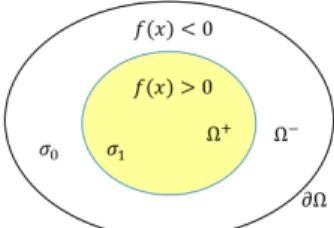
For the sake of brevity, in the following, we assume that there exists a boundaryΓ_⊂Ωthat separates the domainΩinto two regionsΩ−_andΩ+_{, i.e.,Ω = Ω}−S_Ω+_{. The conductivity}

of both regions is assumed to be piecewise constant, i.e.,

σ(x) = σ0 for x ∈ Ω− and σ(x) = σ1 for x ∈ Ω+, as

shown in Fig.1.

The boundaryΓ ={x:f(x) = 0}of the inclusion, which is also an interface between two regions, is presented as the zero level set of a Lipschitz-continuous functionf(x)of dimension

q+ 1 that satisfy      f(x)<0, _∀x_∈Ω−, f(x) = 0, ∀x∈Γ, f(x)>0, _∀x_∈Ω+. (8)

Fig. 1. Illustration of shape representation using a level set function.

Then, the conductivity distribution σ can be represented in terms of LSFf(x)as

σ(x) =σ0(1−H(f(x))) +σ1(H(f(x))), (9)

in which the first term and the last term refer to the background (outside region) and anomaly (inside region) separated by the interface Γ, respectively. Further, H(s) is the Heaviside function, whereH(s) = 0fors <0andH(s) = 1otherwise. In practice, one cannot differentiate the exact Heaviside function in the classical sense, thus one often replaces it with a smooth approximation of the Heaviside function, such as the

C2 _function Hε(s) =    0 s <₋ε, 1 2[1 + s ε+ 1 πsin( πs ε)] |s| ≤ε, 1 s > ε. (10) Here, the parameter ε defines a band Sb = 2ε within which

the Heaviside function is smoothed [54].

To determine the interface Γ, it suffices to determine the LSF f(x). It is clear that many different LSFs can achieve the above requirement, e.g., by applying a signed distance function [43], which is associated with the discretization of x-space. In this paper, we consider now the LSFf(x)expressed parametrically as a linear combination of a predefined basis set as f(x) = N X i=1 µipi(x), (11)

wherepi(x)are the radial basis functions (RBFs) that belong

to the basis set ofP={p1, p2,· · ·pN}.Ndenotes the number

of RBFs andµi, i= 1,2,· · · , N are the weight coefficients.

The shape reconstruction problem is then reduced to the determination of a set of weight coefficients. Consequently, this regime affords the potential to eliminate the requirement of implementing of narrow-band methods [43] and a reini-tialization process that are essential for theTLS approach, where the so-called signed distance function is applied for the LSF and a curve evolution is performed. In addition, well-known properties of the level set approach such as capability and flexibility of handling topology and representing multiple objects are maintained [48]. Possible choices for the P basis function include global RBFs (Gaussian, inverse multi quadric and inverse quadric) and compactly supported RBF (Wend land), etc. A comparison of different RBFs for PLS-based method in EIT, we refer to [55].

In this work, we used Gaussian radial basis function (GRBF) for the basis setP. GRBFs are defined as

pi(x) = exp −k

x₋xik2

2γ2

whereγis the Gaussian width,xiis the RBF center, see details

in Section III-D, and _{k · k}denotes the Euclidean norm. Based on the parameterization of the LSF, equation (8) can be modified as      f(x, µ)< c ∀x∈Ω−, f(x, µ) =c _∀x_∈Γ, f(x, µ)> c ∀x∈Ω+. (13)

Here, c is a small positive value to ensure stable evolu-tion of LSF and µ is the PLS parameter vector, i.e., µ = [µ1, µ2,· · · , µN].

Based on equation (13), the conductivity model in (9) can be expressed as

σ(x, µ) =σ0(1−H(f(x, µ)−c))+σ1(H(f(x, µ)−c)). (14)

This new model in fact maps the space of unknown region

Ω+_{into the space of unknown PLS parameter vectorµ, which}

effectively reduces the dimension and the computational de-mand of the reconstruction problem when the parameterization is chosen properly.

Finally, the observation model in (7) can be updated as

V =U(σ(x, µ)) +e. (15)

For the purposes of clarity, it is important to note that error term e is used herein in a broad sense; in that e given in Eq. 7 is not strictly equivalent to e given in Eq. 15. This realization lies in the fact that the forward modelsU(σ(x, µ))

and U(σ(x)) are not theoretically equivalent and therefore have slightly differing modeling errors. From a pragmatic vantage, these differences we found to be small in comparison to measurement noise and thereby of second-order significance to this work.

C. Extended Kalman filter model

As reported from the Kalman filter approaches studied in [56]–[58], the unknown boundary shape or conductivity distribution is regarded as state variables, whereby the EIT problem is transformed into a state estimation problem. In this work, we treat the unknown state parametersµas a stochastic process which has an evolution model

µk+1 =Fkµk+wk, wk∼ N(0,Γwk), (16)

whereFk ∈RN×N is the state transition matrix and kis the

state index, and wk ∈RN×1 is the evolution noise (assumed

zero mean Gaussian with covariance Γwk). According to the

EIT observation model in (15), for the EIT measurement we write the model

Vk=Uk(µk) +vk, vk∼ N(0,Γvk), (17)

where Vk ∈ RE×1 (E is the number of measurements) is

the vector of measurements at state index k, vk ∈ RE×1 is

the measurement noise (assumed zero mean Gaussian with covariance Γvk) and Uk(µk) denotes the observation model

explain in Section II-A.

In EKF, the nonlinear forward mappingUk(µk)is linearized

ata prioristate estimateµk|k−1at step k,

Vk =Uk(µk|k−1) +Jk µk−µk|k−1

+vk.

(18) The JacobiansJk ∈RE×N will be defined as

Jk =

∂Uk

∂µk|µ

k|k−1. (19)

Let us define the pseudo measurementyk∈RE×1 as

yk≡Vk−Uk(µk|k−1) +Jkµk|k−1. (20)

From equations (18 and 20), we obtain the linearized observation model as

yk=Jkµk+vk. (21)

With the assumptions that the noise is Gaussian and the observation model is linear, the required estimate of µk is

obtained by solving the minimization problem formulated on the basis of (16) and (21) and has the form

ˆ µk= argmin µk n µk−µk|k−1 2 Γ−1 k|k−1 +_kyk−Jkµkk2Γ−1 vk +λ_kI(µk−µ∗)k2 o , (22)

whereΓk|k−1 ∈RN×N is the time-updated error covariance

matrix, λ is the regularization parameter, I ∈ RN×N is the identity matrix and µ∗ _{is a pre-determined vector for the}

unknown state parameter.

If we define the augmented pseudo measurement_eyk and the

augmented pseudo observation matrixHk as

e yk = _y k √ λIµ∗ , (23) and Hk= _J k √ λI . (24)

Then, the minimization problem in (22) can be rewritten as

ˆ µk = argmin µk n µk−µk|k−1 2 Γ−1 k|k−1 +kyek−Hkµkk2Γ−1 k o , (25) where Γ−_k1 _∈ R(E+N)×(E+N) _{is a block diagonal matrix}

defined as

Γ_{k ≡}BlockdiagΓ_vk, I

. (26)

Now the prediction and update steps of the KF can be written as follows.

• Prediction: move the state estimate µk−1|k−1 and its

covarianceΓk−1|k−1 in time

1) Compute µk|k−1=Fk−1µk−1|k−1

2) Compute Γk|k−1=Fk−1Γ_k−1|k−1FkT−1+ Γwk−1 • Update: measurements

1) Compute the Kalman gain Gk =

Γ_k|k−1HT

k(HkΓk|k−1HkT + Γk)−1

2) Compute the updated state estimate µk|k = µk|k−1+Gk(˜yk−Hkµk|k−1)

3) Compute the updated covariance estimate Γk|k =

D. Jacobian calculation

In order to complete the procedure to estimate the unknown state variable (PLS parameter) µin (25), the derivative of the calculated voltageU w.r.tthe state variableµ, i.e., the Jacobian

JU(µ) =∂U_∂µ, is required.

To begin, taking a derivative of conductivityσ(x, µ)in (14)

w.r.tf(x)yields

∂σ

∂f = (σ1−σ0)(δ(f −c)), (27)

whereδ(_·)denotes the Dirac delta function.

Following, the Jacobian JU(µ) = ∂U_∂µ is obtained by

applying the chain rule, yielding

JU(µ) = ∂U ∂σ· ∂σ ∂f· ∂f ∂µ =JU(σ)(σ1−σ0)(δ(f−c)) ∂f ∂µ, (28)

whereJU(σ)can be computed using the standard method, see

details in [59], ∂f_∂µ can be easily computed from (11). III. METHODS

In this section, we describe the models used in the simula-tion studies and the experimental setup.

A. FEM modeling of the human thorax

The geometries of the thorax and lungs were created using EIDORS [60] built-in functions, as shown in the left of Fig. 2. The lungs were simulated as inclusions inside the forward mesh. Note that the inverse meshes were unstructured, i.e., no embedded inclusions were constructed in it. In the forward mesh, the lungs were simulated as varying states by scaling a given 2D lung model with time, such that the numbers of node (Nn) and element (NE) of forward meshes were also

varied, which were around 2000 and 3800, respectively. For the inverse discretization, the numbers of node and element of inverse mesh were fixed, namely,Nn = 1910andNE = 3587.

In the following simulated test cases, L = 16 electrodes (width 1 cm) on the surface of the thorax model were used to acquire conductivity change in lungs. Electric current with amplitude 1 mA was stimulated through adjacent patterns while voltages were measured between adjacent pairs of electrodes. The contact impedances zℓ were set as 0.01 for

all the electrodes.

The assigned conductivities of lung and background were 0.5 mS/cm and 2.0 mS/cm, respectively. In order to simulate inherent noise of EIT systems in reality, we added Gaussian noise with standard deviation 0.1% of the difference between the maximum and minimum value of the noise free mea-surement data to the simulated data. The selected noise level corresponds to the signal to noise (SNR) ratio SNR=45 dB, which represents well the noise level of modern EIT systems [61].

B. Simulation examples

To explore the performance of the PLS-based EKF ap-proach, the following fivetest cases were designed.

• Case 1: Lung imaging without modeling errors. In this case, the model is ideal in the sense that there is no

change of shape of the thorax and the conductivity of lungs. This was done for producing a reference case of lung imaging. As shown in Fig. 2(a), to simulate the lung shape movement, the shape of lungs was changed by linear movement and deformation of the lung boundary, leading to series of changes in the lung area. More specifically, in Fig. 2(a), the outermost solid blue line and the innermost solid cyan line denote the end-inspiration phase and end-expiration phase, respectively. To account for the change in lung cross-sectional area, we calculated the relative area change of lungs (RL):

RL= Area of lungs

Area of lungs at the end-inspiration phase. (29)

The series of RL w.r.t frame number were shown in Fig. 2(c). The simulated scenario contains almost two whole respiratory cycles with 16 frames of thorax images, i.e., end-inspiration phase (RL=1.00) → expiration (RL decreasing) → end-expiration phase (RL=0.64) → end-inspiration phase→end-expiration phase.

(a) changes of lung shape (b) changes of chest domain

(c) Relative changes of lung and chest (d) Conductivity varies in the lung

Fig. 2. Study of lung imaging with and without modeling errors. (a): Geometrical outline of human thorax and lungs. The lungs were simulated as varying states by scaling a given 2D lung model (solid blue line) with time. (b): Shape changes of the thorax in Case 2. (c): Relative changes of lungs and chest domain. (d): Randomly distributed conductivity value of lungs in Case 4, the dashed line indicates the fixedσ1= 0_.6_{mS/cm for the reconstruction.} • Case 2: Lung imaging with modeling errors caused by

changes of the thorax. In clinical situations, the thorax shape varies due to breathing and movements of the thorax. For this reason, we considered a more realistic case in lung imaging. The change of the thorax shape is simulated by linear movement and deformation of the ventral part of the chest. As shown in Fig. 2(b), the outermost solid blue line and the innermost solid black line denote the end-inspiration phase and end-expiration phase, respectively. To account for the level of change, we calculated the relative area change of thorax (RA):

RA= Area of thorax

Area of thorax at the end-inspiration phase. (30)

Again, the series of RA for 16 frames of thorax image were shown in Fig. 2(c). Note that the thorax domain with

RA= 1, corresponding to the end-inspiration phase, was used for solving the inverse problem.

• Case 3: Lung imaging with modeling errors caused by

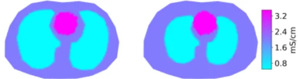
non-homogeneous background. In reality, the conductiv-ity of heart is notably different than the the background tissue. For this reason, we assigned a more realistic conductivity value of 3.5 mS/cm for the heart [62], e.g., two images of the thorax in the end-inspiration phase and the end-expiration phase were shown in Fig. 3. leading to a non-homogeneous background. Namely, the assumption of a constant value ofσ0is violated, leading to modeling

errors in the reconstruction, since only one LSF was applied for representing the conductivity distribution in the model (14).

This test case also provides a chance to investigate the robustness of the propose PLS-based EKF reconstruction with respect to misspecifying the number of phases: The actual target consisted of conductivities in three phases (lungs, heart and background), but in the reconstruction, only two phases (lungs and background) were assumed – by representing the conductivity distribution with one LSF in the model (14). We note that it is possible to apply one more LSF to represent the region of heart, see details in [48] for studying multiphase conductivity reconstruction using PLS method. However, as our pri-mary interest in this study is to evaluate the performance of the PLS-based EKF approach for non-stationary lung imaging, this is out of the scope of the present work. Note that in this case, the thorax shape was fixed as RA=1, and the lung shape evolution follows the same definition in Case 1.

(a) Thorax is in the end-inspiration phase (b) Thorax is in the end-expiration phase

Fig. 3. Two example images of the thorax in the end-inspiration phase and the end-expiration phase with the presence of heart in the background, leading to non-homogeneous background.

• Case 4: Lung imaging with modeling errors caused by varying the conductivity of lungs. In a real situa-tion, the conductivity value of lung varies with inhala-tion and exhalainhala-tion. For this reason, we considered the lungs’ conductivity value as randomly distributed σ1 ∼ N(0.5,0.252_{), as shown in Fig. 2 (d). The minimum and}

maximum conductivity value are 0.54 mS/cm and 0.74 mS/cm, respectively, which are plausible—according to literature [62]. A fixed valueσ0= 0.6mS/cm was applied

for the reconstruction. In addition, same as Case 3, the thorax shape was fixed as RA=1, and the lung shape evolution follows the same definition in Case 1.

• Case 5: Lung imaging with modeling errors caused by varying the conductivity of lungs and changes of the thorax.In a real situation, the lung shape, thorax as well as the conductivity value of lung vary simultaneously with respect to time. For this reason, in Case 5 we

consider both the thorax and the conductivity value of lung behavior to vary simultaneously with respect to time, in which the thorax changes same as in Case 2 and the lungs’ conductivity value assigned in the same way in Case 4. In addition, the lung shape evolution follows the same definition in Case 1. Again, a fixed valueσ0= 0.6 mS/cm and thorax domain with RA= 1

corresponding to the end-inspiration phase were applied in the reconstruction.

In order to simulate a nonstationary environment, it is assumed that a full set of EIT measurements is not available before the lung shape is changed. The current study, therefore, assumed that the lung shape is invariant during the time taken to inject four current patterns and to collect the corresponding voltages. That is, in the EKF reconstruction, at least four states are available for reconstructing a single frame of image. Very often in practice, additional states can be introduced for obtaining better minimization behavior without further measurement data [57]. In other words, for a single frame, four current-voltage data are collected but one or two more states can be introduced, such that the fifth or sixth states are evolved based on the aforementioned four current-voltage data. In this paper, we applied five states per image frame. The additional fifth state was updated based on the fourth current-voltage data. In the present studies, each test case consists of 16 frames of images, which means 64 current injections are applied and 64 EIT data sets are collected, i.e., the whole measurementV _∈R16×64. Then, the number of states evolved for each test case is 80.

C. Experimental studies

The feasibility of the proposed approach was studied exper-imentally. The experiment was carried out using a cylindrical tank shown in Fig. 9. The radius of the tank was 14 cm.

L= 16metallic electrodes with width 2.5 cm were attached to the inner surface of the tank. The tank was filled with saline of conductivity 1.948 mS/cm, and the lung-type inclusions were made of agar. Note that we did not measure the conductivity of lung-likeinclusions, since the exact value of the conductivity after solidification cannot be measured using the conductivity meter.

The EIT measurements were carried out with an in-house system developed in the Department of Modern Physics, Uni-versity of Science and Technology of China.The measurement system takes PXIe-6738 cards supplied by National Instru-ments (NI) as the hardware foundation, and uses the LabView software to realize the data acquisition and compile the control program. The main units of the measurement system are current injection module and voltage measurement module. The current injection module consists of two components: a waveform synthesis unit and a voltage controlled current source. In the waveform synthesis unit, two NI PXI-6733 analog output cards were used to generate sinusoidal voltage signal. Note that, during the design of our measurement system, we followed the well-reported KIT4 system in [63].

The collected data was stimulated with adjacent current pattern (amplitude 1 mA, frequency 10 kHz) and adjacent

measurement. We assumed that a full set of EIT measurements is not available before the lung shape is changed. The current study, therefore, only considered four adjacent current patterns for each single frame of image. In the experiments, the lung-type inclusions are randomly placed in the tank, i.e., at each evolution step the lung position was changing, see details in Fig. 9. To simulate an inspiration state, the sizes of the inclusions were changed after six evolution steps (from T1 to T6 the lung size was fixed, from T6 to T7 the lung size was changing), and then changed again during the eleventh evolution steps (from T7 to T11 the lung size was fixed, from T11 to T12 the lung size was again changing). Note that the conductivity of lung-type inclusions was fixed during the evolution steps.

D. Model implementation

In this section, we discuss important information related the implementation issue of the proposed reconstruction approach. To start, we remark that the initial guess and expected valueµ∗

of the weighting coefficientsµwere set to 0.5 for all studied cases in this paper. Note that the true value of the weight coefficients in each image frame are not known a priori, but they are numerically estimated.

In inverse computation, it was assumed that we do not have the prior knowledge of the evolution therefore the so-called random-walk model is adopted, i.e., Fk = IN ∈ RN×N,

where IN is the identity matrix. The covariance matrices of

the process noise Γωk, measurement noise Γvk and initial

covariance of the predicted errorµ0|0were predetermined and

listed in Table I. In determining these parameters, we utilized trial and error. As for the regularization parameter λ, it was empirically chosen.

To represent the lung shapes, the Heaviside function (10) with ε=_A/2 was applied, here, _A denotes the mean value of the element area in the FEM mesh. The constant c =fm

level set was considered, where fm is the mean value of the

initial LSF fk.

According to relevant works [46], [47], the Gaussian width parameter was defined as γ = _√1

2KA, where K is a free

coefficient of the Gaussian width parameter, which was se-lected based on simulations and visual inspection of the results. In this paper, K was set to 5 and 3/4 for simulated and experimental studies, respectively. For more information regarding the effect of _K to the PLS-based absolute and difference EIT, we refer the reader to our earlier publications [46], [47] for more details.

The PLS-based reconstruction method was found to be quite robust to the selection of locations of RBF centers in [46]. The same selection strategy for RBF centers was used in the study, we chose NRBFc= 31for both simulated and experimental test

cases. Thus, the corresponding unknowns parameters vector was µ ∈R31. Note that the piecewise constant conductivity values in the experimental test case were assumed to be not known a priori; rather, they were estimated together with the

TABLE I

PARAMETERS USED IN THEPLS-BASEDEKFRECONSTRUCTIONS.

Γω_k Γv_k Γ0|0 λ K µ∗

Simulated Cases 0.01IN 5×10−4IE 100IN 1×10−4 5 0.5IN

Experimental Case 0.1IN 5×10−4IE 10IN 1×10−4 3/4 0.5IN

PLS parameter, by solving the minimization problem

[ ˆµk,σˆ0,σˆ1] = argmin n µk−µk|k−1 2 Γ−1 k|k−1 +_keyk−Hkµkk2Γ−1 k + 1 X j=0 k(σj−σj∗)k 2o (31) Here, σ∗

j is a predetermined value of conductivity. More

specifically, we firstly computed the best homogeneous es-timationσd∗

hom∈Rby solving [σd∗

hom] = arg min{kLe(V −U(σhom∗ ))k2}, (32)

here, Le is defined as LTeLe = Ce−1, where Ce is the

observation noise covariance matrix. Then we set σ0∗=σhom∗

andσ∗

1 =14σ∗homfor the experimental reconstruction.

Therefore, in the experimental study, the corresponding unknowns parameters vector was (µ, σ0, σ1) ∈ R33. A

rep-resentative image of the distribution of the RBF centers for both simulated and experimental studies is shown in Fig.4.

(a) Simulated test cases (b) experimental case

Fig. 4. Distributions of the RBF centers.

IV. RESULTS AND DISCUSSIONS

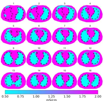
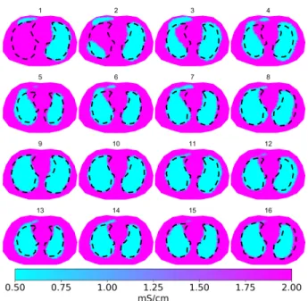
The results of the numerical test cases are shown in Figs. 5-9. In each of these figures, the numbers marked at the top of each sub figure indicate the frame numbers, i.e., each single frame represents the reconstructed image at every fifth state, the dashed line indicates the true shape of lungs, and the PLS-based EKF reconstructions for the moving lung shapes are shown as cyan patches.

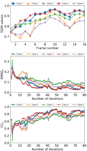
To quantitatively assess the results of the simulated test cases, we computed the structural similarity index (SSIM) [64] for measuring the similarity between the true and reconstructed images. The best SSIM value, 1, would be achieved if and only if the images are identical. When the SSIM value approaches 1, the degree of structural similarity between the two images increases. Note that in Case 3, to avoid the influence arising from the heart region, the true images of Case 1 was used as the reference images for computing the SSIM index, since the main interest in this test case is to recover the lung shapes.

To further quantitatively verify the reconstruction perfor-mances the PLS-based EKF approach, we show the root mean square error (RMSE) and correlation coefficient (CC)

of the estimated conductivity against the iteration steps for the simulated Cases 1-5:

RMSEσ =|| σTrue− Tσˆ|| ||σTrue|| × 100%, (33) and CCσ= (σTrue−σ¯True)T(T(ˆσ−σ¯ˆ)) p ||σTrue−σ¯True||2||σˆ−σ¯ˆ||2 ×100%. (34) Here, _T is a matrix that interpolates the nodal conductivity

ˆ

σ in the inverse mesh into a nodal conductivity σTrue in the

forward mesh. σ¯True and σ¯ˆ are the mean values of σTrue and ˆ

σ, respectively.

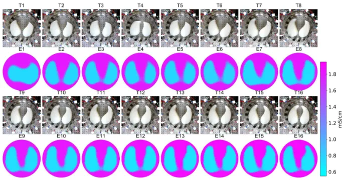
The results of experimental test cases are shown in Fig. 9. In this figure, the real targets were shown in the first and third rows, while the corresponding estimates based on the proposed approach were shown in the second and fourth rows; capital letters ‘T’ and ‘E’ in the subtitles denote the ‘True targets’ and ‘Estimated images’, respectively; the numbers marked at the top of each sub figures indicate the frame numbers.

To quantitatively access the recovery of the binary con-ductivity values and the inclusion shape in the experimental studies, we computed a relative contrast (Rco)

Rco=Estimated conductivity of the background

Measured conductivity of saline , (35) and a size coverage ratio (CR) for measuring how well the sizes of inclusions were recovered:

CR = Estimated inclusion area

True inclusion area ×100%. (36) Half the value of the maximum of the reconstructed con-ductivity, i.e., σ0/2, was used as the threshold for detecting

the inclusions. Note that, the inclusions are irregular shapes, such that the true areas of inclusions are unknown, we use ImageJ [65] to determine the approximated true value. CR value 1 indicates exact match of area of the true and recovered inclusions, while a value less or greater than 1 would indicate underestimation or overestimation of the inclusion area, re-spectively.

A. Results of numerical test cases

1) Case 1: Lung imaging without modeling errors: Fig.5 shows the results of Case 1.We observe that the performance of the proposed is fairly successful, except in early states corresponding to the first few frames of the image where the improper initial guess of the RBFs’ weighting affects the reconstructions. In fact, it is highly unlikely to guess the initial RBFs’ weighting and hence smaller SSIM and higher RMSE values (see details in Fig.10) for the images in the case of the early states are quite probable.

2) Cases 2-5: Lung imaging with modeling errors: Cases 2-5, investigating modeling errors, are shown in Figs. 6-9. In Case 2, due to the change of the thorax shape during the evolution, the reconstructed images are slightly worse compared to the ideal – Case 1. However, except in early states corresponding to the first few frames of the image, the estimated images track the lungs’ shape relatively well, which is also verified by the evaluation metrics plotted in Fig. 10. The

Fig. 5. Case 1: Lung imaging without modeling errors. The sub figures correspond to reconstruction at every fifth states, and numbers marked at the top of each sub figure indicate the frame number; the dashed line indicates the true shape of lungs; the PLS-based EKF reconstructions for the moving lung shapes are shown as cyan patches.

results of Case 2 indicates that the PLS-based EKF approach tolerates inexact knowledge of the body shape.

Fig. 6. Case 2: Lung imaging with modeling errors caused by changes of the thorax. Otherwise as in Fig.5.

In Case 3, where the assumed conductivity phases are less than that are actually present, the reconstructed images are worse compared to that of Cases 1&2, which does not exceed our expectation, due to the modeling errors caused by the non-homogeneous background. Note that, the RMSE and CC values corresponding to most of the iterations in Case 3 are slightly worse than that of other cases; this is also an

intuitively appealing result, because we only apply one LSF for modeling the conductivity distribution, and it is obvious that the heart region can not be tracked, leading to errors in the computation of RMSE and CC. Meanwhile, the results of Case 3 suggest that the PLS-based EKF approach tolerates a misspecification of the phase numbers to some extent – even though the assumed number of phases is too low, the overall quality of the reconstructed image is still quite good.

In Case 4, where the conductivity values of lungs are mis-assigned in the reconstruction, the PLS-based EKF approach yields images with good accuracy, resulting in the evaluation metrics closest to those of the ideal Case 1.

In Case 5, where the thorax as well as the conductivity value of lung vary simultaneously with respect to time, the recon-structions of the lung with PLS-based EKF approach are more affected by the modeling errors, compared to separate Cases 1, 2 & 4, which is also evident from the evaluation criteria shown in Fig. 10. This is mainly due to the fact that mutual influence between the change of thorax shape and varying the lungs’ conductivity adversely affect the reconstruction.

Fig. 7. Case 3: Lung imaging with modeling errors caused by non-homogeneous background. Otherwise as in Fig.5.

Obviously, the modeling errors in all test cases affect the lung shape reconstructions. From these results, we are able to conclude that modeling errors due to the change of thorax shape affected the proposed approach more than other modeling errors. This finding is also supported quantitatively by the evaluation criteria- the worst SSIM of Cases 2 &5 and the worst RMSE and CC of Case 5 (excluding those values of Case 3 affected by the presence of heart) shown in Fig. 10.

Overall, the PLS-based EKF approach yields successful reconstructions of the shape of lungs which even has similar performance compared to the ideal case 1, leading to the trends of SSIM index, RMSE and CC values for Cases 2-5 tend to be somewhat similar to that for Case 1, see Fig. 10. This implies that the PLS-based EKF approach tolerates modeling errors to some extent at least.

Fig. 8. Case 4: Lung imaging with modeling errors caused by varying the conductivity of lungs. Otherwise as in Fig.5.

Fig. 9. Case 5: Lung imaging with modeling errors caused by changes of the thorax and varying the conductivity of lungs. Otherwise as in Fig.5.

Finally, we discuss computational aspects pertinent to the efficiency of the reconstruction algorithm. As an example, the result shown in Fig. 5 was obtained from a MATLAB

implementation on a desktop PC with an Intel Core i7-6700K processor and 32GB memory within 168 seconds at an average speed of 2.10 seconds/state.

B. Results of experimental test case

In the reconstruction, the initial guess of the saline con-ductivity was computed by solving (32). The estimated saline conductivity was estimated to be σd∗

Fig. 10. Comparison of SSIM index, RMSEσ and CC for Cases 1-5.

The reconstructions are shown in Fig. 11. The proposed PLS-based EKF approach is found to track the two targets (lung-like structures) shape and location quite reasonably as observed in Fig. 11. In regard to the estimation of the binary conductivity values, the conductivity of the background is estimated well, which is evident from the relative contrast (Rco), see details in Fig. 12. It should be remarked that we did not compute the Rco value for the targets, since the exact value of the conductivity of the targets after solidification cannot be measured using the conductivity meter. In addition, the coverage ratio (CR) shows that the targets’ area was recovered satisfactorily.

V. DISCUSSION ON THE RESULTS

It is worth remarking that an interesting phenomenon hap-pens in the results of simulated test cases, e.g., from the 13th state to the 16th state in Fig. 6, it seems that the proposed approach could better catch the ‘inner’ boundary of the right lung which is alway from the domain boundary. However, it is very well known that the center of imaging domain has low sensitivity compared to the domain boundary region. The main

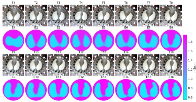
explanation of this phenomenon is that the ‘inner’ boundary changes relatively less than the ‘outer’ boundary, as shown in the top-left of Fig.2, such that EKF-PLS approach is able to substantially track the small changes to the ‘inner’ boundary. In the experimental results, E4 and E6 were quite similar to each other by visual inspection, similar behavior occurred to E11 and E12. One may argue that the experimental results are not quite consistent with the experimental setup. The main reason for this inconsistency is that the changes of lung-shaped inclusions in the experiment are abrupt, such that the difference between the frames is too large and EKF requires some additional states or more transition time to track the inclusion. A potential solution is to consider including more states or adding more process noise for the reconstruction. For example, as shown in Fig. 13, compared to the results in Fig. 11, we applied one more state for each frame, it can be observed that E4 and E6 were different to each other, e.g., the lobe of right ’lung’ moved downward to the right boundary of the tank in E6. Also, for E15 and E16, the lobes of both lungs are moved close to each other, which is consistent with the experimental phenomena.

It is worth mentioning that, in this paper, a random-walk model is used as a state evolution model in which the change between two consecutive states is only governed by the process noise. That is, adding more process noise is another option to represent the feature (e.g., the large difference between the frames) that the state of the shape changes over time. In addition, it is well known that the modeling uncertainty of the random-walk model may cause poor shape reconstruction. To improve the modeling accuracy, dynamic evolution models, e.g., kinematic models, could be used to describe the evolution of the shape. However, studying the selection of optimized initial parameters (e.g., covariance of the process noise) and different evolution models are out of the scope of this paper, therefore, we defer this to future work.

The main application we considered in the study was lung imaging. From a practical point of view, in real time monitoring of lung ventilation, we need to consider modeling error caused by unknown contact impedances, electrode dis-placement, random noise, as well as other unknown auxiliary parameters in the EIT reconstruction problem. For example, in practical measurements the contact impedances are always unknown and can change during the measurement due to sweat on the skin and drying of the electrode gel. This is particularly relevant here, since the proposed approach is based in the context of absolute imaging, which is known to be very sensitive to such kinds of modeling errors [24], [25], [66]. Even though we showed that the proposed approach is tolerant to some of the aforementioned modeling errors to some extent, more practical situations need to be considered. For example: during lung ventilation, conductivity, lung shape, and thorax change simultaneously thereby generating more uncertainty. As a potential solution for handling uncertainties, we suggest applying the so-called approximation error ap-proach [23] to reduce errors intrinsic in the observation model, and to improve the robustness and efficiency of the proposed approach. Another potential solution is to consider extending the current reconstruction framework from the context of

Fig. 11. Case 6: Reconstructions withfivestates per image frame from real water tank data. Capital letters ‘T’ and ‘E’ in the subtitles denote the ‘True targets’ and ‘Estimated images’, respectively.

Fig. 12. Coverage ratio CR and relative contrast Rco versus the frame number in the experimental studies.

absolute imaging to the context ofdifference imaging, which is popularly used in EIT monitoring of lung ventilation, by using a linearization forward model [56]. Clearly, this matter is beyond the scope of this paper and is planned to be studied in future work.

VI. CONCLUSIONS

In this paper, a new parametric level set based EKF ap-proach was proposed for the nonstationary shape reconstruc-tion problem in EIT. It was assumed that the target shape varies during the time taken to collect a full set of independent measurement data. In such transient situations, conventional EIT algorithms based on the static reconstruction may fail to recover the non-stationary conductivity distribution. In order to track the nonstationary target shape, the target boundaries were represented using parametric level set functions, which were decomposed into the weighted summation of radial basis functions, and the weighting coefficients of the radial basis functions were regarded as the unknown state variables. Then, the unknown state variables were estimated with the aid of the EKF. For the verification of the proposed approach, extensive

numerical and experimental test cases were performed and some computational considerations were discussed.

The proposed approach was demonstrated to accurately track the nonstationary target shape relatively well and it was also found to be tolerant to modeling errors caused by inexact knowledge of boundary shape, non-homogeneous background, variation of the piecewise constant conductivity. These findings suggest the PLS-based EKF approach could be used in practical applications of EIT, especially in cases where targets’ topology (e.g., the characteristics of region boundaries)changesduring measurement time.

ACKNOWLEDGMENT

The authors would like to thank Anil Kumar Khambampati, PhD for the helpful discussions. The authors would also like to thank Zhengjie Yu for helping us in carrying out the water tank experiments.

REFERENCES

[1] C. N. Herrera, M. F. Vallejo, J. L. Mueller, and R. G. Lima, “Direct 2-D reconstructions of conductivity and permittivity from EIT data on a human chest,”IEEE Transactions on Medical Imaging, vol. 34, no. 1, pp. 267–274, 2015.

[2] Z. Ren and W. Q. Yang, “Development of a navigation tool for revision total hip surgery based on electrical impedance tomography,” IEEE Transactions on Instrumentation and Measurement, vol. 65, no. 12, pp. 2748–2757, 2016.

[3] Y. Yang, J. Jia, S. Smith, N. Jamil, W. Gamal, and P.-O. Bagnaninchi, “A miniature electrical impedance tomography sensor and 3-d image reconstruction for cell imaging,”IEEE Sensors Journal, vol. 17, no. 2, pp. 514–523, 2017.

[4] Z. Zhao, P.-J. Yun, Y.-L. Kuo, F. Fu, M. Dai, I. Frerichs, and K. M¨oller, “Comparison of different functional eit approaches to quantify tidal ventilation distribution,”Physiological measurement, vol. 39, no. 1, p. 01NT01, 2018.

Fig. 13. Case 6: Reconstructions withsixstates per image frame from real water tank data. Otherwise as in Fig. 11. [5] H. Li, R. Chen, C. Xu, B. Liu, X. Dong, and F. Fu, “Combing

signal processing methods with algorithm priori information to produce synergetic improvements on continuous imaging of brain electrical impedance tomography,”Scientific reports, vol. 8, no. 1, p. 10086, 2018. [6] M. Wang, Q. Wang, and B. Karki, “Arts of electrical impedance tomographic sensing,” Phil. Trans. R. Soc. A, vol. 374, no. 2070, p. 20150329, 2016.

[7] G. Liang, S. Ren, and F. Dong, “Ultrasound guided electrical impedance tomography for 2d free-interface reconstruction,”Measurement Science and Technology, vol. 28, no. 7, p. 074003, 2017.

[8] S. Ren, H. Liu, C. Tan, and F. Dong, “Tomographic wire-mesh imaging of water-air flow based on sparse minimization,”IEEE Sensors Journal, vol. 17, no. 24, pp. 8187–8195, 2017.

[9] D. Smyl, M. Hallaji, A. Sepp¨anen, and M. Pour-Ghaz, “Quantitative electrical imaging of three-dimensional moisture flow in cement-based materials,”International Journal of Heat and Mass Transfer, vol. 103, pp. 1348–1358, 2016.

[10] D. Smyl, M. Pour-Ghaz, and A. Sepp¨anen, “Detection and reconstruction of complex structural cracking patterns with electrical imaging,”NDT & E International, vol. 99, pp. 123–133, 2018.

[11] A. Adler and A. Boyle, “Electrical impedance tomography: Tissue properties to image measures,”IEEE Transactions on Biomedical Engi-neering, vol. 64, no. 11, pp. 2494–2504, 2017.

[12] M. Gevers, P. Gebhardt, S. Westerdick, M. Vogt, and T. Musch, “Fast electrical impedance tomography based on code-division-multiplexing using orthogonal codes,” IEEE Transactions on Instrumentation and Measurement, vol. 64, no. 5, pp. 1188–1195, 2015.

[13] H. Ji, W. Tan, Z. Gui, B. Wang, Z. Huang, H. Li, and G. Wu, “A new dual-modality ect/ert technique based on c4d principle.” IEEE Trans. Instrumentation and Measurement, vol. 65, no. 5, pp. 1042–1050, 2016. [14] Y. Ma, L. Miao, H. Qin, X. Chen, X. Xiong, T. Han, P. Qin, X. Ji, and P. Cai, “A new modular semi-parallel eit system for medical application,”

Biomedical Signal Processing and Control, vol. 39, pp. 416–423, 2018. [15] M. M. Mellenthin, J. L. Mueller, E. D. L. B. de Camargo, F. S. de Moura, T. B. R. Santos, R. G. Lima, S. J. Hamilton, P. A. Muller, and M. Alsaker, “The ace1 electrical impedance tomography system for thoracic imaging,” IEEE Transactions on Instrumentation and Measurement, 2018. [Online]. Available: DOI:10.1109/TIM.2018.2874127

[16] X. Shi, W. Li, F. You, X. Huo, C. Xu, Z. Ji, R. Liu, B. Liu, Y. Li, F. Fu

et al., “High-precision electrical impedance tomography data acquisition system for brain imaging,”IEEE Sensors Journal, vol. 18, no. 14, pp. 5974–5984, 2018.

[17] L. Miao, Y. Ma, and J. Wang, “Roi-based image reconstruction of electrical impedance tomography used to detect regional conductivity

variation,” IEEE Transactions on Instrumentation and Measurement, vol. 63, no. 12, pp. 2903–2910, 2014.

[18] A. Samor`e, M. Guermandi, S. Placati, and R. Guerrieri, “Parametric detection and classification of compact conductivity contrasts with elec-trical impedance tomography,”IEEE Transactions on Instrumentation and Measurement, vol. 66, no. 10, pp. 2666–2679, 2017.

[19] S. Liu, J. Jia, Y. D. Zhang, and Y. Yang, “Image reconstruction in electrical impedance tomography based on structure-aware sparse bayesian learning,” IEEE Transactions on Medical Imaging, vol. 37, no. 9, pp. 2090–2102, 2018.

[20] S. Ren, Y. Wang, G. Liang, and F. Dong, “A robust inclusion bound-ary reconstructor for electrical impedance tomography with geometric constraints,”IEEE Transactions on Instrumentation and Measurement, vol. 68, no. 3, pp. 762–773, 2018.

[21] C. Tan, S. Lv, F. Dong, and M. Takei, “Image reconstruction based on convolutional neural network for electrical resistance tomography,”

IEEE Sensors Journal, vol. 19, no. 1, pp. 196–204, 2019.

[22] D. Liu, D. Gu, D. Smyl, J. Deng, and J. Du, “B-spline based sharp feature preserving shape reconstruction approach for electrical impedance tomography,”IEEE transactions on medical imaging, 2019, in press. [Online]. Available: DOI:10.1109/TMI.2019.2905245 [23] A. Nissinen, V. P. Kolehmainen, and J. P. Kaipio, “Compensation

of modelling errors due to unknown domain boundary in electri-cal impedance tomography,” IEEE Transactions on Medical Imaging, vol. 30, no. 2, pp. 231–242, 2011.

[24] D. Liu, V. Kolehmainen, S. Siltanen, and A. Sepp¨anen, “A nonlinear approach to difference imaging in eit; assessment of the robustness in the presence of modelling errors,”Inverse Problems, vol. 31, no. 3, p. 035012, 2015.

[25] D. Liu, V. Kolehmainen, S. Siltanen, A.-M. Laukkanen, and A. Sepp¨anen, “Nonlinear difference imaging approach to three-dimensional electrical impedance tomography in the presence of geo-metric modeling errors,”IEEE Transactions on Biomedical Engineering, vol. 63, no. 9, pp. 1956–1965, 2016.

[26] X. Dong, C. Tan, and F. Dong, “Gas–liquid two-phase flow velocity measurement with continuous wave ultrasonic doppler and conduc-tance sensor,”IEEE Transactions on Instrumentation and Measurement, vol. 66, no. 11, pp. 3064–3076, 2017.

[27] R. H. Clark, “High-frequency oscillatory ventilation,” in Manual of Neonatal Respiratory Care. Springer, 2017, pp. 337–345.

[28] C. Ermis, A. X. Zhu, S. Pham, J. M. Li, M. Guerrero, A. Vrudney, L. Hiltner, F. Lu, S. Sakaguchi, K. G. Lurie et al., “Comparison of automatic and patient-activated arrhythmia recordings by implantable loop recorders in the evaluation of syncope,”The American journal of cardiology, vol. 92, no. 7, pp. 815–819, 2003.

[29] M. Vauhkonen, P. Karjalainen, and J. Kaipio, “A Kalman filter approach to track fast impedance changes in electrical impedance tomography,”

IEEE Transactions on Biomedical Engineering, vol. 45, no. 4, pp. 486– 493, 1998.

[30] V. Kolehmainen, A. Voutilainen, and J. P. Kaipio, “Estimation of non-stationary region boundaries in eit—state estimation approach,”Inverse Problems, vol. 17, no. 6, p. 1937, 2001.

[31] K. Kim, B. Kim, M. Kim, Y. Lee, and M. Vauhkonen, “Image recon-struction in time-varying electrical impedance tomography based on the extended kalman filter,”Measurement Science and Technology, vol. 12, no. 8, p. 1032, 2001.

[32] A. Sepp¨anen, M. Vauhkonen, P. Vauhkonen, E. Somersalo, and J. Kaipio, “State estimation with fluid dynamical evolution models in process tomography-an application to impedance tomography,” Inverse Prob-lems, vol. 17, no. 3, p. 467, 2001.

[33] F. C. Trigo, R. Gonzalez-Lima, and M. B. P. Amato, “Electrical impedance tomography using the extended kalman filter,”IEEE Trans-actions on Biomedical Engineering, vol. 51, no. 1, pp. 72–81, 2004. [34] A. Voutilainen, A. Lipponen, T. Savolainen, A. Lehikoinen, M.

Vauhko-nen, and J. P. Kaipio, “Fast adaptive 3-d nonstationary electrical impedance tomography based on reduced-order modeling,”IEEE Trans-actions on Instrumentation and Measurement, vol. 61, no. 10, pp. 2665– 2681, 2012.

[35] A. K. Khambampati, K. Y. Kim, Y.-G. Lee, and S. Kim, “Boundary element method to estimate the time-varying interfacial boundary in horizontal immiscible liquids flow using electrical resistance tomogra-phy,”Applied Mathematical Modelling, vol. 40, no. 2, pp. 1052–1068, 2016.

[36] A. Adler, T. Dai, and W. R. Lionheart, “Temporal image reconstruc-tion in electrical impedance tomography,”Physiological measurement, vol. 28, no. 7, p. S1, 2007.

[37] H. Gagnon, B. Grychtol, and A. Adler, “A comparison framework for temporal image reconstructions in electrical impedance tomography,”

Physiological measurement, vol. 36, no. 6, p. 1093, 2015.

[38] A. Lipponen, A. Sepp¨anen, and J. Kaipio, “Electrical impedance tomog-raphy imaging with reduced-order model based on proper orthogonal decomposition,” Journal of Electronic Imaging, vol. 22, no. 2, pp. 023 008–023 008, 2013.

[39] A. Rashid, S. Kim, D. Liu, and K. Kim, “A dynamic oppositional biogeography-based optimization approach for time-varying electrical impedance tomography,”Physiological measurement, vol. 37, no. 6, p. 820, 2016.

[40] D. Watzenig, M. Brandner, and G. Steiner, “A particle filter approach for tomographic imaging based on different state-space representations,”

Measurement Science and Technology, vol. 18, no. 1, p. 30, 2006. [41] A. Khambampati, A. Rashid, B. Kim, D. Liu, S. Kim, and K. Kim, “Em

algorithm applied for estimating non-stationary region boundaries using electrical impedance tomography,” inJournal of Physics: Conference Series, vol. 224, no. 1. IOP Publishing, 2010, p. 012044.

[42] A. Rashid, B. Kim, A. Khambampati, S. Kim, and K. Kim, “An oppo-sitional biogeography-based optimization technique to reconstruct organ boundaries in the human thorax using electrical impedance tomography,”

Physiological measurement, vol. 32, no. 7, p. 767, 2011.

[43] M. Soleimani, W. Lionheart, and O. Dorn, “Level set reconstruction of conductivity and permittivity from boundary electrical measurements using experimental data,”Inverse problems in science and engineering, vol. 14, no. 2, pp. 193–210, 2006.

[44] M. Y. Wang and S. Wang, “Parametric shape and topology optimization with radial basis functions,” inIUTAM symposium on topological design optimization of structures, machines and materials. Springer, 2006, pp. 13–22.

[45] A. Aghasi, M. Kilmer, and E. L. Miller, “Parametric level set methods for inverse problems,”SIAM Journal on Imaging Sciences, vol. 4, no. 2, pp. 618–650, 2011.

[46] D. Liu, A. K. Khambampati, and J. Du, “A parametric level set method for electrical impedance tomography,”IEEE Transactions on Medical Imaging, vol. 37, no. 2, pp. 451–460, 2018.

[47] D. Liu, D. Smyl, and J. Du, “A parametric level set based approach to difference imaging in electrical impedance tomography,”IEEE transac-tions on medical imaging, vol. 38, no. 1, pp. 145–155, 2019. [48] D. Liu, Y. Zhao, A. K. Khambampati, A. Seppanen, and J. Du, “A

parametric level set method for imaging multi-phase conductivity using electrical impedance tomography,”IEEE Transactions on Computational Imaging, vol. 4, no. 4, pp. 552–561, 2018.

[49] J. Ye, H. Wang, Y. Li, and W. Yang, “Coupling of fluid field and elec-trostatic field for electrical capacitance tomography,”IEEE Transactions

on Instrumentation and Measurement, vol. 64, no. 12, pp. 3334–3353, 2015.

[50] I. Ismail, J. Gamio, S. A. Bukhari, and W. Yang, “Tomography for multi-phase flow measurement in the oil industry,”Flow Measurement and Instrumentation, vol. 16, no. 2-3, pp. 145–155, 2005.

[51] W. Warsito and L.-S. Fan, “Measurement of real-time flow structures in gas–liquid and gas–liquid–solid flow systems using electrical capac-itance tomography (ect),”Chemical Engineering Science, vol. 56, no. 21-22, pp. 6455–6462, 2001.

[52] E. Somersalo, M. Cheney, and D. Isaacson, “Existence and uniqueness for electrode models for electric current computed tomography,”SIAM Journal on Applied Mathematics, vol. 52, no. 4, pp. 1023–1040, 1992. [53] P. Vauhkonen, M. Vauhkonen, T. Savolainen, and J. Kaipio, “Three-dimensional electrical impedance tomography based on the complete electrode model,” IEEE Trans. Biomed. Eng, vol. 46, pp. 1150–1160, 1999.

[54] G. Pingen, M. Waidmann, A. Evgrafov, and K. Maute, “A parametric level-set approach for topology optimization of flow domains,” Struc-tural and Multidisciplinary Optimization, vol. 41, no. 1, pp. 117–131, 2010.

[55] D. Liu, D. Smyl, and J. Du, “Comparison of different radial basis functions for parametric level set based method in electrical impedance tomography,” in9th World Congress on Industrial Process Tomography (WCIPT9), Bath, UK.

[56] M. Vauhkonen, P. Karjalainen, and J. Kaipio, “A Kalman filter ap-proach applied to the tracking of fast movements of organ boundaries,”

Proceedings of the 20th Annual International Conference of the IEEE Engineering in Medicine and Biology Society., vol. 20, no. 2, pp. 1048– 1051, 1998.

[57] S. Kim, U. Z. Ijaz, A. K. Khambampati, K. Y. Kim, M. C. Kim, and S. I. Chung, “Moving interfacial boundary estimation in stratified flow of two immiscible liquids using electrical resistance tomography,”Measurement Science and Technology, vol. 18, no. 5, pp. 1257–1269, 2007. [58] S. Kim and A. K. Khambampati, Mathematical concepts for image

reconstruction in tomography. Elsevier Ltd, 2015.

[59] M. Vauhkonen, D. Vadasz, P. A. Karjalainen, E. Somersalo, and J. P. Kaipio, “Tikhonov regularization and prior information in electrical impedance tomography,”IEEE transactions on medical imaging, vol. 17, no. 2, pp. 285–293, 1998.

[60] A. Adler and W. R. Lionheart, “Uses and abuses of eidors: an extensible software base for eit,”Physiological measurement, vol. 27, no. 5, p. S25, 2006.

[61] J. Avery, T. Dowrick, M. Faulkner, N. Goren, and D. Holder, “A versa-tile and reproducible multi-frequency electrical impedance tomography system,”Sensors, vol. 17, no. 2, p. 280, 2017.

[62] C. Gabriel, A. Peyman, and E. Grant, “Electrical conductivity of tissue at frequencies below 1 mhz,”Physics in medicine and biology, vol. 54, no. 16, p. 4863, 2009.

[63] J. Kourunen, T. Savolainen, A. Lehikoinen, M. Vauhkonen, and L. Heikkinen, “Suitability of a pxi platform for an electrical impedance tomography system,” Measurement Science and Technology, vol. 20, no. 1, p. 015503, 2009.

[64] Z. Wang, A. C. Bovik, H. R. Sheikh, and E. P. Simoncelli, “Image quality assessment: from error visibility to structural similarity,”IEEE transactions on image processing, vol. 13, no. 4, pp. 600–612, 2004. [65] C. A. Schneider, W. S. Rasband, and K. W. Eliceiri, “Nih image to

imagej: 25 years of image analysis,”Nature methods, vol. 9, no. 7, p. 671, 2012.

[66] D. Liu, V. Kolehmainen, S. Siltanen, A. M. Laukkanen, and A. Sepp¨anen, “Estimation of conductivity changes in a region of interest with electrical impedance tomography,”Inverse Problems and Imaging, vol. 9, no. 1, pp. 211–229, 2015.