HAL Id: hal-01964720
https://hal.archives-ouvertes.fr/hal-01964720v3
Preprint submitted on 27 Jan 2020
HAL is a multi-disciplinary open access archive for the deposit and dissemination of sci-entific research documents, whether they are pub-lished or not. The documents may come from teaching and research institutions in France or
L’archive ouverte pluridisciplinaire HAL, est destinée au dépôt et à la diffusion de documents scientifiques de niveau recherche, publiés ou non, émanant des établissements d’enseignement et de recherche français ou étrangers, des laboratoires
Imputation and low-rank estimation with Missing Not
At Random data
Aude Sportisse, Claire Boyer, Julie Josse
To cite this version:
Aude Sportisse, Claire Boyer, Julie Josse. Imputation and low-rank estimation with Missing Not At Random data. 2020. �hal-01964720v3�
Imputation and low-rank estimation with Missing Not At
Random data
Aude Sportissea,c, Claire Boyera,b, Julie Jossec,d
aLaboratoire de Probabilités Statistique et Modélisation, Sorbonne Université, France b
Département de Mathématiques et applications, Ecole Normale Supérieure, Paris, France
c
Centre de Mathématiques Appliquées, Ecole Polytechnique, France
d
XPOP, INRIA, France
Abstract
Missing values challenge data analysis because many supervised and unsu-pervised learning methods cannot be applied directly to incomplete data. Matrix completion based on low-rank assumptions are very powerful solu-tion for dealing with missing values. However, existing methods do not con-sider the case of informative missing values which are widely encountered in practice. This paper proposes matrix completion methods to recover Miss-ing Not At Random (MNAR) data. Our first contribution is to suggest a model-based estimation strategy by modelling the missing mechanism dis-tribution. An EM algorithm is then implemented, involving a Fast Iterative Soft-Thresholding Algorithm (FISTA). Our second contribution is to sug-gest a computationally efficient surrogate estimation by implicitly taking into account the joint distribution of the data and the missing mechanism: the data matrix is concatenated with the mask coding for the missing val-ues; a low-rank structure for exponential family is assumed on this new matrix, in order to encode links between variables and missing mechanisms. The methodology that has the great advantage of handling different missing value mechanisms is robust to model specification errors.
The performances of our methods are assessed on the real data collected from a trauma registry (TraumaBaseR) containing clinical information about over twenty thousand severely traumatized patients in France. The aim is then to predict if the doctors should administrate tranexomic acid to patients with traumatic brain injury, that would limit excessive bleeding.
Keywords: Informative missing values, denoising, matrix completion, accelerated proximal gradient method, EM algorithm, nuclear norm penalty.
1. Introduction
The problem of missing data is ubiquitous in the practice of data analysis. Main approaches for handling missing data include imputation methods and the use of Expectation-Maximization (EM) algorithm [8] which allows to get the maximum likelihood estimators in various incomplete-data problems [24]. The theoretical guarantees of these methods ensuring the correct prediction of missing values or the correct estimation of some parameters of interest are only valid if some assumptions are made on how the data came to be missing. Rubin [34] introduced three types of missing-data mechanisms: (i) the restrictive assumptions of missing completely at random (MCAR) data, (ii) the missing at random (MAR) data, where the missing data may only depend on the observable variables, and (iii) the more general assumption of missing not at random (MNAR) data,i.e. when the unavailability of the data depends on the values of other variables and its own value. A classic example of MNAR data, which is the focus of the paper, is surveys where rich people would be less willing to disclose their income or where people would be less incline to answer sensitive questions on their addictive use. Another example would be the diagnosis of Alzheimer’s disease, which can be made using a score obtained by the patient on a specific test. However, when a patient has the disease, he or she has difficulty answering questions and is more likely to abandon the test before it ends.
Missing non at random data. When data are MCAR or MAR, valid infer-ences can be obtained by ignoring the missing-data mechanism [24]. The MNAR data lead to selection bias, as the observed data are not represen-tative of the population. In this setting, the missing-data mechanism must be taken into account, by considering the joint distribution of complete data matrix and the missing-data pattern. There are mainly two approaches to model the joint distribution using different factorizations:
1. selection models [15], which seem preferred as it models the distribution of the data, sayY, and the incidence of missing data as a function of Y which is rather intuitive;
2. pattern-mixture models [23], which key issue is that it requires to spe-cify the distribution of each missing-data pattern separately.
Most of the time, in these parametric approaches, the EM algorithm is per-formed to estimate the parameters of interest, such as the parameters of
generalized linear models in [16] and the missing-data mechanism distribu-tion is usually specified by logistic regression models [16,37,30], in the case of selection models. In addition, the MNAR mechanism often is chosen self-masked i.e. the lack of a variable depends only on the variable itself and only simple models have been considered with cases where just the output variable or one or two variables are subject to missingness [27, 16]. Note that recent works based on graph-based approaches [28, 29] show that in some specific setting of MNAR values, it is possible to estimate parameters for simple models, such as the mean and variance in linear models, without specifying the missing value mechanism.
Low-rank models with missing values. In this paper, we focus on estimation and imputation in low-rank models with MNAR data. The low-rank model has become very popular in recent years [21] and it plays a key role in many scientific and engineering tasks, including denoising [9], collaborative filtering [42], genome-wide studies [22,32], and functional magnetic resonance imag-ing [7]. It is also a very powerful solution for dealing with missing values [18, 20]. Indeed, the low-rank assumption can be considered as an accurate approximation for many matrices as detailed in [39]. For instance, the low-rank approximation makes sense when either, one can consider that a limited number of individual profiles exist or, dependencies between variables can be established.
Let us consider a data matrix Y ∈ Rn×p which is a noisy realisation of a
low-rank matrixΘ∈Rn×p with rank r <min{n, p}:
Y = Θ +,where
Θhas a low rank r,
∼ N(0, σ2I). (1)
In the following, σ is assumed to be known. Suppose that only partial observations are accessible. We note the maskΩ∈ {0,1}n×p with
Ωij =
0 if yij is missing,
1 otherwise.
where y is a realisation of Y. The main objective is then to estimate the parameter matrixΘfrom the incomplete data, which can be seen on the one hand as a denoising task by estimating the parameters from the observed incomplete noisy data, and on the other hand as a prediction task by im-puting missing values with values given by the estimated parameter matrix. A classical approach to estimateΘwith MAR or MCAR missing values are based on convex relaxations of the rank, i.e. the nuclear norm and consists in solving the following penalized weighted least-squares problem:
ˆ
Θ∈argminΘk(Y −Θ)Ωk2F +λkΘk?, (2) wherek.kF andk.k? respectively denote the Frobenius norm and the nuclear
norm and is the Hadamard product. The main algorithm available to solve (2) consists in a proximal gradient method, leading to iterative soft-thresholding algorithm (ISTA) of the singular value decomposition (SVD) [26, 3] in the case of a regularization via the nuclear norm (note that this strategy is equivalent to perform an EM algorithm with a nuclear norm penalization in the M-step, see AppendixB.2). Given any initialization (for instance the missing values can be initialized to the mean of the non-missing entries), a soft-thresholding SVD is computed on the completed matrix and the predicted values of the missing entries are updated using the values given by the new estimation. The two steps of estimation and imputation are iterated until empirical stabilization of the prediction. There has been a lot of work on denoising and matrix completion with low-rank models, whether algorithmic, methodological or theoretical contributions [6,5]. However, to the best of our knowledge most of the existing methods do not consider the case of MNAR data.
Contributions. In order to perform low-rank estimation with MNAR data, our first contribution, detailed in Section 3.1, is to suggest a model-based estimation strategy by maximizing the joint distribution of the data and the missing values mechanism using an EM algorithm. More specifically, a Monte Carlo approximation is performed coupled with the Sampling Im-portance Resampling (SIR) algorithm. Note yet that introducing such a model for MNAR data does not prevent from handling Missing Completely At Random (MCAR) or Missing At Random (MAR) data as well. Indeed, our model can only impact variables of type MNAR, while the low-rank assumption will be enough to deal with other types of missing variables. This approach, although theoretically sound and well defined, has two draw-backs: its computational time and the need to specify an explicit model for the mechanism, so to have a strong prior knowledge about the shape of the missing-data distribution.
Our second contribution (Section3.2) is to suggest an efficient surrogate es-timation by implicitly modelling the joint distribution. To do so, we suggest to concatenate the data matrix and the missing-data mask,i.e. the indicator matrix coding for the missing values, and to assume a low-rank structure on this new matrix in order to take into account the relationship between the variables and the mechanism. This strategy has the great advantage that it can be performed using classical methods used in the MCAR and MAR
settings and that it does not require to specify a model for the mechanism. This approach can be seen as connected to the following works. [11] presents a method to handle missing data in a latent-class model where the missing covariatesX are linked to the missing-data pattern M by a latent variable η. In an example, they suggests treatingM as additional items alongsideX, in order to make statistical inferences. Moreover, in the context of decision trees used for classification, [38] suggests an approach known as missing val-ues attribute where at each split, all the missing valval-ues can go on the right or on the left. This can be seen as cutting according to the missing value pattern so it is equivalent as implicitly adding M with the covariates X. Finally, from the optimization point of view, we also suggest (Section 3.3) to use an accelerated proximal gradient algorithm, also called Fast Iterative Soft-Thresholding Algorithm (FISTA) [2] which is an accelerated version of the classical iterative SVD algorithm in the case of a penalization with the nuclear norm.
The rest of the article is organized as follows. First, although the missing-data mechanism framework is widely used, there are points of ambiguity in the classical definitions, especially considering whether the statements hold for any value (from any sample) or for the realised value (from a specific sample) [36,31]. Therefore, Section 2 is dedicated to specify a general and clear framework of the missing-data mechanisms in order to remove ambigui-ties and introduce the MNAR mechanism being considered. In Section3, we present both proposals to address the MNAR data issue: by explicitly mod-elling the missing mechanism or by implicitly taking it into account. Section
4is devoted to a simulation study on synthetic data. In Section5, we apply the model-based method to the TraumaBaseR dataset in order to to assist doctors in making decisions about the administration of an active substance, called the tranexomic acid, to patients with traumatic brain injury. Finally, a discussion on the results and perspectives is proposed on Section6.
2. The missing-data mechanism: notations and definitions
In the sequel, we write the complete data matrixY ∈Rn×p of quantitative
variables, whose distribution is parameterized by Θ. The missing-data pat-tern is denoted byM ∈ {0,1}n×p and φis the parameter of the conditional
distribution ofM given Y. We assume the distinctness of the parameters,
i.e. the joint parameter space of(Θ, φ)is the product of the parameter space of Θand the one of φ. We start by writing the most popular definitions of [24] for the missing-data mechanism. By writing, Y = (Yobs, Ymis), where
Yobs and Ymis denote the observed components and the missing ones of Y
respectively, they define:
p(M|Y;φ) =p(M;φ), ∀Y, φ (MCAR)
p(M|Y;φ) =p(M|Yobs;φ), ∀Ymis, φ (MAR)
p(M|Y;φ) =p(M|Yobs, Ymis;φ), ∀φ (MNAR)
Note that all matrices may be regarded as vectors of sizen×p (see Exam-ple 2.1). There are mainly two ambiguities: (i) it is unclear whether the equations hold for any realisation(y, m) of(Y, M), although it is widely un-derstood as such and (ii)Yobs and Ymis are actually functions of M, which
is extremely confusing and explain why other attempts for definitions and notations are necessary. [36] propose two definitions of the MAR mechanism, for which they differentiate if (i) the statements hold for any values (from any sample), the everywhere case (EC) (ii) or for the realised values (from a specific sample), the realised case (RC). They also introduce a specific nota-tion for the observed values ofY, clearly written as a functionoofY andM: o(Y, M). By writing y˜and m˜ the realised values ofY and M for a specific sample, it leads to:
∀y, y∗, msuch thato(y, m) =o(y∗, m)
p(M =m|Y =y;φ) =p(M =m|Y =y∗;φ), (EC)
∀y, y∗ such thato(y,m) =˜ o(y∗,m) =˜ o(˜y,m)˜
p(M = ˜m|Y =y;φ) =p(M = ˜m|Y =y∗;φ), (RC) We can illustrate these concepts with the following example:
Example 2.1. Let y=
1 3
4 10
, that can be regarded as a vectorvec(y) = 1 3 4 10
. Ifvec(y) = 1 3 4 NA
is observed, thenm˜ = 1 1 1 0 ando(˜y,m) = 1˜ 3 4. The data are realised MAR if
p(M = (1,1,1,0)|Y =y;φ) =p(M = (1,1,1,0)|Y =y∗;φ), ∀y, y∗, o(y,m) =˜ o(y∗,m) = (1,˜ 3,4) m p(M = (1,1,1,0)|Y = (1,3,4, a);φ) =p(M = (1,1,1,0)|Y = (1,3,4, b);φ),∀a, b
By extending the framework of [36], the MNAR mechanism can be defined in the everywhere case and with the two following assumptions:
• the missing-data indicators are independent given the data,
• the MNAR mechanism is said to be self-masked, which assures that the distribution of a missing-data indicatorMij given the data Y is a
function ofYij only.
In the specific case of low-rank models, these both assumptions allow to have the independence by unit and to make the computations easier.
Definition 2.1. The missing data are generated by the self-masked every-where MNAR mechanism if:
p(M = Ω|Y =y;φ) = n Y i=1 p Y j=1 p(Ωij|yij;φ), ∀Y, φ 3. Proposition
Our propositions for low-rank estimation with MNAR data require the fol-lowing comments on the classical algorithms to solve (2). First, as in re-gression analysis there is an equivalence between minimizing least-squares and maximizing the likelihood under Gaussian noise assumption. Here as specified in Equation (1), the entries(Yij)ij’s are assumed to be independent
and normally distributed, for alli∈[1, n], j∈[1, p]:
p(yij; Θij) = (2πσ2)−1/2e −1 2 yij−Θij σ 2 . (3)
It implies that we can show (in Appendix B.2) that the classical proximal gradient methods to solve the penalized weighted least-squares criterion (2), such as iterative thresholding SVD, can be seen as a genuine EM algorithm, maximizing the observed penalized likelihood. Second, as detailed in Sec-tion3.3, (2) can be solved using a fast iterative soft-thresholding algorithm (FISTA) [2].
3.1. Modelling the mechanism
Considering the framework of selection models [15], the first proposition consists in handling MNAR values in the low-rank model (1), by specifying a distribution for the missing-data patternM. Here, the missing data models
Mij given the data Yij are assumed to be independent and distributed by a
logistic model,∀i∈[1, n],∀j∈[1, p]:
p(Ωij|yij;φ) = [(1 +e−φ1j(yij−φ2j))−1](1−Ωij)
[1−(1 +e−φ1j(yij−φ2j))−1]Ωij, (4) whereφj = (φ1j, φ2j)denotes the parameter vector for conditional
distribu-tion ofMij givenYij for all i.
Then, the joint distribution of the data and mechanism can be specified. Due to independence (see Definition (2.1)):
p(y,Ω; Θ, φ) =p(y; Θ)p(Ω|y;φ) = n Y i=1 p Y j=1 p(yij; Θij)p(Ωij|yij;φj).
This leads to the joint negative log-likelihood:
`(Θ, φ;y,Ω) =− n X i=1 p X j=1 `((Θij, φj);yij,Ωij),
with `((Θij, φ);yij,Ωij) = log(p((yij,Ωij); Θij, φj)), ∀i, j. In practice, the
parameters vector φis unknown but viewed as a nuisance parameter, since our main interest is the estimation ofΘ. To find an estimatorΘˆ, we aim at maximizing the following penalized joint negative log-likelihood:
( ˆΘ,φ)ˆ ∈argminΘ,φ`(Θ, φ;y,Ω) +λkΘk?. (5) It can be achieved using a Monte-Carlo Expectation Maximization (MCEM) algorithm, whose two steps, iteratively proceeded, are given below:
• E-step: the expectation (taking the distribution of the missing data given the observed data and the missing-data pattern) of the complete data likelihood is computed:
Q(Θ, φ|Θˆ(t),φˆ(t)) =EYmis h `(Θ, φ;y,Ω)|Yobs, M; Θ = ˆΘ(t), φ= ˆφ(t) i (6)
• M-step: the parametersΘˆ(t+1) and φˆ(t+1) are determined as follows: ˆ
The E-step may be rewritten as follows: Q(Θ, φ|Θˆ(t),φˆ(t)) = − n X i=1 p X j=1 CΩij 1 + C 1−Ωij 2 where C1 = log(p(yij,Ωij; Θij, φj)) C2 = Z log(p(yij,Ωij; Θij, φj))p(yij|Ωij; ˆΘ(ijt),φˆ (t) j )dyij
Note that the E-step is written as a sum of the E-steps for each (i, j)-th elements. If the (i, j)-th element is observed, we do not integrate and it leads to the first term; the second term corresponds to the missing elements. By the lack of a closed form for Q, it is approximated by using a Monte Carlo approximation, denoted asQˆ,∀i∈[1, n],∀j∈[1, p]:
ˆ Qij(Θ, φ|Θˆ(t),φˆj (t) ) = − 1 Ns Ns X k=1 log(p(vijk; Θij)) + log(p(Ωij|vijk;φj)), wherevkij = yij if Ωij = 1, zkij otherwise, withz k
ij the realisation ofZ ∼p(yij|Ωij; ˆΘ(ijt),φˆj
(t)
). Note thatQˆ is separable in the variablesΘandφ, so that the maximization for the M-step may be independently performed forΘandφ:
ˆ Θ(t+1) ∈argmin Θ n X i=1 p X j=1 1 Ns Ns X k=1 −log(p(vijk; Θij)) +λkΘk? (8) ˆ φ(t+1) ∈argmin φ n X i=1 p X j=1 1 Ns Ns X k=1 −log(p(Ωij|vijk;φj)). (9)
Classical algorithms can be used: (accelerated) proximal gradient method to solve (8) and the Newton-Raphson algorithm to solve (9).
Moreover, for all i∈ {1, . . . , n} and j ∈ {1, . . . , p} such that yij is missing,
we suggest the use of the sampling importance resampling (SIR) algorithm [10] to simulate the variablezijk. The detail is given in AppendixC.1and we take as a proposal distribution a Gaussian distribution.
3.2. Adding the mask
We now propose to directly include the information of the mask while con-sidering the criterion (2), without explicitly modelling the mechanism, so that the new optimisation problem is written as follows:
ˆ
Θ∈argminΘ1
2k[ΩY|Ω]−[Ω|1][Θ|Ω]k
2
F +λkΘk?, (10)
where1 ∈Rn×p denotes the matrix such that all its elements are equal to
1, and [X1|X2] denotes the column-concatenation of matrices X1 and X2.
To solve (10), we could use again classical algorithms such as the (acceler-ated) iterative (SVD) soft-thresholding algorithm (Section 3.3). However, this approach does not take into account that the mask is made of binary variables and suggests that the concatenated matrix[Y Ω,Ω] is Gaussian. Consequently, a better approach is to take into account the mask binary type by using the low-rank model but extended to the exponential family. There is a vast literature on how to deal with mixed matrices (containing categorical, real and discrete variables) in the low-rank model, see for exam-ple [40, 25, 4]. [33] suggested such a method, by using a data-fitting term based on heterogeneous exponential family quasi-likelihood with a nuclear norm penalization: ˆ Θ∈argminΘ n X i=1 p X j=1 Ωij(YijΘij +gj(Θij)) +λkΘk?, (11)
where gj is a link function chosen according to the type of the variable j.
In our case, it allows to model the joint distribution of the concatenated matrix [Y Ω,Ω] of size n×2p as follows : (i) the data are assumed to be Gaussian, i.e. for all j ∈ [1, p], gj(x) = x
2σ2
2 (ii) the missing-data pattern
can be modelled by the Bernoulli distribution with success probability1/(1+ exp(−Θij)), i.e. for all j ∈ [p+ 1,2p], gj(x) = log(1 + exp(x)). To solve
(11), a Penalized Iteratively Reweighted Least Squares algorithm calledmimi (see [33, page 12]) is used. The advantage of such a strategy is to better incorporate the mask as binary features but this comes at a price of a more involved algorithm in comparison to (10).
3.3. FISTA algorithm
To solve (2), (8) and (10) we suggest to use the FISTA algorithm, introduced by [2], detailed in AppendixA, which corresponds to an accelerated version
of the proximal gradient method. The acceleration is performed via momen-tum. The key advantage is that it converges to a minimizer at the rate of
O(1/K2) (K is the number of iterations) in the case of L-smooth functions.
This algorithm is of interest compared to the the non-accelerated proxi-mal gradient method, that is shown in AppendixB.1 to be implemented in softImpute-SVDin the R packagesoftImpute(see [12]): it is known to con-verge only to the rateO(1/K)[2, Theorem 3.1]. To be more precise, another algorithm has been suggested that uses alternating least-squares [13] and de-parts from the previous one by solving a non-convex problem: it relies on the maximum margin matrix factorization approach (combined with a final SVD thresholding). Therefore, although appealing numerically, the algo-rithm known as softImpute-ALSis proven to converge only to a stationary point.
4. Simulations
The parameterΘis generated as a low-rank matrix of sizen×pwith a fixed rankr <min(n, p). The results are presented forN simulations, for each of them: (i) a noisy versionY ofΘis considered,
Y = Θ +,
whereis a Gaussian noise matrix with i.i.d. centered entries of varianceσ2, (ii) MNAR missing values are introduced using a logistic regression, resulting in a mask Ω and (iii) only knowing Y Ω, we apply different methods to denoise and impute Y:
(a) Explicit method (Model): in order to take into account the missing mechanism modelling, we apply the MCEM algorithm to solve (5), as detailed in Section3.1; note that either FISTA orsoftImpute are performed in the M-step.
(b) Implicit method (Mask): the missing mechanism is implicitly inte-grated by concatenating the mask to the data, as detailed in Sec-tion 3.2. When the binary type of the mask is neglected, FISTA or softImpute are used to solve (10). When taking into account the binary type of the mask, solving (11) is done by mimi.
(c) MAR methods: they consist in classical methods for low-rank matrix completion, proved to be efficient under the MCAR or MAR assump-tion, and that aim at minimizing (2). The missing values mechanism is then ignored. They encompass FISTA andsoftImpute.
We also include in(b)and(c)the regularised iterative PCA algorithm [41,18] which uses another penalty than the nuclear norm one. We also compare all the methods to the naive imputation by the mean (the estimation of Θ is obtained by replacing all values by the mean of the column). We performed an extended simulation study and other more heuristic methods have been tested, such as the FAMD and MFA algorithms dedicated to mixed data or blocks of variables [1] but they are not included in the article to make the plots more readable as the results were never convincing. The results presented are representative of all the results obtained.
The results are presented for different matrix dimensions and ranks, mech-anisms of missing values (MAR and MNAR), and percentages of missing data. The code to reproduce all the simulations is available on github https://github.com/AudeSportisse/stat.
Measuring the performance. To measure the methods performance, two types of normalized mean square errors (MSE) are considered:
E ( ˆΘ−Y)(1−Ω) 2 F , E h kY (1−Ω)k2Fi (12) E Θˆ −Θ 2 F , E h kΘk2Fi, (13)
that are respectively the prediction error, corresponding to the error commit-ted when we impute values, and the total error, encompassing the prediction and the estimation error.
Some practical details on the algorithms are provided in the following para-graphs.
EM algorithm. The stopping criterion used in the EM algorithm is the fol-lowing:
kΘˆ(t)−Θˆ(t−1)kF kΘˆ(t−1)k
F +δ ≤τ,
whereδ = 10−3 and τ = 10−21. In addition, the E-step is performed with Ns = 1000 Monte Carlo iterations. The key issue of this method is the
run-time complexity largely due to this Monte Carlo approximation.
1
Once the stopping criterion is met,T = 10 extra iterations are performed to assure the convergence stability.
Tuning the algorithms hyperparameters. When considering (2), (10) and (7), the regularisation parameter λ is chosen among some fixed grid G =
{λ1, . . . , λM} to minimize either the prediction or the total errors. In the
regularised iterative PCA algorithm, the hyper-parameter is the number of components to perform PCA, which can be found using cross-validation crite-ria. In the simulations, the noise level is assumed to be known. To overcome this hypothesis, one can use standard estimators of the noise level such as the ones of [9] and [18].
4.1. Univariate missing data
Let us consider a simple case with n = 100 and p = 4, the rank of the parameter matrix isr = 1 andσ2 = 0.8. Assume that only one variable has
missing entries. The missing values are introduced by using the self-masked MNAR mechanism. The missingness probabilities are then given as follows:
∀i∈[1 :n], p(Ωi1 = 0|yi1;φ) =
1
1 +e−φ1(yi1−φ2) (14)
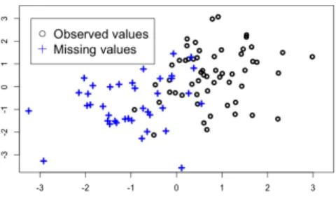
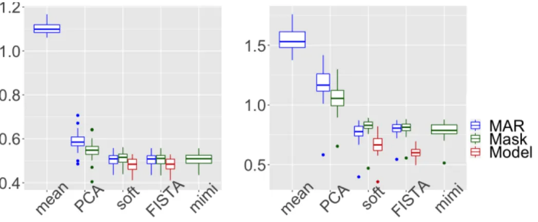
The parameters of the logistic regression are chosen to mimic a cutoff effect, see Figure 1. Indeed, extrapolating imputed values can be challenging and classical methods are expected to introduce a large prediction bias. Given the previous parameters choice, the percentage of missing values is 50% in expectation for the missing variable, corresponding to12.5% missing values in the whole matrix. In Figure 2, the three methods (a), (b) and (c) are compared in such a setting, using boxplots on MSE errors forN = 50 simu-lations. In this MNAR setting, the proposed model-based method(a), in red in Figure2, aiming at minimizing (5) -specially designed for such a setting-gives better results globally for the total error with a significant improve-ment on the prediction of missing values (either when FISTA orsoftImpute is used in the M-step of the MCEM algorithm).
In addition, the implicit methods (b), in green in Figure 2, working on the concatenation of the mask and the data, either based on a binomial modeling of the mechanism (mimi, solving (11)), or neglecting the binary feature of the mask (FISTA and softImpute, solving (10)), do not lead to improved performance compared to the MAR method (c) (FISTA and softImpute) in terms of prediction or estimation errors. On the contrary, the implicit method(b) working on the concatenation of the mask and the data, based now on the regularized iterative PCA improves both estimation and predic-tion errors compared to the regular PCA algorithm used in the MAR method
(c). However the obtained prediction error does not compete with perfor-mance of regular MAR completion algorithms (FISTA andsoftImpute).
Figure 1: Introduction of MNAR missing values using a logistic regression (14), with φ1= 3andφ2= 0. One can see that the the highest values ofyi1 are missing, mimicking
a cutoff effect.
Note also that the results of both SVD algorithms,softImputeand FISTA, are similar in terms of estimation and prediction error, but FISTA has the advantage to improve the numerical convergence to a minimizer.
In conclusion on the univariate case, (i) modelling the missing mechanism outperforms any other method, particularly in terms of prediction error; (ii) implicit methods (b) have limited interest, except to improve the regular PCA algorithm.
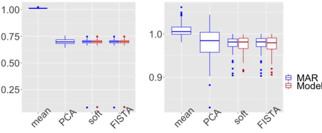
4.2. Bivariate missing data
We consider now a higher dimensional case: n = 100 and p = 50 and the rank of the parameter matrix is r = 4. The noise level is σ2 = 0.8, as in Section (4.1). The missing values are introduced on two variables by using the following MNAR mechanism, for alli∈[1, n]and j∈[1,2],
p(Ωij = 0|yij;φ) = 1 1 +e−φ1j(yij−φ2j) where φ1j = 3, φ2j = 0 if j= 1, φ1j = 2, φ2j = 1 if j= 2.
This parameters choice leads to 50% missing values in Y.1 and 20% in Y.2
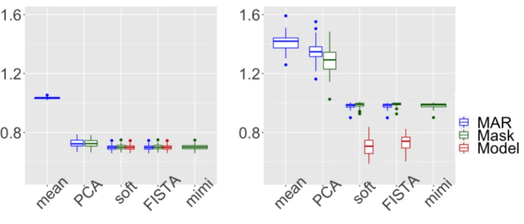
mimicking a cutoff effect again. In Figure 3, the methods (a), (b) and (c)
are compared in such a setting, using boxplots on MSE errors for N = 50 simulations.
The model-based method (a), designed for the MNAR setting, give signifi-cant better results than any other method in terms of prediction error. The
Figure 2: Univariate missing data: total error (left) and prediction error (right) for the methods(a)in red,(b)in green and(c)in blue.
mask-adding methods (b) lead to no significant improvement compared to classical MAR methods, either by solving (10) using FISTA,softImpute, or solving (11) via mimi. One can note that the PCA algorithm still benefits from the concatenation with the mask in terms of prediction error, but to a lesser extent than in the univariate case.
Overall, the poor performance of the mask-adding methods (b) can be ex-plained by the dimensionality issue and the small weight of the added mask variables. Indeed, in this higher dimensional case with bivariate missing variables, only two informative binary variables corresponding to the mask are really concatenated to a 50-column matrix.
Note that in terms of total error, the advantages of model-based methods
(a)are no longer visible, which can be explained by the very low percentage of missing data (1.5%) (see Section 4.3 in which more missing values are considered).
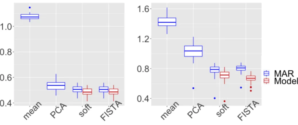
4.3. Multivariate missing data
We consider now a multivariate missing data case for the following dimen-sional setting: n = 100, p = 20 and r = 4. The missing values are in-troduced on ten variables by using the following MNAR mechanism, for all i, j∈[1, n]×[1,10],
p(Ωij = 0|yij;φ) =
1
Figure 3: Bivariate missing data: total error (left) and prediction error (right) for the methods(a)in red,(b)in green and(c)in blue.
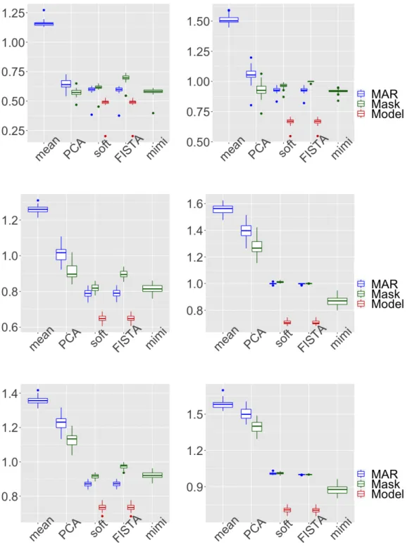
Note that the parameters of the missingness mechanism are the same for each element, this can be easily extended to a more general case. The parameters choice leads to 25% missing values in the whole matrix. The results are presented in Figure 4 for N = 50 simulations and different noise levels, σ2= 0.2,0.5 or 0.8.
First, one can note that the model-based method(a)provides the best result both in estimation and prediction error regardless the noise level (and what-ever FISTA orsoftImputeused in the MCEM). Of course, this performance improvement comes at the price of a computational cost due to the Monte Carlo approximations needed in the MCEM algorithm.
Regarding the implicit methods (b), the mask-adding techniques handling the concatenation of the data and the mask matrix as Gaussian (FISTA and softImpute) miss to improve both estimation and prediction errors com-pared to their MAR version. However, the variantmimimodelling the mask with a binomial distribution always largely outperforms MAR methods (c)
in terms of prediction (while the improvement in terms of estimation error is only visible at a low noise level). Therefore, the mask-adding approach can implicitly capture the MNAR missing mechanism, when the mask is re-ally considered as a matrix of binary variables. This comes at the price of a more involved algorithm mimi able to take into account mixed variables, but that remains far less computationally expensive than the model-based approach. Indeed, for an estimation/prediction of one parameter matrixΘ, the process time for a computer with a processor Intel Core i5 of 2,3 GHz is
0.0549 seconds for the MAR method withsoftImpute, 3.215 seconds for the implicit method withmimi and 13.069 minutes for the model-based method withsoftImputewhen50% of the variables are missing.
As a side comment, in this high-dimensional setting, one can note that the PCA algorithm still benefits from adding the mask, which is a variant of method (b), compared to the regular PCA method, both in estimation and prediction error. However the mask-adding PCA algorithm only com-pete the mask-adding methods based on iterative SVD thresholding (FISTA, softImpute) at a low noise level.
4.4. Sensitivity to model misspecifications
Deviation in the missing-data mechanism setting. Here, the missing values are introduced by using the MAR mechanism. It allows to test the stability of model-based methods, designed for the MNAR setting, to a deviation in the missing mechanism. The missingness probabilities are given as follows in such a setting:
∀i∈[1, n], p(Ωi1 = 0|yi2;φ) =
1
1 +e−φ1(yi2−φ2), (15)
meaning that the probability to have a missing value in Y1 depends on the
value ofY2.
First, let us consider the setting of Section 4.1, i.e. n= 100,p= 4,r= 1. In Figure 5, we observe that the model-based method (a) improves both the estimation and the prediction, which is not expected in a MAR setting. However, this can be explained because of the rank is one which implies that there are only small differences between MNAR and MAR (the second variable’s value is directly linked to the missing one’s value). Consequently, modelling a MNAR mechanism is enough to retrieve information on such a MAR missing mechanism.
To avoid this case, we consider the setting of Section4.2, i.e.n= 100,p= 50, r = 4, with a MAR missing mechanism as described by (15), however, the second variable involved is chosen to be decorrelated from the missing one (which is possible given the rank is4). In such a case, there is no equivalence between the missing values that are simulated to be MAR and the mechanism we model as MNAR. Figure 6 shows that the model-based approach does not lead to any improvement compared to regular methods used for MAR methods; but more importantly, it does not degrade the results either which highlights the robustness of the approach with respect to deviations from the model.
Figure 4: Multivariate MNAR missing data: total error (left) and prediction error (right) for the methods(a)in red,(b)in green and(c). Three noise settings are considered: on top strong signal (σ2= 0.2), middle noisy data (σ2= 0.5), bottom very noisy data (σ2= 0.8).
Figure 5: Comparison of methods performance when the missing data are of type MAR (forN = 50 simulations) with a rank one: total error (left) and prediction error (right) for different methods and algorithms.
Figure 6: Comparison of methods performance when the missing data are of type MAR (forN= 50simulations) with a rank four (the MAR mechanism depends on a decorrelated variable to the missing one): total error (left) and prediction error (right) for different methods and algorithms.
Figure 7: Univariate MNAR missing data parametrized with a probit model forN = 50simulations: total error (left) and prediction error (right) for different methods and algorithms. Note that the methods modeling the missing mechanisms use the logistic model.
Deviation in the logistic regression setting. We now want to test the ro-bustness of our model-based method(a)to a misspecification of the logistic model, given by (4). To do so, missing values are introduced by a MNAR data mechanism based on the following probit model, the missing-ness probabilities are then:
∀i∈[1, n], p(Ωi1= 0|yi1;φ) =F(yi1),
whereF is the quantile function the standard Gaussian cumulative distribu-tion funcdistribu-tion. Consider the setting of Secdistribu-tion4.1, i.e. n= 100,p= 4,r = 1. In Figure7, we observe that the model-based methods(a)globally improves the results for both errors (13) and (12). Very similar results to the ones of Section4.1are obtained, meaning that the model-based method(a)behaves well to a deviation of the logistic regression modelling.
5. Application to clinical data
5.1. Motivation
Our work is motivated by a public health application with APHP TraumaBaseR2 Group (Assistance Publique - Hopitaux de Paris) on the management of
matized patients. Major trauma, i.e. injuries that endanger a person’s life or functional integrity, have been qualified as a worldwide public health chal-lenge and a major source of mortality (first cause in the age group 16-45) in the world by the WHO [14]. Hemorrhagic shock and traumatic brain injury have been identified as the lead causes of death. Effective and timely man-agement of trauma is crucial to improve outcomes, as delays or errors entail high risks for the patient.
5.2. Data description
A subset of the trauma registry containing the clinical measurements of3168 patients with brain trauma injury is first selected.
Our aim is to predict from pre-hospital measurements whether or not the tranexomic acid3 should be administrated on arrival at the hospital. In the dataset, the variableTranexomic.acid is the decision made by the doctors, which is considered as ground truth. This variable is equal to1if the doctors have decided to administrate tranexomic acid,0 otherwise.
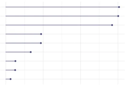
Nine quantitative variables containing missing values are selected by doctors. In Figure 8, one can see the percentage of missing values in each variable, varying from1.5to 30%, leading to 11%is the whole dataset. After discus-sion with doctors, almost all variables can be considered to have informative missingness. For example, when the patient’s condition is too critical and therefore his heart rate (variableHR.ph) is either high or low, the heart rate may not be measured, as doctors prefer to provide emergency care. The heart rate itself can then be qualified of self-masked MNAR, and the other variables, either of MNAR or MAR. Both percentage and nature of missing data demonstrate the importance of taking appropriate account of missing data. More information on the data can be found in AppendixD.
In the following, two questions are addressed. Firstly, we compare the valid-ity of the imputation methods in terms of prediction of the tranexomic acid administration based on the different imputed data. Secondly, we test the methods in terms of their imputation performance.
5.3. Prediction of administration of the tranexomic acid
We consider a two-step procedure:
• Step 1: imputation of the explanatory variables. As a preprocessing step, we impute missing data in the explanatory variables, beforehand
HR.ph SBP.ph DBP.ph Shock.index.ph Delta.shock.index Sp02.min HemoCue.init Delta.hemoCue Cristalloid.volume 0 10 20 30 % Missing V ar iab les
Figure 8: Percentage of missing values in each variable.
proceeding to the classification training. Imputation is performed us-ing the model-based method(a), the implicit methods(b)or the MAR methods(c). All these methods are compared to the naive imputation by the mean.
• Step 2: classification task which consists in predicting the administra-tion or not of the tranexomic acid. Therefore, we are looking for the prediction functionf such that
Z 'f(Yimp),
whereZ ∈ {0,1}nis equal to 1 (resp. 0) if the tranexomic acid is (resp.
not) administered, and Yimp ∈ Rn×p represents the nine imputed
ex-planatory variables discussed above. Based on these new-filled design matrices formed in Step 1, the classification is always done using either random forests or logistic regression.
Since not administering tranexomic acid by mistake can be vital, for the training and testing errors, we use a dissymetrized loss function where the cost of false negatives is much more than of false positives
as follows l(ˆz, z) = 1 n n X i=1 w01{zi=1,zˆi=0}+w11{zi=0,ˆzi=1}, (16)
wherew0 andw1are the weights for the cost of false negative and false
positive respectively, s.t. w0+w1 = 1 andω0= 5ω1.
The dataset is divided into training and test sets (random selection of80−
20%) and the prediction quality on the test set is compared according to different indicators such as the accuracy, the sensitivity, etc.
Table 1 compares results when random forests are used as a prediction method. In this setting, mean imputation gives among the best results on all the metrics which is in agreement with recent results on its consistency when used with a powerful learner, see Josse et al. [19]. Nevertheless, the model-based method(a)is very competitive. The proposed implicit methods result in the best performances in terms of the sensitivity which is particularly relevant for the application.
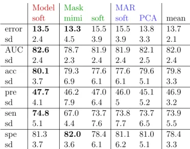
Table 2 compares results when the prediction is performed with logistic re-gression. For almost all criteria, and especially on sensitivity the model-based method (a) leads to the best performances. The standard deviations are also smaller with the model based approach in comparison with the im-plicit methods.
Therefore, the model-based method performs well regardless of the prediction method used.
5.4. Imputation performances
As the methods are initially designed for imputation, we perform simula-tions on the real dataset. In order to be able to measure the quality of the imputation, some additional MNAR values are introduced in the variable
Shock.index.ph, which is a variable with MNAR missing values (according to doctors) that contains initially7% of missing values. The missing values are introduced by using the self-masked mechanism described in (14). The choice of parameters in the logistic regression leads to 35% missing values. In the model-based method (a), the variables are scaled before each EM it-eration to give the same weight to each variable. Besides, the noise level σ2 is estimated using the residual sum of squares divided by the number of observations minus the number of estimated parameters as suggested in [18],
ˆ
σ2 = kY −
Pr
l=1uldlvlk22
Model Mask MAR
soft mimi soft soft PCA mean
error 12.5 16.0 15.8 14.8 13.6 13.0 sd 3.3 2.8 4.9 5.0 3.2 2.1 AUC 85.4 83.9 84.6 84.6 85.5 85.2 sd 1.6 1.7 1.8 2.0 1.4 2.2 acc 79.5 77.8 77.6 78.6 79.9 80.7 sd 5.0 3.2 5.0 5.2 3.4 3.1 pre 47.5 45.0 45.1 46.5 45.2 48.7 sd 6.7 4.2 8.2 8.3 5.9 5.0 sen 76.5 78.1 78.2 77.4 72.4 76.0 sd 6.1 3.4 5.7 5.4 3.2 4.5 spe 80.2 77.7 77.4 78.9 80.8 81.7 sd 7.2 4.4 7.2 7.3 4.6 4.6
Table 1: By using random forest for the classification. Comparison of the mean of different prediction criteria over ten simulations (values are multiplied by 100). Error corresponds to the validation error with the loss described in (16). AUC is the area under ROC; the accuracy (acc) is the number of true positive plus true negative divided by the total number of observations; the sensitivity (sen) is defined as the true positive rate; specificity (spe) as the true negative rate; the precision (pre) is the number of true positive over all positive predictions. The lines sd correspond to standard deviations. The three best results are in bold.
Model Mask MAR
soft mimi soft soft PCA mean
error 13.5 13.3 15.5 15.5 13.8 13.7 sd 2.4 4.5 3.9 3.9 3.3 2.1 AUC 82.6 78.7 81.9 81.9 82.1 82.0 sd 2.4 2.3 2.4 2.4 2.5 2.4 acc 80.1 79.3 77.6 77.6 79.6 79.8 sd 3.7 6.9 6.1 6.1 5.1 3.3 pre 47.7 46.2 47.0 46.0 45.1 46.9 sd 4.1 7.9 6.4 5 5.2 3.2 sen 74.8 67.0 73.7 73.8 73.7 73.9 sd 5.1 4.4 7.6 7.7 6.5 5.5 spe 81.3 82.0 78.4 81.1 81.0 78.4 sd 3.7 3.6 6.1 6.2 5.1 3.3
Table 2: By using logistic regression for the classification. Comparison of the mean of different prediction criteria over ten simulations (values are multiplied by 100). Error corresponds to the validation error with the loss described in (16). AUC is the area under ROC; the accuracy (acc) is the number of true positive plus true negative divided by the total number of observations; the sensitivity (sen) is defined as the true positive rate; specificity (spe) as the true negative rate; the precision (pre) is the number of true positive over all positive predictions. The lines sd correspond to standard deviations. The two best results are in bold.
0.3
0.4
0.5
0.6
0.7
mean
PCA
soft
mimi
MAR
Mask
Model
Generic
Figure 9: Comparison of the imputation error (for ten simulations).
where ul, vl and dl are the singular vectors and the singular values from
the singular value decomposition of Y. We let r denote the rank of Y, estimated here using cross-validation [17]. In Figure 9, the three methods
(a), (b) and (c) are compared using boxplots of the prediction error over ten simulations. The proposed method(a), designed for the MNAR setting, gives significantly smaller prediction error than other methods. Besides, the other proposed methods (b), taking the mask into account, also improve prediction errors compared to the classical MAR methods(c).
6. Discussion
In this article two methods have been suggested for handling self-masked MNAR data in the low-rank context: explicit modeling of the mechanism or implicit consideration by adding the mask. The first method is clearly the most successful in terms of prediction or estimation errors. Moreover, it is robust to model misspecifications. However, one should note that, on the one hand it can be computationally expensive, and then hardly scalable in the high-dimensional multivariate missing setting and on the other hand, it is a parametric approach. Therefore, the implicit method handling both the data and the mask matrices, when taking into account the binary distribution of the latter, may be regarded as the right alternative. Both methods can handle MNAR and MAR data simultaneously.
As a take-home message, one should keep in mind that (i) if there are a few missing variables, the model-based method is extremely relevant; and (ii)
when many variables can be missing, the implicit method, that models the mask using a binomial distribution, has empirically proven to provide better imputation.
Note that the logistic regression assumption may seem restrictive but the proposed approach could be easily adapted to other distributions such as the probit one.
We pointed out that when the rank is one, there are few differences between MAR and MNAR, which implies that MNAR missing values could be han-dled without specifiying a model. This is in line with the work of [29] in regression using graphical models and it would be interesting to extend their work to low-rank models.
As directions of future research, one could also extend this work to data matrices containing mixed variables (quantitative and categorical variables) with MNAR data, so that the logistic regression model should include the case of categorical explanatory and output variables.
In addition, in this paper, we focus on single imputation techniques where a unique value is predicted for each missing value. Consequently, it can not reflect the variance of prediction. It would be very interesting to derive con-fidence intervals for the predicted value, for instance by considering multiple imputation methods [35].
Acknowledgments
The authors are thankful for fruitful discussion with François Husson, Wei Jiang, Imke Mayer and Geneviève Robin.
Appendices
A. The FISTA algorithmWe first present the proximal gradient method. The following optimisation problem is considered:
ˆ
Θ∈argminΘh1(Θ) +h2(Θ),
whereh1 is a convex function, h2 a differentiable and convex function and
Algorithm 1Proximal gradient method Step 0: Θˆ(0) the null matrices.
Step t+ 1: Θˆ(t+1)=proxλ(1/L)h
1( ˆΘ
(t)−(1/L)∇h
2( ˆΘ(t)))
The main trick of the FISTA algorithm is to add a momentum term to the proximal gradient method, in order to yield smoother trajectory towards the convergence point. In addition, the proximal operator is performed on a specific linear combination of the previous two iterates, rather than on the previous iterate only.
Algorithm 2FISTA (accelerated proximal gradient method) Step 0: κ0= 0.1,Θˆ(0) andΞ0 the null matrices.
Step t+ 1: ˆ Θ(t+1)=proxλ(1/L)h1(Ξt−(1/L)∇h2(Ξt)) κk+1= 1+√1+4κ2 k 2 Ξt+1 = ˆΘ(t+1)+κκk−1 k+1( ˆΘ (t+1)−Θˆ(t))
In our specific model, to solve (2), h1(Θ) =kΘk? and h2(Θ) = kΩ(Θ−
Y)k2
F. Let us precise that:
∂h2(Θ) ∂Θij =∇Θijh2(Θ) = Ωij(Θij−Yij). Therefore, ∇h2(Θ) = Ω(Θ−Y) andL is equal to 1. B. softImpute
We start by describingsoftImpute. Algorithm 3softImpute
Step 0: Θˆ(0) the null matrix. Step t+ 1: Θˆ(t+1)=prox
λk.k?(ΩY + (1−Ω)Θˆ(t))
The proximal operator of the nuclear norm of a matrixX consists in a soft-thresholding of its singular values: we perform the SVD ofX and we obtain
the matricesU,V and D. Then
proxλk.k?(X) =U DλV.
Dλ is the diagonal matrix such that for all i,
Dλ,ii= max((σi−λ),0)
, where the(σii)’s are the singular values ofX.
B.1. Equivalence between softImputeand the proximal gradient method
By using the same functionsh1 andh2 as above, one has:
ˆ
Θ(t+1)=proxλ(1/L)h1( ˆΘ(t)−(1/L)∇h2( ˆΘ(t)))
=proxλk.k?( ˆΘ(t)−Ω( ˆΘ(t)−Y)) =proxλk.k?(ΩY + (1−Ω)Θˆ(t)),
so thatsoftImputeand the proximal gradient method are similar.
B.2. Equivalence between the EM algorithm and iterative SVD in the MAR case
We prove here that in the MAR setting, softImpute is similar to the EM algorithm. Let us recall that in the MAR setting the model of the joint distribution is not needed but only the one of the data distribution, so that the E-step is written as follows:
Q(Θ|Θˆ(t)) =EYmis h log(p(Θ;y))|Yobs; Θ = ˆΘ (t)i ∝ − n X i=1 p X j=1 E " yij−Θij σ 2 |Θˆij(t) # ,
by using (3) and the independance ofYij,∀i, j). Then, by splitting into the observed and
the missing elements,
Q(Θ|Θˆ(t) )∝ − n X i=1 X j,Ωij=0 E " yij−Θij σ 2 |Θˆij(t) # − n X i=1 X j,Ωij=1 yij−Θij σ 2
Therefore, Q(Θ|Θˆ(t))∝ − n X i=1 X j,Ωij=0 E[y2ij−2Θijyij+ Θ2ij|Θˆij (t) ]2 − n X i=1 X j,Ωij=1 yij−Θij σ 2 Q(Θ|Θˆ(t))∝ − n X i=1 X j,Ωij=0 σ2+ ˆΘij (t)2 −2 ˆΘij (t) Θij+ Θ2ij − n X i=1 X j,Ωij=1 yij−Θij σ 2 which impliesQ(Θ|Θˆ(t))∝ kΩY + (1−Ω)Θˆ(t)−Θk2 F The M-step is then written as follows:
ˆ
Θ(t+1) ∈argminΘkΩY + (1−Ω)Θˆ(t)−Θk2F +λkΘk?
The proximal gradient method is applied with
h1(Θ) =λkΘk? andh2(Θ) =kΩY + (1−Ω)Θˆ(t)−Θk2F.
Therefore, the EM algorithm in the MAR case is the same one assoftImpute.
C. The EM algorithm in the MNAR case
For the sake of clarity, we present below the EM algorithm in the MNAR and low dimension case.
Algorithm 4The EM algorithm in the MNAR case Step 0: Θˆ(0) andφˆ(0).
Step t+ 1:
for(i, j)∈Ωmis ={(l, k), l∈[1, n], k∈[1, p],Ωlk= 0} do
draw z1ij, . . . , zNs
ij i.i.d.
∼ hyij|Ωij; ˆφ(t),Θˆ(ijt) i
with the SIR algorithm. end for
Compute Θˆ(t+1) by using softImputeor the FISTA algorithm with the imputed matrixV (given by (17)).
Compute φˆ(t+1) by using the function glm with a binomial link, which perform a logistic regression of J.(1j) on J.(2j), with the matrix J(j) given
We already have given details for the stopping criterium. We clarify the maximization step given by (8) and (9).
ˆ Θ∈argmin Θ X i,j 1 Ns Ns X k=1 1 2σ2(v (k) ij −Θij)2 ! +λkΘk? ∈argmin Θ X i,j 1 Nsσ2 Ns X k=1 −vij(k)Θij+ 1 2Θ 2 ij ! +λkΘk? ∈argmin Θ kV −Θk2 F +λkΘk?, where: V = 1 Ns PN s k=1v (k) 11 . . .N1s PN s k=1v (k) 1p .. .. .. ... 1 Ns PN s k=1v (k) n1 . . . 1 Ns PN s k=1v (k) np (17) ˆ φ(t+1)∈argmin φ X i,j 1 Ns Ns X k=1 (1−Ωij)C3−ΩijC4 ∈argmin φ X i,j 1 Ns Ns X k=1 C3+ Ωijφ1j(vijk −φ2j) with: C3 = log(1 +e−φ1j(v k ij−φ2j)) C4 = log(1−(1 +e−φ1j(v k ij−φ2j))−1)
For all j ∈ {1, . . . , p} such that ∃i ∈ {1, . . . , n}, Ωij = 0, estimating the
coefficients φ1j and φ2j remains to fit a generalized linear model with the
binomial link function for the matrixJ(j):
J(j)= Ω1j v(1)1j .. . ... Ωnj v(1)nj .. . ... Ω1j v1(Njs) .. . ... Ωnj vnj(Ns) (18)
C.1. SIR
In the Monte Carlo approximation, the distribution of interest is
h
yij|Ωij; ˆφj(t),Θˆ(ijt) i
. By using the Bayes rules:
p yij|Ωij; ˆφj(t),Θˆ(ijt) =:f(yij) ∝pyij; ˆΘ(ijt) pΩij|yij; ˆφ(jt) =:g(yij)
Denoting the Gaussian density function of mean Θ(ijt) and variance σ2 by
ϕ
Θ(ijt),σ2, if σ >(2π)
−1/2, the following condition holds:
f(yij) =cg(yij)≤ϕΘ(t)
ij,σ2 (x). ForM large, the SIR algorithm to simulate
z∼hyij|Ωij; ˆφj(t),Θˆ(ijt) i
is described as follows. Algorithm 5SIR
Draw: a sample x1, . . . , xM ∼ N(Θ(ijt), σ2).
Compute the weights:
ω(xm) = g(xm) ϕΘ(t) ij,σ2 (xm) , for m= 1, . . . , M.
Drawzfrom the original samplex1, . . . , xM with probability proportional
to ω(x1), . . . , ω(xM).
D. Details on the variables in TraumaBaseR
A description of the variables which are used in Section 5 is given. The indications given in parentheses ph (pre-hospital) and h (hospital) mean that the measures have been taken before the arrival at the hospital and at the hospital.
• SBP.ph, DBP.ph, HR.ph: systolic and diastolic arterial pressure and heart rate during pre-hospital phase. (ph)
• HemoCue.init: prehospital capillary hemoglobin concentration. (ph)
• SpO2.min: peripheral oxygen saturation, measured by pulse oxymetry, to estimate oxygen content in the blood. (ph)
• Cristalloid.volume: total amount of prehospital administered cristal-loid fluid resuscitation (volume expansion). (ph)
• Shock.index.ph: ratio of heart rate and systolic arterial pressure during pre-hospital phase. (ph)
• Delta.shock.index: Difference of shock index between arrival at the hospital and arrival on the scene. (h)
• Delta.hemoCue: Difference of hemoglobin level between arrival at the hospital and arrival on the scene. (h)
References
[1] Vincent Audigier, François Husson, and Julie Josse. A principal com-ponent method to impute missing values for mixed data. Advances in Data Analysis and Classification, 10(1):5–26, 2016.
[2] Amir Beck and Marc Teboulle. A fast iterative shrinkage-thresholding algorithm for linear inverse problems. SIAM journal on imaging sciences, 2(1):183–202, 2009.
[3] Jian-Feng Cai, Emmanuel J Candès, and Zuowei Shen. A singular value thresholding algorithm for matrix completion. SIAM Journal on Optimization, 20(4):1956–1982, 2010.
[4] Tony Cai and Wen-Xin Zhou. A max-norm constrained minimization approach to 1-bit matrix completion. The Journal of Machine Learning Research, 14(1):3619–3647, 2013.
[5] Emmanuel J Candes and Yaniv Plan. Matrix completion with noise. Proceedings of the IEEE, 98(6):925–936, 2010.
[6] Emmanuel J Candès and Benjamin Recht. Exact matrix completion via convex optimization. Foundations of Computational mathematics, 9(6):717, 2009.
[7] Emmanuel J Candès, Carlos A Sing-Long, and Joshua D Trzasko. Un-biased risk estimates for singular value thresholding and spectral es-timators. IEEE Transactions on Signal Processing, 61(19):4643–4657, 2013.
[8] Arthur P Dempster, Nan M Laird, and Donald B Rubin. Maximum likelihood from incomplete data via the em algorithm. Journal of the Royal Statistical Society: Series B (Methodological), 39(1):1–22, 1977. [9] Matan Gavish and David L Donoho. Optimal shrinkage of singular
values. IEEE Transactions on Information Theory, 63(4):2137–2152, 2017.
[10] Neil J Gordon, David J Salmond, and Adrian FM Smith. Novel ap-proach to nonlinear/non-gaussian bayesian state estimation. In IEE Proceedings F-radar and signal processing, volume 140, pages 107–113. IET, 1993.
[11] Ofer Harel and Joseph L Schafer. Partial and latent ignorability in missing-data problems. Biometrika, 96(1):37–50, 2009.
[12] Trevor Hastie and Rahul Mazumder. softImpute: Matrix Completion
via Iterative Soft-Thresholded SVD, 2015. URL https://CRAN.
R-project.org/package=softImpute. R package version 1.4.
[13] Trevor Hastie, Rahul Mazumder, Jason D Lee, and Reza Zadeh. Matrix completion and low-rank svd via fast alternating least squares. The Journal of Machine Learning Research, 16(1):3367–3402, 2015.
[14] Simon I Hay, Amanuel Alemu Abajobir, Kalkidan Hassen Abate, Cris-tiana Abbafati, Kaja M Abbas, Foad Abd-Allah, Rizwan Suliankatchi Abdulkader, Abdishakur M Abdulle, Teshome Abuka Abebo, Se-maw Ferede Abera, et al. Global, regional, and national disability-adjusted life-years (dalys) for 333 diseases and injuries and healthy life expectancy (hale) for 195 countries and territories, 1990–2016: a sys-tematic analysis for the global burden of disease study 2016. The Lancet, 390(10100):1260–1344, 2017.
[15] James J Heckman. Sample selection bias as a specification error. Econometrica, 42:679–94, 1974.
[16] Joseph G Ibrahim, Stuart R Lipsitz, and M-H Chen. Missing covariates in generalized linear models when the missing data mechanism is non-ignorable. Journal of the Royal Statistical Society: Series B (Statistical Methodology), 61(1):173–190, 1999.
[17] Julie Josse and François Husson. Selecting the number of components in principal component analysis using cross-validation approximations. Computational Statistics & Data Analysis, 56(6):1869–1879, 2012. [18] Julie Josse, Sylvain Sardy, and Stefan Wager. denoiser: A package for
low rank matrix estimation. Journal of Statistical Software, 2016. [19] Julie Josse, Nicolas Prost, Erwan Scornet, and Gaël Varoquaux. On the
consistency of supervised learning with missing values. arXiv preprint arXiv:1902.06931, 2019.
[20] Nathan Kallus, Xiaojie Mao, and Madeleine Udell. Causal inference with noisy and missing covariates via matrix factorization. arXiv preprint arXiv:1806.00811, 2018.
[21] N Kishore Kumar and Jan Schneider. Literature survey on low rank approximation of matrices. Linear and Multilinear Algebra, 65(11): 2212–2244, 2017.
[22] Jeffrey T Leek and John D Storey. Capturing heterogeneity in gene expression studies by surrogate variable analysis. PLoS genetics, 3(9): e161, 2007.
[23] Roderick JA Little. Pattern-mixture models for multivariate incomplete data. Journal of the American Statistical Association, 88(421):125–134, 1993.
[24] Roderick JA Little and Donald B Rubin. Statistical analysis with missing data, volume 333. John Wiley & Sons, 2014.
[25] Lydia T Liu, Edgar Dobriban, Amit Singer, et al. e pca: High dimen-sional exponential family pca. The Annals of Applied Statistics, 12(4): 2121–2150, 2018.
[26] Rahul Mazumder, Trevor Hastie, and Robert Tibshirani. Spectral reg-ularization algorithms for learning large incomplete matrices. Journal of machine learning research, 11(Aug):2287–2322, 2010.
[27] Wang Miao and E Tchetgen Tchetgen. Identification and inference with nonignorable missing covariate data. Statistica Sinica, 2017.
[28] Karthika Mohan and Judea Pearl. Graphical models for processing missing data. arXiv:1801.03583, 2018.
[29] Karthika Mohan, Felix Thoemmes, and Judea Pearl. Estimation with incomplete data: The linear case. In IJCAI, pages 5082–5088, 2018. [30] Kosuke Morikawa, Jae Kwang Kim, and Yutaka Kano.
Semiparamet-ric maximum likelihood estimation with data missing not at random. Canadian Journal of Statistics, 45(4):393–409, 2017.
[31] Jared S Murray. Multiple imputation: A review of practical and theo-retical findings. arXiv preprint arXiv:1801.04058, 2018.
[32] Alkes L Price, Nick J Patterson, Robert M Plenge, Michael E Weinblatt, Nancy A Shadick, and David Reich. Principal components analysis corrects for stratification in genome-wide association studies. Nature Genetics, 38(8):904–909, 2006.
[33] Geneviève Robin, Olga Klopp, Julie Josse, Éric Moulines, and Robert Tibshirani. Main effects and interactions in mixed and incomplete data frames. arXiv preprint arXiv:1806.09734, 2018.
[34] Donald B Rubin. Inference and missing data. Biometrika, 63(3):581– 592, 1976.
[35] Donald B Rubin. Multiple imputation for nonresponse in surveys, vol-ume 81. John Wiley & Sons, 2004.
[36] Shaun Seaman, John Galati, Dan Jackson, and John Carlin. What is meant by missing at random? Statist. Sci., 28(2):257–268, 05 2013. [37] Fei Tang and Hemant Ishwaran. Random forest missing data algorithms.
Statistical Analysis and Data Mining: The ASA Data Science Journal, 10(6):363–377, 2017.
[38] BETH Twala, MC Jones, and David J Hand. Good methods for coping with missing data in decision trees. Pattern Recognition Letters, 29(7): 950–956, 2008.
[39] Madeleine Udell and Alex Townsend. Nice latent variable models have log-rank. ArXiv, abs/1705.07474, 2017. URLhttp://arxiv.org/abs/ 1705.07474.
[40] Madeleine Udell, Corinne Horn, Reza Zadeh, Stephen Boyd, et al. Generalized low rank models. Foundations and TrendsR in Machine
Learning, 9(1):1–118, 2016.
[41] Marie Verbanck, Julie Josse, and François Husson. Regularised pca to denoise and visualise data. Statistics and Computing, 25(2):471–486, 2015.
[42] Chengrun Yang, Yuji Akimoto, Dae Won Kim, and Madeleine Udell. Oboe: Collaborative filtering for automl initialization. arXiv preprint arXiv:1808.03233, 2018.