REVISTA EVIDENCIAÇÃO CONTÁBIL & FINANÇAS
João Pessoa, v.6, n.2, p.133-150, mai./ago. 2018. ISSN 2318-1001
DOI:10.18405/recfin20180208
Available at: http://periodicos.ufpb.br/ojs2/index.php/recfin
PROFITABILITY OF TECHNICAL TRADING RULES IN THE BRAZILIAN
STOCK MARKET
1Jose Luis Miralles-Quiros2
Ph.D in Economics from Universidad de Extremadura Professor at Universidad de Extremadura
miralles@unex.es
http://orcid.org/0000-0002-6591-1783 Maria del Mar Miralles-Quiros Ph.D in Economics from Universidad de Extremadura
Professor at Universidad de Extremadura marmiralles@unex.es
http://orcid.org/0000-0003-0255-2661 Luis Miguel Valente Gonçalves Ph.D student at Universidad de Extremadura
lvalente@alumnos.unex.es https://orcid.org/0000-0001-6103-7251 ABSTRACT
Objective: The objective of this paper has been to analyze different trading strategies for the Brazil-ian stock market. This analysis is focused on the comparison and combination of different active rules against the passive rule of buy-and-hold.
Background: The role of regional leader of the Brazilian stock market has attracted the attention of the investors, who now consider it a valid alternative when seeking to diversify their portfolios. Consequently, an adequate use of the Technical Trading Rules (TTR) could help investors obtain the desired profits on their investments.
Method: We compare the performance of active strategies based on classical TTRs with a proposal based on the momentum indicator, and then all of them with those obtained from the passive strat-egy of buy-and-hold. Reality Check and Superior Predictive Ability tests are employed to account for possible data snooping bias.
Results: It is shown that the classical rules perform worse than a proposed rule based on the Rate of Change. Additionally, when we employ an ETF which tracks the smaller companies, we obtain higher performances than those obtained for larger companies.
1 Paper received on: 07/12/2017. Peer reviewed on: 06/19/2017. Reformulated on: 11/29/2017. Recommended for publication
in: 01/11/2018 by Luiz Felipe de Araújo Pontes Girão (Editor in chief). Published: 01/21/2018. Organisation responsible for the journal: UFPB.
2 Address: Avda. de Elvas, s/n, 06071 Badajoz, Espanha.
DOI: http://dx.doi.org/10.18405/recfin20180208
Devel-Contributions: This analysis is especially interesting because, to our knowledge, there is no empir-ical evidence in that sense for the Brazilian stock market. Additionally, we extend the previous evi-dence by focusing on three ETFs that track large, medium and small companies of the Brazilian stock market and, therefore, the results obtained from our analysis will provide a better vision of the in-vestment opportunities than what the previous empirical evidence has shown.
Keywords: Technical Trading Rules; Exchange Traded Funds; Rate of Change; Brazil; Data snooping bias.
1 INTRODUCTION
The profitability of Technical Trading Rules (TTRs, hereafter) has generated great interest and controversy and interest in the most recent empirical evidence. According to the Efficient Mar-ket Hypothesis (EMH, hereafter), financial marMar-kets process all relevant information about securities quickly and efficiently. Therefore, the acceptance of the EMH implies that TTRs are useless. How-ever, the fact that traders still use those rules presents the dilemma of whether it is rational to attempt improving the performance of a passive strategy (buy and hold) with an active one, or if it should be considered a wasted effort.
The existing literature provides dissimilar results as regards the performance of technical analysis. There are studies that fail to support the validity of trading rules, see Fama and Blume (1966), Sweeney (1988), Shynkevich (2012), Kuang et al. (2014) and Taylor (2014); but there are also other studies that tend to support the value of technical trading, see Brock et al. (1992), Hudson et al.
(1996), Narayan et al. (2014), Ni et al. (2015) and Urquhart et al. (2015).
During the last few years emerging economies, such as Brazil, have attracted the attention of researchers and investors across the world. For that reason, it is given more importance to the un-derstanding of the market efficiency in those markets and to the expectations of achieving gains from TTRs. Regarding the effectiveness of TTRs on the Brazilian stock market there is no consensus on the empirical evidence. Ratner and Leal (1999), Ülkü and Prodan (2013) and Tse (2015) find that when TTRs are used, the overall performance of the Brazilian assets (indexes, stocks or exchange trade funds) is worse than the buy-and-hold strategy. On the other hand, Hatgioannides and Me-someris (2007), Hsu et al. (2010) and Cacique da Costa et al. (2015) find some weak evidence of profits in the Brazilian stock market following TTRs.
Previous empirical evidence has mostly focused on analyzing the performance of Moving Averages, Trading Range Breakout rules, and Momentum anomaly, which was originally developed by Jegadeesh and Titman (1993, 2001). We also employ the first two TTRs in our study, but instead of analyzing the time series momentum effect, we follow the line of Hsu and Kuan (2005), Schul-meister (2009) and Kuang et al. (2014), among others, who used a momentum technical indicator (the Price Rate of Change, ROC) to generate buy and sell signals.
We improve the empirical evidence in various ways. Firstly, we compare the performance of active strategies based on classical TTRs with a proposal based on the momentum indicator, and then all of them with those obtained from the passive strategy of buy-and-hold. This analysis is especially interesting because, to the best of our knowledge, there is no empirical evidence in that sense for the Brazilian stock market.
Secondly, we extend the previous evidence by focusing not only on the iShares MSCI Brazil Capped ETF (EWZ), which has commonly been used in different studies, but also on the iShares MSCI Brazil Small-Cap ETF (EWZS) and the Global X Brazil Mid Cap ETF (BRAZ). Those three ETFs track large, medium and small companies of the Brazilian stock market and, therefore, the results obtained from our analysis will provide a better vision of the investment opportunities than what the previous empirical evidence has shown.
Thirdly, Reality Check and Superior Predictive Ability tests are employed to account for pos-sible data snooping bias while evaluating the performance of trading rules. Additionally, two
trad-ing strategies, “long-or-out” and “long-or-short,” are utilized for robustness purposes.
Finally, while other studies have analyzed different periods of upward, or upward and downward trends, we focus our study on the period between 2010-2016, which is characterized by sharp increases and decreases into a general downward trend. In that situation, where the possibility of improving the buy-and-hold strategy with any TTR is high, we demonstrate that our proposed TTR outperforms the classical ones.
The results not only show the existence of a profitable strategy that is based on the momen-tum, but also the importance of in-depth knowledge of stock market patterns in order to develop correct trading strategies in each case.
The remainder of this study is organized as follows. Section 2 describes the previous empir-ical evidence. Section 3 presents the data and the methodology. Section 4 shows the principal results and Section 5 provides the main conclusions.
2 PRIOR RESEARCH
From the initial study of Cootner (1962), and especially following that of Brock et al. (1992), who stated that moving averages (MA) and trading range breakouts are the two most popular tech-nical analysis methods, there have been numerous studies that have analyzed the profitability of Technical Trading Rules.
Hudson et al. (1996) and Parisi and Vasquez (2000) replicate the study of Brock et al. (1992) in the British and Chilean stock markets respectively. Both of them reveal strong evidence supporting the predictive nature of the technical analysis. However, Parisi and Vasquez (2000) claim that the effect of transaction costs is considerable.
Following the same line, Gunasekarage and Power (2001) analyze the performance of differ-ent moving averages for four emerging South Asian capital markets. They find clear evidence sug-gesting that the equity returns in those markets are predictable.
Kwon and Kish (2002) extend the previous work of Brock et al (1992) by investigating three popular technical trading rules (moving average, moving average with momentum, and moving average for price and trading volume) for two indices (NYSE and NASDAQ) over the period 1962–
1996. Their results show that those technical trading rules have value to capture profit opportunities over the buy-and-hold strategy. However, that profit weakens over time when applied to different subsamples. In their opinion, those results may imply a higher level of efficiency in the markets due to the improvements in computer technology.
Hsu and Kuan (2005) examine the profitability of technical analysis using different trading techniques. They conclude that significantly profitable simple rules are available from relatively
“young” markets (NASDAQ Composite and Russell 2000), even when transaction costs are consid-ered, but not for those more “mature” markets (Dow Jones Industrial Average, DJIA, and S&P 500).
Mitra (2011) analyses the profitability of moving average based trading rules in the Indian stock market. It is found that most technical trading rules give significant positive returns. However, it is also pointed out that those returns cannot be exploited fully due to real world transaction costs. Shynkevich (2012) applies different technical trading rules (filter, moving average, support and resistance, and channel breakout) to a set of technology industry and small cap sector portfolios. He finds that technical analysis is not able to outperform the buy-and-hold approach in the 2003-2010 period and suggests that this is due to a more efficient equity market.
More recently Taylor (2014) and Urquhart et al. (2015) suggest the existence of a relationship between technical trading rules performance and market conditions. Their conclusion is consistent with the Adaptive Market Hypothesis proposed by Lo (2004). That theory suggests that investment
strategies perform well in certain environments and poorly in others. Consequently, a profitable strategy may decline for a time and then return to profitability when environmental conditions be-come more conducive to such strategies.
Properties and efficacy of technical trading rules using Brazilian stock market data have been considered in previous studies with dissimilar results. Ratner and Leal (1999) use local indexes to examine the potential profit of various Variable Length Moving Average (VMA) rules in ten Asian and Latin American emerging markets from January 1982 to April 1995. They find that only Taiwan, Thailand and Mexico emerge as profitable markets using those rules. On the other hand, they find no strong evidence of profitability for the other indexes (including the Brazilian IBOVESPA).
Chang et al. (2004) also analyze the performance of different Moving Average (MA) rules as well as Trading Range Break (TRB) rules on the Brazilian MSCI index and other 10 emerging markets plus the North American and Japanese indexes from January 1991 to January 2004. They conclude that those rules do not generate statistically significant profits after taking into account both trans-action costs and a buy-and-hold strategy.
MSCI indexes were also used by Hatgioannides and Mesomeris (2007). They analyze the pe-riod from January 1, 1988 to May 31, 2002 of four Asian and four Latin American capital market economies (including Brazil) using different MA and TRB rules. They find that the buy-and-hold strategy is beaten in both regions before transaction costs, although only in Asian markets after transaction costs.
Hsu et al. (2010) examine the predictive ability of Moving Average and Filter rules on differ-ent market indexes and corresponding ETFs (including the Brazilian IBOVESPA and the iShares MSCI Brazil Capped ETF, EWZ) over heterogeneous sample periods. They report that TTRs have significant predictive power in the pre-ETF periods but that evidence weakens after the inception of ETFs that track the market indexes.
After analyzing different TTRs, Ülkü and Prodan (2013) and Tse (2015) reach the same con-clusion, which is that the Brazilian stock market is the one with the poorest performance on a panel of world stock markets. Finally Cacique da Costa et al. (2015) consider different TTRs for stock traded in the Brazilian stock market, whereas Sobreiro et al. (2016) do the same for the BRICS and emerging markets. In both cases, they obtain dissimilar results. Cacique da Costa et al. (2015) study the period from January 3, 2000 to February 25, 2014 and find that only a small part of the obtained results outperforms the results of the buy-and-hold strategy. On the other hand, Sobreiro et al. (2016), after considering a similar sample (from January 3, 2000 to December 30, 2015), conclude that moving averages are still beaten by the buy-and-hold strategy in most markets, with a few exceptions like Brazil, Russia and Argentina.
3 DATA AND METHODOLOGY 3.1 Data
For the current analysis, we use daily data from October 1, 2010 to October 31, 2016 of three ETFs: iShares MSCI Brazil Capped ETF (EWZ), iShares MSCI Brazil Small-Cap ETF (EWZS) and Global X Brazil Mid Cap ETF (BRAZ). These ETFs are traded in US markets so they avoid some of the typical problems of international stock investments such as liquidity, changing exchange rates and trading restriction.
The iShares MSCI Brazil Capped ETF (EWZ), which is the largest and most popular ETF composed of Brazilian equities, tracks the MSCI Brazil 25/50 Index. The fact of focusing mainly on large companies of the Brazilian stock market converts it in a very interesting asset for investors because those larger companies offer diversification and are usually a great starting point for any trader looking to invest in a relatively unknown area of the world. The iShares MSCI Brazil Small-Cap ETF (EWZS) focuses on small companies of the Brazilian stock market by tracking the MSCI
Brazil Small Cap Index, while the Global X Brazil Mid Cap ETF (BRAZ) has been designed to tap the mid cap market of the Brazilian stock market by tracking the Solactive Brazil Mid Cap Index. Those two ETFs are riskier than the EWZ because smaller companies are much more thinly traded than their large-cap counterparts.
Instead of using the IBovespa, the MLCX (which tracks large and medium cap companies from the Brazilian stock market) or the SMLL (which tracks small cap companies) or MSCI indexes, which are mostly used in the previous empirical evidence, we opt for using ETFs because these stock indices are not tradable and are costly for investors to replicate all the index constituents. In contrast, exchange-traded funds, ETFs, have become popular investment assets because they represent diver-sified portfolios of securities and take the benefits of mutual fund investing to the next level by of-fering more flexible trading, lower operation costs and greater transparency.
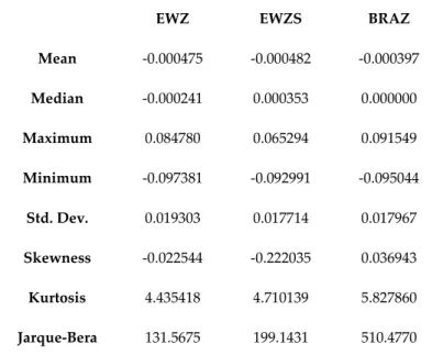
Following the existing literature on the subject, the daily return of each ETF is calculated as the difference of two consecutive natural logarithms. The summary statistics are reported in Table 1. As expected, the fact of analyzing a downward trend sample leads us to observe negative returns in all three ETFs. Those returns are asymmetric as indicated by a non-zero skewness and leptokurtic. Finally, the returns are non-normal with significant Jarque-Bera statistics.
Table 1: Descriptive statistics of daily returns of each ETF
EWZ EWZS BRAZ
Mean -0.000475 -0.000482 -0.000397 Median -0.000241 0.000353 0.000000 Maximum 0.084780 0.065294 0.091549 Minimum -0.097381 -0.092991 -0.095044 Std. Dev. 0.019303 0.017714 0.017967 Skewness -0.022544 -0.222035 0.036943 Kurtosis 4.435418 4.710139 5.827860 Jarque-Bera 131.5675 199.1431 510.4770 This table presents descriptive statistics for the daily return series of each ETF for the sample period from October 1, 2010 to October 31, 2016. Skewness and Kurtosis refer to the series skewness and kurtosis coefficients. The Jarque–Bera statistic tests the normality of the series. This statistic has an asymptotic χ2 distribution under the
nor-mal distribution hypothesis.
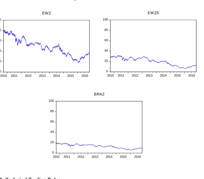
From the examination of plots of the prices of each ETF, which are displayed in Figure 1, we observe a higher volatility of the EWZ ETF when compared with the other two ETFs due to its sharp reversals during the sample analyzed. That fact could lead investors to favor investments in EWZS and BRAZ ETFs.
Figure 1: Performance of ETFs 0 20 40 60 80 100 2010 2011 2012 2013 2014 2015 2016 EWZ 0 20 40 60 80 100 2010 2011 2012 2013 2014 2015 2016 EWZS 0 20 40 60 80 100 2010 2011 2012 2013 2014 2015 2016 BRAZ
3.2 Technical Trading Rules
Initially, we employ two families of popular trading rules that have been extensively applied in the previous literature: moving average and support and resistance or trading range break.
A simple moving average is an average of observations over several consecutive time peri-ods. An n-day moving average is calculated by adding the prices of the last n days and dividing the total by n. Once calculated, a new price is added and the oldest price is dropped.
Under a simple moving average rule a buy signal is generated when a price breaks above the moving average and a sell signal is generated by a price break below the moving average. Another option is to use a short and a long period moving average. In that case a buy signal is generated when the short period moving average rises above the long period one, while a sell signal is gener-ated when the short period moving average falls below the long period one.
Following those tips, the first rule, R1, is based on the simple moving average breaks above or below the prices. Therefore, this basic trading rule opens a long (short) position when the price at time t, Pt, breaks above (below) the simple moving average of k days. Positions are maintained in this strategy, as well as in the rest, till the end of each signal.
Short Go then P k 1 P If Long Go then P k 1 P If R1 1 k 0 j t j t 1 k 0 j t j t (1)A range of 10 to 200 (by steps of 1) is specified for k. That range, which is also used by Ger-ritsen (2016), requires that 191 tests be performed in this strategy.
Rule 2, R2, generates trading signals based on the crosses of a short moving average (s) and a long moving average (l). In this case a long (short) position is opened when the shorter moving average moves above (below) the longer moving average.
Short
Go
then
P
l
1
P
s
1
If
Long
Go
then
P
l
1
P
s
1
If
R2
1 l 0 j t j 1 s 0 j t j 1 l 0 j t j 1 s 0 j t j (2)We set s and l with ranges of 10 to 70 and 70 to 200 (by steps of 10) respectively. All the combinations of these parameters are used. Therefore, a total of 1647 tests are performed.
The second family is the Trading Range Break (TRB) or support and resistance rule which generates a buy (sell) signal when the price rises above (falls below) the resistance (support) level, which refers to the highest (lowest) over the k most recent days. That technique has also widely been used in the previous empirical evidence with different results; see Bessembinder and Chan (1995), Hudson et al. (1996), Shynkevich (2012), Yu et al. (2013) and Fang et al. (2014) among others.
Following this TRB rule we propose a third proposal, R3, where the trader opens a long (short) position when the price rises above (falls below) the local maximum (minimum) of k days.
trading Not Otherwise Short Go then P min P If Long Go then P max P If R3 t j k , 1, j t j t k , 1, j t (3)
A range of 10 to 200 (by steps of 1) is specified for k. Therefore, 191 tests are performed in this strategy.
Besides those rules, which have been commonly used in the previous empirical evidence with dissimilar results, most of those unprofitable for investors, we propose to employ another one, which is referred to the momentum indicator.
Following Hsu and Kuan (2005), Schulmeister (2009) and Kuang et al. (2014) among others, we use the Rate of Change (ROC), which is defined as the current price of an asset divided by the price at time t-k. k t t t P P OC R (4)
In order to avoid misunderstandings, it is also important to point out that this paper does not follow the line of Fraser and Page (2000), Hoffman (2012), Moskowitz et al. (2012), Tse (2015), Marshall et al. (2017), and Narayan et al. (2017) among others, who also analyze the time series mo-mentum effect. Both terms are related but, as pointed out by Moskowitz et al. (2012), the time series momentum effect matches the predictions of different theories while the momentum technical indi-cator focuses purely on the security’s own past return. It must be pointed out that the main differ-ence between momentum indicator and time series momentum investing is that the former is an arithmetic calculation technical traders use to identify the speed of a trend while the latter entails buying a security just because it is going up without measuring the rate of change or considering
any other factors. That way of investing gives people the wrong idea about what the word momentum
means to real technical traders.
As well as Hsu and Kuan (2005), Schulmeister (2009), and Kuang et al. (2014), we use the basic trading rule of buying when The Rate of Change (ROC) turns from below the one line to above (or when it turns from negative into positive when calculated as a percentage) and selling when it turns from above the one line (or zero line) to below. Consequently, rule 4, R4, proposes to enter long (short) when the ROC on day t turns from below (above) the reference line of one to above (below). Short Go then 1 OC R If Long Go then 1 OC R If R4 t t (5)
Once again, a range of 10 to 200 (by steps of 1) is specified for k which leads to consider 191 tests following this strategy.
Therefore in our empirical work, we examine a total of 2220 trading rules, 191 variants for rules 1, 3 and 4 (573 in total) plus 1647 tests performed for the second rule.
3.3 Data snooping and robustness tests
The evaluation of TTRs is based on two performance measurements. The first one is the mean excess return over the buy-and-hold benchmark. The second one is the Sharpe ratio, which measures the average excess return per unit total risk. Following Urquhart et al. (2015), our initial strategy is that in which the investor assumes a buy position when a buy signal is generated and holds it until a sell signal is generated. Upon that sell signal, the investor sells and stays out of the market until the next buy signal. We label that strategy as “long”.
For robustness purposes, we examine a second strategy where short positions are allowed when a sell signal is generated. We refer to that strategy as “long and short”.
Once evaluated the performance of the TTRs, it is necessary to assess their effectiveness in the presence of data snooping bias. In other words, we test the null hypothesis that the better per-formance of a trading rule against the benchmark is not just based on luck.
For that reason, we let fk,t(k=1, …, M) be the period t return from the k-th trading rule, out of an universe of M rules, relative to the benchmark. The performance statistic for trading rule k is defined as follows:
T R t k,t k f n 1 f (6)where n=T-R+1, R is the first day in the sample when a trading signal is generated for each trading rule in the set and T is the number of periods in the sample. Based on that measurement, the Reality Check proposed by White (2000) tests the null that the performance of the best trading rule from the universe of M rules is no better than the benchmark strategy.
0 f : H k M , , 1 k o
max
(7)In order to test the null, we adopt the stationary bootstrap method of Politis and Romano (1994). Following that procedure, each time series of relative returns fk,t is resampled with replace-ment B times to generate synthetic data denoted as fk*,t,b. For each rule the procedure yields B means, therefore:
b 1, ,B
f n 1 f T R t * b , t , k * b , k
(8)The test then involves comparing the following two statistics to obtain the p-value:
k M , , 1 k f n Vmax
(9) k * b , k M , , 1 k * f f n Vmax
(10)We accumulate B values of V* and estimate the p-value as:
V V
P * (11)
If the p-value is smaller than a certain significance level, we consider that the null hypothesis is rejected. That rejection leads to the conclusion that the best TTR outperforms the benchmark, tak-ing into account the data snooptak-ing effects.
White (2000) chooses the least favorable configuration (LFC) to obtain the null distribution which it is convenient but also renders this test relatively conservative. Additionally, another prob-lem of the Reality Check test is that its statistic is not studentized, which means that it avoids a comparison of trading rules performances measured in different units of standard deviation.
In order to solve those problems Hansen (2005) proposes the Superior Predictive Ability (SPA) test, which is based in the following statistic:
ˆ ,0 f n T k k M , , 1 kmax (12)
where ˆk represents the estimator of the standard deviation of nfk.
In order to proceed with the SPA tests and evaluate the p-value, we need to estimate the statistics for each bootstrap sample:
ˆ ,0 Z n T k k M , , 1 k * max (13) where
n 1 t k,t k Z n 1 Z (14)
nf ˆ 2lnln n
1 f f Zk,t k*,b k kk (15)where 1(·) is an indicator function taking on the value of 1 if the expression in parentheses is true and 0 otherwise.
One bootstrap sample will give one T*. We then re-estimate T* until there are B values of it. The bootstrap p-value could then be given as:
B 1 i * i B T T 1 p (16)Finally, Hansen (2005) recommends calculating the lower and upper bounds for the con-sistent p-values as:
f ,0 b 1, ,B max f ZLk k*,b k (17) B , , 1 b f f ZUk k*,b k (18) 4 EMPIRICAL RESULTSTable 2 shows the performances of the best technical trading rules according to both the mean excess returns (Panels A and C) and the Sharpe ratio (Panels B and D), for both strategies.
Trading strategy: Long Panel A: Mean Return Criterion ETF Best trading rule Mean excess
re-turn Pnom, W Pnom, H
p-value (RC) p-value (SPAl) p-value (SPAc) p-value (SPAu) EWZ R4 (k=50) 0.170 0.054 0.042 0.092 0.086 0.081 0.081 EWZS R4 (k=37) 0.236*** 0.013 0.008 0.029 0.014 0.019 0.029 BRAZ R4 (k=31) 0.152 0.042 0.046 0.096 0.104 0.104 0.087
Panel B: Sharpe Ratio Criterion ETF Best trading rule Sharpe ratio Pnom, W Pnom, H p-value
(RC) p-value (SPAl) p-value (SPAc) p-value (SPAu) EWZ R4 (k=50) 0.681 0.015 0.026 0.065 0.079 0.081 0.086 EWZS R1 (k=21) 0.654*** 0.005 0.004 0.007 0.005 0.004 0.005 BRAZ R4 (k=31) 0.663 0.027 0.032 0.086 0.089 0.098 0.083
Trading strategy: Long-Short Panel C: Mean Return Criterion ETF Best trading rule Mean excess
re-turn Pnom, W Pnom, H
p-value (RC) p-value (SPAl) p-value (SPAc) p-value (SPAu) EWZ R4 (k=50) 0.287 0.066 0.057 0.106 0.090 0.104 0.103 EWZS R4 (k=37) 0.422*** 0.008 0.008 0.018 0.021 0.020 0.019 BRAZ R3 (k=36) 0.267 0.043 0.049 0.109 0.115 0.126 0.109
Panel D: Sharpe Ratio Criterion ETF Best trading rule Sharpe ratio Pnom, W Pnom, H p-value
(RC) p-value (SPAl) p-value (SPAc) p-value (SPAu) EWZ R1 (k=108) 0.666 0.008 0.007 0.011 0.012 0.013 0.009 EWZS R4 (k=37) 1.068*** 0.006 0.001 0.014 0.012 0.015 0.023 BRAZ R3 (k=36) 0.652 0.041 0.044 0.119 0.110 0.119 0.110 This table reports the performance of the best trading rule from the universe of 2220 trading rules for each ETF under two alternative criteria. The number of days in a moving average, support and resistance range and Rate of Change is denoted by k. The mean excess returns and Sharpe ratio are both annualized. Pnom, W and Pnom, H denote White’s Reality Check and Hansen’s Superior Predictive Ability nominal
p-values which are calculated by applying each methodology to the best trading rule only, thereby ignoring the effect of data snooping. P-value RC denotes White’s Reality Check p-value while p-value SPAl,
SPAc and SPAu denote Hansen’s Superior Predictive Ability lower, consistent, and upper p-values, respectively. Those p-values are computed by applying each methodology to the universe of 2220 trading
consistent and upper) from the SPA test are provided after adjusting for data snooping bias. Fur-thermore, following Sullivan et al. (1999), Shynkevich (2012), Kuang et al. (2014) and Yamamoto (2016) nominal p-values are also reported. They are obtained by applying the Reality Check and the SPA tests to the best rules ignoring the data snooping bias. They are less reliable but are shown for illustrative purposes.
From a preliminary analysis, we observe that in accordance with the results obtained by Hsu
et al. (2010) and Tse (2015), there is no possibility of developing a technical trading rule that outper-forms the buy-and-hold benchmark when those technical trading rules are applied to the iShares MSCI Brazil Capped ETF (EWZ), which tracks the MSCI Brazil 25/50 Index, i.e. the largest companies of the Brazilian stock market. We find that the mean excess returns and Sharpe ratios are not statis-tically significant for any of the strategies. The p-values from the Reality Check and SPA tests show that there are profitable rules in theory for most of the cases. However, we consider that the fact of not rejecting the null that both the mean excess return and Sharpe ratio from the best trading rule is not different from zero is enough evidence of the weakness of the technical trading rules for this ETF.
The results for the Global X Brazil Mid Cap ETF (BRAZ) which tap the mid cap market of the Brazilian stock market by tracking the Solactive Brazil Mid Cap Index are similar to those found for the larger companies. Once again both performance measurements are not statistically significant and the null that the benchmark is not inferior to any of the alternative trading rules is not rejected in many cases.
The most interesting results are obtained from developing the proposed rules over the iShares MSCI Brazil Small-Cap ETF (EWZS), which focuses on small companies of the Brazilian stock market by tracking the MSCI Brazil Small Cap Index. We find that both mean excess return and Sharpe ratios provide statistically significant positive values at the 1% level for both strategies. Additionally, in all cases the best rule, which is based on the Rate-of-Change indicator (R4), shows a significant evidence of superior predictive ability because the null hypothesis that the benchmark (buy-and-hold strategy) is not inferior to any of the alternative trading rules is overwhelmingly re-jected at 5% level of significance.
Those findings suggest that investors must focus the development of technical trading rules on smaller companies of the Brazilian stock market, rather than on larger ones. This makes sense, considering that previous empirical evidence has proven that smaller companies have got higher performances than larger ones for the same period, see Van Dijk (2011), Cakici et al. (2013) and Israel and Moskowitz (2013), among others.
However, considering that the previous results can be conditioned by the existence of trans-action costs. Sanvicente (2012) indicates that average transtrans-action costs in the Brazilian stock market fell from 0.0295% in 1999 to 0.0122% in 2009. These values are consistent with the current fee sched-ule reported by BM&F Bovespai. However, in order to give more strength to our findings we re-estimate the previous rules and strategies taking into account a one way transaction cost of 10 basis points (which means a 0.20% roundtrip transaction cost). This value is consistent with the maximum costs shown by Sanvicente (2012) for the Brazilian stock market and follows the same procedure used by Lee et al. (2001), Shynkevich (2012) and Kuang et al. (2014) among others. Results are re-ported in Table 3.
In accordance with the results obtained by Milionis and Papanagiotou (2009) and Kuang et al. (2014) among others, the performance of all rules decreases. Nevertheless, it is interesting to point out that the proposed active rule 4, which is based on following the Rate-of-Change indicator, main-tains higher performances than those obtained with the passive strategy when applied on the ETF that tracks the smaller companies of the Brazilian stock market. We can observe, once again, that the
Based on the results shown in Table 3, an investor who opts for investing on small companies of the Brazilian stock market by means of the EWZS ETF would gain an annualized mean excess return of 22.7% over the passive buy-and-hold strategy by using our proposed long strategy (which does not enable for short positions) over a 37-day rate of change. That gain grows from 22.7% to 40.6% if our proposed long-and-short strategy (which enables for short positions) is chosen, also over a 37-day rate of change. In both cases, a statistically significant Sharpe ratio close to 1 is ob-tained, which is commonly considered acceptable to good by investors.
Trading strategy: Long Panel A: Mean Return Criterion ETF Best
trading rule
Mean
ex-cess return Pnom, W Pnom, H
p-value (RC) p-value (SPAl) p-value (SPAc) p-value (SPAu) EWZ R1 (k=160) 0.166 0.049 0.060 0.115 0.109 0.114 0.099 EWZS R4 (k=37) 0.227*** 0.008 0.007 0.030 0.023 0.029 0.018 BRAZ R3 (k=36) 0.147 0.048 0.051 0.106 0.102 0.110 0.114
Panel B: Sharpe Ratio Criterion ETF Best
trading rule
Sharpe
ratio Pnom, W Pnom, H
p-value (RC) p-value (SPAl) p-value (SPAc) p-value (SPAu) EWZ R4 (k=50) 0.632 0.032 0.030 0.107 0.077 0.099 0.093 EWZS R4 (k=37) 0.991*** 0.000 0.002 0.008 0.008 0.007 0.006 BRAZ R3 (k=36) 0.624 0.027 0.031 0.104 0.114 0.102 0.112
Trading strategy: Long-Short Panel C: Mean Return Criterion ETF Best
trading rule
Mean
ex-cess return Pnom, W Pnom, H
p-value (RC) p-value (SPAl) p-value (SPAc) p-value (SPAu) EWZ R3 (k=46) 0.277 0.048 0.55 0.106 0.112 0.089 0.111 EWZS R4 (k=37) 0.406*** 0.008 0.010 0.021 0.025 0.027 0.027 BRAZ R3 (k=36) 0.260 0.052 0.049 0.093 0.113 0.123 0.127
Panel D: Sharpe Ratio Criterion ETF Best
trading rule
Sharpe
ratio Pnom, W Pnom, H
p-value (RC) p-value (SPAl) p-value (SPAc) p-value (SPAu) EWZ R1 (k=108) 0.639 0.036 0.040 0.104 0.096 0.103 0.092 EWZS R4 (k=37) 1.025*** 0.008 0.007 0.015 0.018 0.015 0.020 BRAZ R3 (k=37) 0636 0.042 0.050 0.108 0.125 0.109 0.119 This table reports the performance of the best trading rule from the universe of 2220 trading rules for each ETF under two alternative criteria. The number of days in a moving average, support and resistance range and Rate of Change is denoted by k. The mean excess returns and Sharpe ratio are both annualized. Pnom, W and Pnom, H denote White’s Reality Check and Hansen’s Superior Predictive Ability
nominal values which are calculated by applying each methodology to the best trading rule only, thereby ignoring the effect of data snooping. P-value RC denotes White’s Reality Check value while p-value SPAl, SPAc and SPAu denote Hansen’s Superior Predictive Ability lower, consistent, and upper p-values, respectively. Those p-values are computed by applying each methodology to the universe of
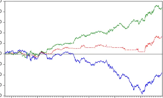
lative returns of the R4 for a 37-day time span of the EWZS for both strategies (long and long and short), and the cumulative returns of the buy-and-hold strategy (CR BH) for the same ETF. We can undoubtedly observe that the buy-and-hold strategy, which follows a clear downward trend, is sig-nificantly outperformed by both strategies.
Figure 2: Cumulative returns of the best trading rule and the benchmark (values in percentages)
The figure plots the cumulative returns of the benchmark, long strategy and long-short strategy for the rule 4 applied to EWZS
5 CONCLUSIONS
The objective of this paper has been to analyze different trading strategies for the Brazilian stock market. This analysis is focused on the comparison and combination of different active rules against the passive rule of buy-and-hold. We have improved the empirical evidence by comparing the performance of active strategies based on classical TTRs with a proposal based on the momen-tum indicator. We also analyze large, medium and small companies of the Brazilian stock market in order to provide a better vision of the investment opportunities on it, and, finally, Reality Check and Superior Predictive Ability tests were employed to account for possible data snooping bias.
From the initial results, we find that the better performances are provided by the trading rule based on the momentum indicator, specifically the Rate of Change. That rule clearly outperforms the technical trading rules based on the moving average and support and resistance. However, the most important finding is the fact that the null hypothesis that the performance of the best trading rule is worse than that of the benchmark (buy-and-hold rule) is only rejected when the rule based on the rate of change indicator is employed over the iShares MSCI Brazil Small-Cap ETF (EWZS), i.e. the ETF which tracks the small companies of the Brazilian stock market.
Those results are very interesting and shed new light on a number of important issues such as the capability of the Brazilian stock market to generate significant mean excess returns and sig-nificant positive Sharpe ratios. As a result, it has been proven that previous empirical evidence was erroneously focused on larger companies, using the iShares MSCI Brazil Capped ETF (EWZ) as the main reference of the Brazilian stock market, instead of using the iShares MSCI Brazil Small-Cap
-160 -120 -80 -40 0 40 80 120 160 200 2010 2011 2012 2013 2014 2015 2016
ETF (EWZS), which tracks the small companies. We clearly show that the latter provide much better performance results when compared with other ETFs and technical analysis trading rules are used. To summarize, we have proven the importance of using the momentum indicator as the basis for obtaining the best trading rule and that the buy-and-hold passive strategy can be clearly outper-formed. The results obtained seem to have important implications for planning investment strate-gies and understanding the world’s main stock indexes.
REFERENCES
Bessembinder, H., & Chan, K. (1995). The profitability of technical trading rules in the Asian stock markets. Pacific-Basin Finance Journal, 3, 257-284. https://doi.org/10.1016/0927-538X(95)00002-3
Brock, W., Lakonishok, J., & LeBaron, B. (1992). Simple technical trading rules and the stochastic properties of stock returns. Journal of Finance, 47, 1731-1764. doi:10.1111/j.1540-6261.1992.tb04681.x
Cacique da Costa, T., Nazário, R.T., Bergo, G., Sobreiro, V., & Kimura, H. (2015). Trading system based on the use of technical analysis: A computational experiment. Journal of Behavioral and Experimental Finance, 6, 42-55. https://doi.org/10.1016/j.jbef.2015.03.003
Cakici, N., Fabozzi, F., & Tan, S. (2013). Size, value, and momentum in emerging market stock re-turns. Emerging Markets Review, 16, 46-65. https://doi.org/10.1016/j.ememar.2013.03.001 Chang, E.J., Lima, E., & Tabak, B. (2004). Testing for predictability in emerging equity markets.
Emerging Markets Review, 5, 295-316. https://doi.org/10.1016/j.ememar.2004.03.005
Cootner, P.H. (1962). Stock prices: random vs. systematic changes. Industrial Management Review, 3, 24–45. http://www.e-m-h.org/Coot62.pdf
Fama, E., & Blume, M. (1966). Filter rules and stock market trading. Journal of Business, 39, 226-241. http://www.e-m-h.org/FaBl66.pdf
Fang, J., Qin, Y., & Jacobsen, B. (2014). Technical market indicators: An overview. Journal of Behavioral and Experimental Finance, 4, 25-56. https://doi.org/10.1016/j.jbef.2014.09.001
Fraser, E., & M. Page. (2000). Value and momentum strategies: Evidence from the Johannesburg Stock Exchange. Investment Analysts Journal, 29, 25-35. http://dx.doi.org/10.1080/10293523.2000.11082404
Gerritsen, D.F. (2016). Are chartists artists? The determinants and profitability of recommendations based on technical analysis, International Review of Financial Analysis, 47, 179-196. https://doi.org/10.1016/j.irfa.2016.06.008
Gunasekarage, A., & Power, D.M. (2001). The profitability of moving average trading rules in South Asian stock markets. Emerging Markets Review, 2, 17-33. https://doi.org/10.1016/S1566-0141(00)00017-0
Hansen, P.R. (2005). A test for superior predictive ability. Journal of Business and Economic Statistics,
23, 365-380. http://dx.doi.org/10.1198/073500105000000063
Hatgioannides, J., & Mesomeris, S. (2007). On the returns generating process and the profitability of trading rules in emerging capital markets. Journal of International Money and Finance, 26, 948-973. https://doi.org/10.1016/j.jimonfin.2007.05.005
Hoffman, A.J. (2012). Stock return anomalies: Evidence from the Johannesburg Stock Exchange. In-vestment Analysts Journal, 41, 21-41. http://dx.doi.org/10.1080/10293523.2012.11082542 Hsu, P.H., Hsu, Y.C., & Kuan, C.M. (2010). Testing the predictive ability of technical analysis using
a new stepwise test without data snooping bias. Journal of Empirical Finance, 17, 471-484. https://doi.org/10.1016/j.jempfin.2010.01.001
Hsu, P. H., & Kuan, C.M. (2005). Reexamining the profitability of technical analysis with data snoop-ing checks. Journal of Financial Econometrics, 3, 606-628. https://doi.org/10.1093/jjfinec/nbi026 Hudson, R., Dempsey, M., & Keasey, K. (1996). A note on the weak form efficiency of capital mar-kets: the application of simple technical trading rules to UK stock prices - 1935 to 1994, Journal of Banking & Finance, 20, 1121-1132. https://doi.org/10.1016/0378-4266(95)00043-7
Israel, R., & Moskowitz, T. (2013). The role of shorting, firm size, and time on market anomalies.
Journal of Financial Economics, 108, 275-301. http://dx.doi.org/10.1016/j.jfineco.2012.11.005 Jegadeesh, N., & Titman, S. (1993). Returns to buying winners and selling losers: implications for
stock market efficiency. Journal of Finance, 48, 699-720. doi: 10.1111/j.1540-6261.1993.tb04702.x Jegadeesh, N., & Titman, S. (2001). Profitability of momentum strategies: an evaluation of alternative
explanations. Journal of Finance, 56, 699-720. doi: 10.1111/0022-1082.00342
Kuang, P., Schröder, M., & Wang, Q. (2014). Illusory profitability of technical analysis in emerging foreign exchange markets. International Journal of Forecasting, 30, 192-205. https://doi.org/10.1016/j.ijforecast.2013.07.015
Kwon, K.Y., & Kish, R.J. (2002). A comparative study of technical trading strategies and return pre-dictability: an extension of Brock, Lakonishok, and LeBaron (1992) using NYSE and NASDAQ indices. The Quaterly Review of Economics and Finance, 42, 611-631. https://doi.org/10.1016/S1062-9769(01)00089-8
Lee, C.I., Gleason, K.C., & Mathur, I. (2001). Trading rule profits in Latin American currency spot rates. International Review of Financial Analysis, 10, 135–156. https://doi.org/10.1016/S1057-5219(01)00042-4
Lo, A. (2004). The Adaptive Market Hypothesis: Market efficiency from an evolutionary perspective.
Marshall, B.R., Nguyen, N.H., & Visaltanachoti, N. (2017). Time series momentum and moving av-erage trading rules. Quantitative Finance, 17 (3), 405-421. http://dx.doi.org/10.1080/14697688.2016.1205209
Milionis, A.E., & Papanagiotou, E. (2009). A study of the predictive performance of the moving av-erage trading rule as applied to NYSE, the Athens Stock Exchange and the Vienna Stock Ex-change: sensitivity analysis and implications for weak-form market efficiency testing. Applied Financial Economics, 19 (14), 1171-1186. http://dx.doi.org/10.1080/09603100802375519
Mitra, S.K., (2011). How rewarding is technical analysis in the Indian stock market? Quantitative Fi-nance, 11(2), 287-297. http://dx.doi.org/10.1080/14697680903493581.
Moskowitz, T.J., Ooi, Y.H., & Pedersen, L.H. (2012). Time series momentum. Journal of Financial Eco-nomics, 104, 228-250. https://doi.org/10.1016/j.jfineco.2011.11.003
Narayan, P.K., Ahmed, H.A., Sharma, S.S., & Prabheesh, K.P. (2014). How profitable is the Indian stock market? Pacific Basin Finance Journal, 30, 44-61. https://doi.org/10.1016/j.pacfin.2014.07.001
Narayan, P.K., Phan, D., & Bannigidadmath, D. (2017). Is the profitability of Indian stocks compen-sation for risks? Emerging Markets Review, Forthcoming. https://doi.org/10.1016/j.eme-mar.2017.02.001
Ni, Y., Liao, Y.C., & Huang, P. (2015). MA trading rules, herding behaviors, and stock market over-reaction. International Review of Economics and Finance, 39, 253-265. https://doi.org/10.1016/j.iref.2015.04.009
Parisi, F., & Vasquez, A. (2000). Simple technical trading rules of stock returns: evidence from 1987 to 1998 in Chile. Emerging Markets Review, 1, 152-164. https://doi.org/10.1016/S1566-0141(00)00006-6
Politis, D.N., & Romano, J.P. (1994). The stationary bootstrap. Journal of the American Statistical Asso-ciation, 89, 1303-1313. http://www.jstor.org/stable/2290993
Ratner, M., & Leal, R.P.C. (1999). Tests of technical trading strategies in the emerging equity markets of Latin America and Asia. Journal of Banking & Finance, 23, 1887-1905. https://doi.org/10.1016/S0378-4266(99)00042-4
Sanvicente, A.Z. (2012). Determinants of transaction costs in the Brazilian stock market. Revista
Brasileira de Finanças, 10 (2), 179-196.
http://bibliotecadigital.fgv.br/ojs/index.php/rbfin/article/download/3536/2686
Schulmeister, S. (2009). Profitability of technical stock trading: has it moved from daily to intraday data? Review of Financial Economics, 18 (4), 190-201. https://doi.org/10.1016/j.rfe.2008.10.001 Shynkevich, A. (2012). Performance of technical analysis in growth and small cap segments of the
US equity market. Journal of Banking & Finance, 36, 193-208. https://doi.org/10.1016/j.jbankfin.2011.07.001
Sobreiro, V.A., Cacique da Costa, T., Nazário, R.T., Lima e Silva, J., Moreira, E.A., Lima Filho, M., Kimura, H., & Zambrano, J.C. (2016). The profitability of moving average trading rules in BRICS and emerging stock markets. North American Journal of Economics and Finance, 38, 86-101. https://doi.org/10.1016/j.najef.2016.08.003
Sullivan, R., Timmermann, A., & White, H. (1999). Data-snooping, technical trading rule perfor-mance, and the bootstrap. Journal of Finance, 54, 1647-1691. doi: 10.1111/0022-1082.00163 Sweeney, R. J. (1988). Some new filter rule tests: Methods and results. Journal of Financial and
Quan-titative Analysis, 23, 285-300. https://doi.org/10.2307/2331068
Taylor, N. (2014). The rise and fall of technical trading rule success. Journal of Banking & Finance, 40, 286-302. https://doi.org/10.1016/j.jbankfin.2013.12.004
Tse, Y. (2015). Momentum strategies with stock index exchange-traded funds. North American Journal of Economics and Finance, 22, 134-148. https://doi.org/10.1016/j.najef.2015.04.003
Ülkü, N. & Prodan, E. (2013). Drivers of technical trend-following rules’ profitability in world stock
markets. International Review of Financial Analysis, 30, 214-229. https://doi.org/10.1016/j.irfa.2013.08.005
Urquhart, A., Gebka, B., & Hudson, R. (2015). How exactly do markets adapt? Evidence from the moving average rule in three developed markets. Journal of International Financial Markets, Institutions & Money, 38, 127-147. https://doi.org/10.1016/j.intfin.2015.05.019
Van Dijk, M. (2011). Is size dead? A review of the size effect in equity returns. Journal of Banking and Finance, 35, 3263-3274. https://doi.org/10.1016/j.jbankfin.2011.05.009
White, H. (2000). A reality check for data snooping. Econometrica, 68, 1097-1126. doi: 10.1111/1468-0262.00152
Yamamoto, R. (2016). Trading profitability from learning and adaptation on the Tokyo Stock Ex-change. Quantitative Finance, 16(6), 969-996. http://dx.doi.org/10.1080/14697688.2015.1091941. Yu, H., Nartea, G.V., Gan, C., & Yao, L.J. (2013). Predictive ability and profitability of simple
tech-nical trading rules: Recent evidence from Southeast Asian stock markets. International Review of Economics and Finance, 25, 356-371. https://doi.org/10.1016/j.iref.2012.07.016
i http://www.bmfbovespa.com.br/en_us/services/fee-schedules.