Nonparametric estimation of mean and dispersion
functions in extended generalized linear models
I. Gijbels1,3, I. Prosdocimi1,3 and G. Claeskens2,3
1 Department of Mathematics, Katholieke Universiteit Leuven
2 Operations Research and Business Statistics, Katholieke Universiteit Leuven 3 Leuven Statistics Research Center (LStat), Katholieke Universiteit Leuven, Belgium.
Abstract
We study joint nonparametric estimators of the mean and the dispersion function in extended double exponential family models. The starting point is the exponen-tial family and the generalized linear models setting. The extended models allow for both overdispersion and underdispersion, or even a combination of both. We simultaneously estimate the dispersion function and the mean function by using P-splines with a difference type of penalty to avoid overfitting. Special attention is given to the smoothing parameter selection as well as to implementation issues. The performance of the method is investigated via simulations. A comparison with other available methods is made. We provide applications to several sets of data, including continuous data, counts and proportions.
Keywords and phrases: Double exponential family; Extended quasi-likelihood;
Non-parametric regression; Overdispersion; P-splines; Variance estimation; Underdispersion.
1
Introduction
The aim of this work is to provide tools to nonparametrically estimate mean and dispersion functions. In a specific generalized linear model a fixed relationship exists between the mean and the variance. For example, for the Poisson distribution the mean is equal to the variance. Real data often show a larger variability than what we would expect from the theoretical model. This phenomenon is referred to as overdispersion. The opposite situation of less variability occurs less frequently and is called underdispersion. Our approach can deal with both overdispersed and underdispersed data, coming from different distributions originating from the exponential family. As such it is a unified approach not requesting special models for overdispersion such as a beta-binomial for proportion data or a negative binomial for count data. We start from a double exponential family (Efron
(1986)), and model both the mean and the dispersion function as smooth functions of the covariate through P-splines (Eilers and Marx (1996)). The flexible modeling even allows for dispersion functions that might reveal underdispersion in one region of the covariate-domain and overdispersion in other regions.
Hinde and Dem´etrio (1998) give an overview of estimation methods for overdispersed data. Parametric models for the dispersion as a function of one or more covariates include extended quasi-likelihood (Nelder and Pregibon (1987); McCullagh and Nelder (1989)), the double exponential regression models (see Efron (1986); Galfand and Dalal (1990); Deyet al. (1997)), and the pseudo-likelihood approach proposed by Davidian and Carroll (1987), among others. All these approaches have their advantages and disadvantages. See for example Nelder and Lee (1992), Lee and Nelder (2000) and Davidian and Carroll (1988) for a comparison of methods. They all share the common feature of being based on parametric modeling. Some work has been done on flexible modeling of overdisper-sion, see for example Aerts and Claeskens (1997), Chapter 14 in Ruppert et al. (2003) and Nott (2006). The latter uses a mixed model representation of splines in the double exponential family framework to get to a Bayesian estimation of both the mean and the variance function. Rigby and Stasinopoulos (2005) propose generalized additive models for location, scale and shape, in which they nonparametrically estimate different parame-ters of a distribution using a mixed model approach and concepts of hierarchical modeling. Earlier references on hierarchical modeling include Lee and Nelder (1996, 2001).
Estimating the unknown variance/dispersion is of interest to improve the estimation of the mean and can, in different contexts, be an issue of importance on its own. See for example Carroll and Ruppert (1988), for the importance and utility of estimating variance functions in the linear regression context.
In Section 2 we briefly discuss the framework for the estimation procedure. The nonparametric procedure for estimating mean and dispersion function using penalized regression techniques is presented in Section 3 including a discussion on practical choices of smoothing parameters. A simulation study investigating the performance of the esti-mation procedure is provided in Section 4, which also includes a comparison with other existing methods. Section 5 contains illustrations with real data examples. In Section 6 we provide some further discussions.
2
The double exponential family for joint modeling
of mean and dispersion function
Efron (1986) introduced the double exponential family of distributions. This is a general-ization of the exponential family in which an extra parameter controlling the variance is added.
In a one-parameter exponential family, denoted by (Y|X = x) ∼ EF(b(θ(x)), φ), the conditional density of the response variable Y given the covariate X =x, is of the form
eY(y;θ(x), φ) = exp yθ(x)−b(θ(x)) φ +c(y, φ) . (2.1)
Here b(·) and c(·) are known functions, identifying specific distributions (including the normal, the Poisson and the binomial distribution). The natural location parameter is
θ and φ is the scale parameter. The moments for the exponential family correspond to
µ(x) =E[Y|X =x] =b′(θ(x)) and Var[Y|X =x] =φb′′(θ(x)). It is assumed throughout
that (b′)−1 exists and that b′′(·)6= 0.
The double exponential family
For simplicity of presentation we introduce this family in a non-regression setup, as in Efron (1986). The density of a variable Y coming from the double exponential family
Y ∼DEF(b(θ), φ, γ)) is ˜ fY(y;θ, φ, γ) = c(θ, γ)γ− 1 2eY(y;θ, φ) 1 γe Y(y;θS, φ)1 −γ1 , (2.2)
where θS is the choice of θ corresponding to the saturated one-parameter exponential
model Y ∼ EF(b(θ), φ), namely θS = (b′)−1(y), which maximizes eY(y;θ, φ) over all
possible values ofθ andc(θ, γ) is a normalizing constant, such thatR∞
−∞f˜Y(y;θ, φ, γ)dy =
1. Efron (1986) shows that the constantc(θ, γ) in (2.2) can be (first order) approximated by 1, so that an approximation of (2.2) is fY(y;θ, φ, γ) = γ− 1 2e Y(y;θ, φ) 1 γe Y(y;θS, φ)1 −1γ . (2.3)
This approximation works quite well overall, but might be poorer for extremely overdis-persed and underdisoverdis-persed cases with a small mean. For a detailed study on the use of the unnormalized form (2.3) of the density for inference see Lee and Nelder (2000). As suggested and motivated in Efron (1986) we use this approximated formulation of the
double exponential family, which leads to a convenient implementation of the inference procedure.
It can be shown that forY ∼DEF(b(θ), φ, γ) we approximately have thatE(Y) =µ=
b′(θ) and Var[Y] =γφb′′(θ) (see Formula (3.21) in Efron (1986)), and clearly whenγ = 1
the double exponential family reduces to Y ∼ EF(b(θ), φ) in (2.1), while for γ > 1(< 1) we have overdispersion (underdispersion). In other words, γ is the parameter describing the dispersion.
For the one-parameter exponential family (2.1), the deviance is defined as
d(y, θ) = 2[log(eY(y;θS, φ))−log(eY(y;θ, φ))] = 2 yθS−b(θS) φ − yθ−b(θ) φ . (2.4)
Therefore we can rewrite (2.3) as
fY(y;θ, φ, γ) =γ− 1 2 exp 1 2d(y, θ) −1γ eY(y;θS, φ).
This is helpful in getting an elegant expression of the log-likelihood when considering the regression case.
When using double exponential families in a regression context one is interested in studying how the expected value and the dispersion of Y depend on a covariate X. It is assumed that (Y|X = x) ∼ DEF(b(θ(x)), φ, γ(x)), with φ a known constant, not dependent on X. Similarly as in the one-parameter exponential family we introduce a link function g and consider η(x) = g(µ(x)), with µ(x) = E[Y|X = x]. In parametric models we might fit a linear function of the covariate,η(x) =β0+β1x, withβ = (β0 , β1)T
the vector of unknown parameters. Here the superscript T denotes the transposed of a vector (or matrix). For the canonical linkη(x) =g(b′(θ(x))) =θ(x). From now on, unless
otherwise mentioned, we will always use canonical link functions.
When working within the double exponential family we also use a regression model for the dispersion function. In a parametric (linear) setting this would mean that we model a transformation of the dispersion function as a linear combination of the covariate:
γ(x) = h(ξ(x)), ξ(x) = δ0+δ1x, with δ = (δ0 , δ1)T the vector of unknown parameters.
Note that the functionh(·) needs to be chosen with care since a dispersion function should always be nonnegative (h≥0). In addition we assume that his such that h−1 exists and
h′(·)6= 0.
Throughout the remainder of this work we model the mean and the dispersion function in a double exponential family framework. Note that such a direct modeling of the
dispersion function, can handle both overdispersed and underdispersed data or even data where the appearance of overdispersion or underdispersion depends on the range of values of the covariate. The double exponential family provides a unified framework for different types of data (counts, proportions, etc.), where we can directly model the dispersion function γ(x) that can take values either larger or smaller than 1.
3
Nonparametric estimation of mean and dispersion
3.1
Estimation procedure
The goal of this work is to obtain nonparametric estimators for both the mean and the dispersion function combining the parametric approach of the double exponential family where (Y|X = x) ∼ DEF(b(θ(x)), φ, γ(x)), as discussed in Section 2, with the nonparametric P-splines technique of Eilers and Marx (1996).
Via η(x) =g(µ(x)) and ξ(x) = h−1(γ(x)) we model each of these functions as a linear
combination of B-spline basis functions (possible different sets for each) and use difference type of penalties to prevent overfitting. For the mean function, for a given set of knots
{κ1, . . . , κkµ}, B-spline basis functions of degree pµ are composed of polynomial pieces
of degree pµ, joined together in an appropriate way at each knot κj. This results into
a B-spline basis of dimension Kµ =pµ+ 1 +kµ, denoted by Bµ,1(·), Bµ,2(·), . . . Bµ,Kµ(·).
For details, see de Boor (2001). The unknown function η(·) is then modeled as η(x) =
PKµ
j=1αµ,jBµ,j(x) =BTµ(x)αµ where we denote Bµ(x) = (Bµ,1(x), . . . , Bµ,Kµ(x))
T, a
vec-tor of dimensionKµ×1, andαµ= (αµ,1, . . . , αµ,Kµ)
T, the unknown vector of spline
coeffi-cients for the mean function. Similarly, the dispersion functionγ(·) is modeled in a flexible way via a set of knots{ν1, . . . , νkγ}and B-splines of degreepγ, leading toξ(x) = B
T
γ(x)αγ,
where Bγ(x) has dimension Kγ×1 withKγ =pγ+ 1 +kγ, and αγ = (αγ,1, . . . , αγ,Kγ)
T.
Large values of Kµ and Kγ might lead to overfitting. This is avoided by introducing
penalty terms on the spline coefficients in the log-likelihood function. P-splines regression uses penalties based on higher order differences of the coefficients. For the mean estimation this leads to a penalty term PKµ
j=m+1(∆mαµ,j)2, where m is the order of the difference
operator: ∆αµ,j =αµ,j −αµ,j−1, ∆2αµ,j = ∆∆αµ,j =αµ,j−2αµ,j−1+αµ,j−2 and so on.
We consider relatively large numbers of knots Kµ and Kγ, which cover the range of
observed values ofX in the sample (x,y) from (X, Y). Based on the two sets of B-spline basis functions and the observed sample, we then define the matrix Bµ of dimension
n×Kµ, with i-th rowBTµ,i =Bµ(xi) = (Bµ,1(xi), . . . , Bµ,Kµ(xi)). In a similar manner the
matrix Bγ of dimension n×Kγ is obtained.
Maximum penalized likelihood inference for µ(x) andγ(x) follows from maximization with respect to αµ and αγ of the penalized log-likelihood
l(αµ,αγ;x,y, λµ, λγ) = n X i=1 ( log(h(BTγ,iαγ)) + 1 h(BTγ,iαγ) d(yi,BTµ,iαµ) ) −1 2λµα T µD T mDmαµ− 1 2λγα T γD T ℓDℓαγ, (3.1)
where Dm and Dℓ are the matrix representations of the m-th and ℓ-th order difference
operators, and with λµ > 0 and λγ > 0 the two smoothing parameters which penalize
respectively the estimation for the mean and the dispersion function. The choice of the parameters λµ and λγ is discussed in Section 3.2.
Maximization of (3.1) is done via an iterative two-step procedure. At each iteration i
we have the following steps:
Step (a): for a given γ(i−1)(x), choose an optimal value of λ
µ, obtain the maximizer of
(3.1) with respect to αµ denoted by ˆα(µi), and get an estimate ˆµ(i)(x) forµ(x).
Step (b): for the given ˆµ(i)(x), choose an optimal value of λγ, obtain the maximizer of
(3.1) with respect to αγ, denoted by ˆα(γi) and, get an estimate ˆγ(i)(x) forγ(x).
The iteration stops when, for a chosen small 0 < ǫ <1, we have that
1−ǫ < max 1≤j≤n BTµ,jα(µi) BTµ,jα(µi−1) , BTγ,jα(γi) BTγ,jα(γi−1) ! <1 +ǫ , where BTµ,jα(µi) (respectively BTγ,jα (i)
γ ) is the estimator for µ(xj) (respectively γ(xj)) at
the i-th iteration.
We now provide more details on the procedure.
• Step0: initial values
Some appropriate initial valuesαµ
(0) andα
γ
(0)are needed to start the iterative procedure.
In our implementation we have taken constant initial values ˆµ(0) = n−1Pn
i=1yi =y and
ˆ
γ(0) = φ
n where φn is either the known value for φ in the considered exponential model
(see Table 2.1 on page 30 of McCullagh and Nelder (1989)) or an estimator for it. For example, for the normal model φ =σ2, and in this case ˆγ(0) = (n−1)−1Pn
the empirical variance. For a Poisson model φ = 1 and for a binomial model φ = 1/N, where N is the number of trials.
With these initial values the iterative procedure is started and alternates between steps (a) and (b). Within a given iteration i two sub-steps are distinguished: the choice of an optimal smoothing parameter and maximization of (3.1). Details on the optimal choice of λµ and λγ are in Section 3.2, and more explanation on the maximization of (3.1) with
respect to αµ and αγ is provided here.
• Step(a): estimation of αµ.
To find the maximum likelihood estimator forαµ we rewrite (3.1) as a function ofαµfor a given γ(x): l(αµ;x,y, λµ) = n X i=1 1 φ γ(xi) (yi BTµ,iαµ−b(BTµ,iαµ)) −1 2λµα T µD T mDmαµ. (3.2)
As in the generalized linear models setting of Eilers and Marx (1996) this system can-not be solved analytically, and an iterative Fisher scoring method is needed for maximizing (3.2), or equivalently for solving
u= 1 φ n X i=1 1 γ(xi) Bµ,i(yi−b′(BTµ,iαµ)) ! −λµDTmDmαµ=0,
where 0 is the null vector of dimension Kµ×1.
The Fisher information matrix Fµ resulting from (3.2) is defined as
Fµ =BTµWµBµ+λµDTmDm ,
where Wµ is the diagonal matrix with elements {φγ(xi)}
−1
b′′(BT
µ,iαµ). The updating
rule for αµ is thenαµ= ˜αµ+ ˜Fµ
−1
˜
u, where ˜αµ is the current approximation forαµ, and
similarly for ˜Fµ and ˜u (the updated score vector).
Given the current estimate ˜αµ, we obtain the update
αµ= (BTµW˜ µBµ+λµDTmDm)−1BTµW˜ µz˜,
with ˜z = (˜z1, . . . ,z˜n)T the vector of working variables, whose elements are
˜ zi = BTµ,iα˜µ+ (yi−b′(BTµ,iα˜µ)) 1 b′′(BT µ,iα˜µ) !
and the diagonal matrix of weights ˜Wµ with elements ˜ wµ,ii = 1 φ γ(xi) b′′ (BTµ,iα˜µ).
This differs from the weight matrix that is used in Fisher scoring methods for the usual estimation of the mean function (see e.g. Eilers and Marx (1996)) in having γ(xi) in the
denominator. The weight of each observation is thus defined through both the mean and the dispersion value.
Once convergence is reached, for a given λµ, we obtain the vector of estimated
coeffi-cients ˆαµ(λµ), and (ˆµλµ(x1), . . . ,µˆλµ(xn))
T =H
µ(λµ)ˆz, with Hµ(λµ) = Bµ(BTµWˆµBµ+ λµDTmDm)−1BTµWˆ µ. For more details see Eilers and Marx (1996).
• Step(b): estimation of αγ.
Similar to step (a), the maximum likelihood estimate for αγ is found by rewriting (3.1),
for a given θ(x), as a function ofαγ:
l(αγ;x,y, λγ) = − 1 2 n X i=1 ( logh(BTγ,iαγ) + 1 h(BTγ,iαγ) d(yi, θ(xi)) ) −1 2λγα T γD T ℓDℓαγ. (3.3) To maximize (3.3) with respect to αγ we need to solve the following system of Kγ
equa-tions: v =−1 2 n X i=1 Bγ,i ( h′(BT γ,iαγ) h(BTγ,iαγ) − h ′(BT γ,iαγ) h2(BT γ,iαγ) d(yi, θ(xi)) ) −λγDTℓDℓαγ =0,
which needs to be solved iteratively through Fisher scoring. The Fisher information matrix for (3.3) is a matrix Fγ
Fγ =BTγWγBγ+λγDTℓDℓ,
where Wγ is the diagonal matrix with elements 2−1(h′(Bγ,iT αγ)/h(Bγ,iαγ))2.
After some algebra we find that the updating rule αγ = ˜αγ+ ˜F
−1
γ v˜ results into
αγ =BTγW˜ γBγ+λγDTℓDℓ
−1
BTγW˜ γ˜q,
with ˜αγ the current estimate, ˜Wγ the diagonal matrix of current weights
˜ wγ,ii = 1 2 h′(BT γ,iα˜γ) h(Bγ,iα˜γ) !2 ,
and ˜q = (˜q1, . . . ,q˜n)T the current working variable vector with components ˜ qi = BTγ,iα˜γ+ d(yi, θ(xi))−h(BTγ,iα˜γ) 1 h′(BT γ,iα˜γ) ! .
Once convergence is reached we obtain, similar as for the mean function, a final parameter estimate ˆαγ(λγ), and we build a hat matrixHγ(λγ) = Bγ(BTγWˆ γBγ+λγDTℓDℓ)−1BTγWˆ γ
such that (ˆγλγ(x1), . . . ,γˆλγ(xn))
T =H
γ(λγ)ˆq.
3.2
The choice of the smoothing parameters
The two smoothing parameters λµ and λγ are selected (within the iteration steps) via
generalized cross validation. See Wahba (1990) for a standard reference. A value for λµ
is obtained by minimizing GCV(λµ) = n X i=1 d(yi,θˆλµ(xi))/γ(xi) (n−df(λµ))2 , with df(λµ) = tr(Hµ(λµ)), (3.4)
where the numerator is based on the appropriate deviance.
For choosingλγ we mimic (3.4), recalling the expression for the log-likelihood in (3.3)
and writing down the appropriate deviance. Taking df(λγ) = tr(Hγ(λγ)) which can
be interpreted as the equivalent number of degrees of freedom needed when fitting the dispersion function, we define
GCV(λγ) = n X i=1 log ˆγλγ(xi) +d(yi, θ(xi))/γˆλγ(xi)−logd(yi, θ(xi))−1 (n−df(λγ))2 . (3.5)
We then select the value of λγ that minimizes GCV(λγ).
Practically, though, (3.4) and (3.5) cannot be minimized analytically, and we need to use a recursive refinement method to find the optimal values for λµ and λγ. For brevity
we only discuss the search for λµ (the search for λγ goes along similar lines).
We specify a starting grid of λµ values and obtain, for each value of λµ, the different
estimates ˆαµ(λµ), and consequently ˆµλµ and df(λµ). We then find the value λ
(1)
µ that
minimizes GCV(λµ) over the grid of λµ-values. Subsequently we create a new grid,
cen-tered aroundλ(1)µ , with a smaller range than the previous one, and find the next value for
which the GCV value is minimal. We keep on refining more and more the grid around the chosen value until we find a λ(µk) such that: 1−ǫλ <(λ(
k)
µ /λ(µk−1))<1 +ǫλ, withǫλ a
4
Simulation studies
The estimation procedure proposed in Section 3 provides a flexible tool for analyzing data from distributions belonging to the double exponential family, allowing for overdispersion and/or underdispersion to vary with a covariate. In this section we investigate the per-formance of the method via a simulation study, involving data from a (double) normal distribution, a double Poisson distribution and a double binomial distribution. In Section 4.4 we provide comparisons with other existing methods.
Throughout this and the next section we use the canonical link function for the es-timation of the mean and for the dispersion function we take γ(x) = h(BTγ(x)αγ) =
exp(BTγ(x)αγ). We take m = ℓ = 2 for the order of the difference operators in the penalty terms. The number of simulations is M = 1000. The number and locations of knots are fixed throughout all simulations for a same model.
To evaluate the quality of the estimated functions, we calculate the approximate in-tegrated squared error (AISE)
AISE(s)= P
xgrid
ˆ
f(s)(xgrid)−ftrue(xgrid)2 P
xgrid(ftrue(xgrid))
2 , for s= 1, . . . , M ,
for each of theM simulations (indexed bys). Herein xgridis an appropriate grid of values,
ftrue(·) and ˆf(·) are, respectively, the true and the estimated function (either the mean or the dispersion function).
All computing has been done using the R-programming environment. Computer source codes for the discussed statistical procedure are made available at the web page http://wis.kuleuven.be/stat/codes.html
4.1
Normal data
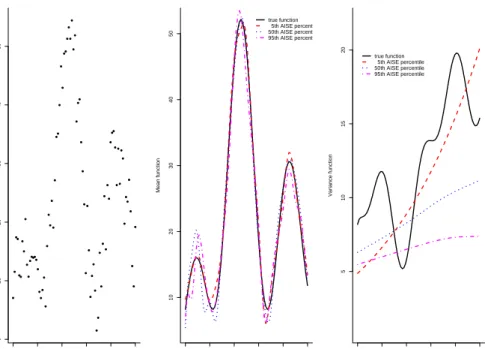
In this modelµ(x) = 8.2 + 45 sin(3x)(cos(7x))2 andγ(x) = 12 + 8 sin(−5x+ 0.1)(cos(8x+
0.1))2+ 2 log(4.2x+ 0.1). See Figure 4.1. We apply the estimation method using B-splines
of degrees pµ = pγ = 3, with a set of equally-spaced knots of dimensions kµ = 40 and kγ = 34. From 1000 simulated samples, we sort the 1000 AISE-values, and present in
Figure 4.1 the estimated mean and dispersion (variance) function corresponding to the 5th, the 50th and the 95th quantile of the AISE-values. From Figure 4.1 it can be seen that the estimates catch quite well the shape of the true curves. The estimation of the variance function is more difficult than that of the mean function, as expected.
0.0 0.2 0.4 0.6 0.8 1.0 0 10 20 30 40 50 60 (a) x y 0.0 0.2 0.4 0.6 0.8 1.0 10 20 30 40 50 (b) x Mean function true function 5th AISE percentile 50th AISE percentile 95th AISE percentile 0.0 0.2 0.4 0.6 0.8 1.0 5 10 15 20 (c) x Variance function true function 5th AISE percentile 50th AISE percentile 95th AISE percentile
Figure 4.1: Normal model with n = 250. (a) a simulated dataset; (b) the true mean function and (c) the true variance function, with representative estimates.
0.0 0.2 0.4 0.6 0.8 1.0 0 10 20 30 40 50 (a) x y 0.0 0.2 0.4 0.6 0.8 1.0 10 20 30 40 50 (b) x Mean function true function 5th AISE percentile 50th AISE percentile 95th AISE percentile 0.0 0.2 0.4 0.6 0.8 1.0 5 10 15 20 (c) x Variance function true function 5th AISE percentile 50th AISE percentile 95th AISE percentile
Figure 4.2: Normal model withn = 80. (a) a simulated dataset; (b) the true mean function and (c) the true variance function, with representative estimates.
Figure 4.2 depicts similar results as Figure 4.1, but now based on samples of size
0.0 0.2 0.4 0.6 0.8 0.0 0.5 1.0 1.5 2.0 2.5 3.0 3.5 (a)
Smoothing parameter for the mean
λµ Density 0 1000 2000 3000 4000 5000 0e+00 2e−04 4e−04 6e−04 8e−04 (b)
Smoothing parameter for the dispersion
λγ
Density
Figure 4.3: Normal model with n= 250. Estimated density for the GCV-selected λµ and λγ parameters.
this smaller sample size, the estimation of the mean function is still very accurate. The estimation of the variance function however is far less precise. Although, in general, the estimate catches the trend in the function, it often misses the bumps.
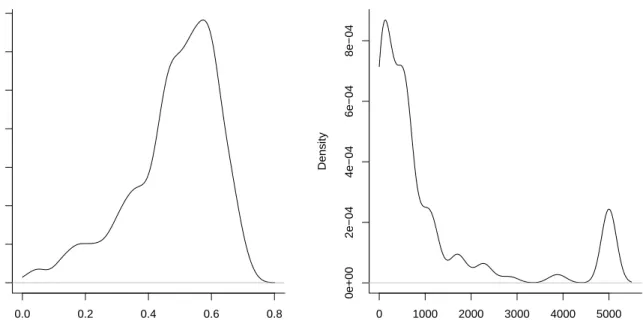
In Figure 4.3 we present the density of the selected smoothing values λµ and λγ,
obtained via the GCV-criteria as described in Section 3.2, for the 1000 samples of size
n = 250. Note that the selected λγ-values are far larger in magnitude and more spread
out than the selected λµ-values.
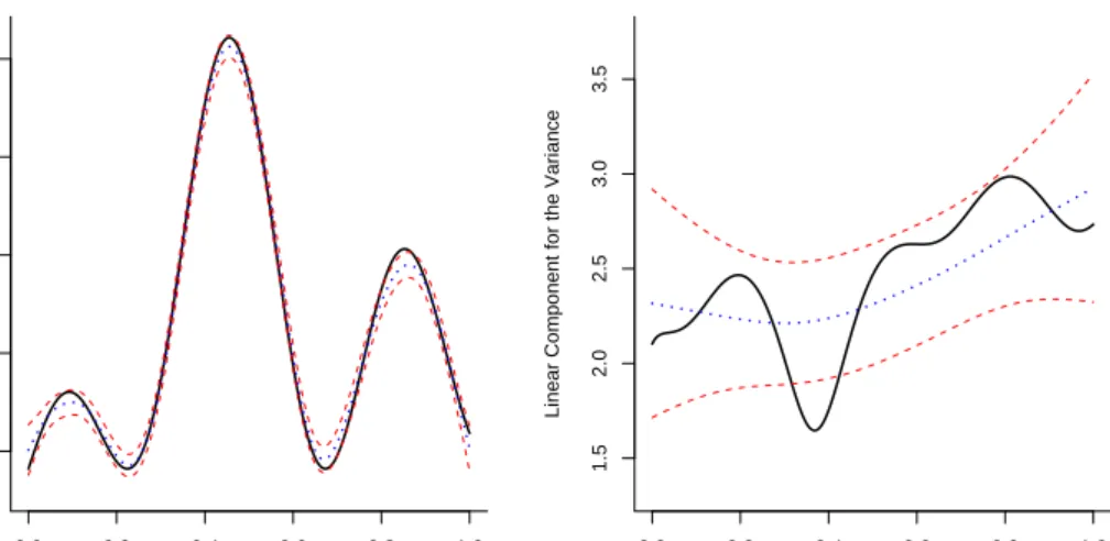
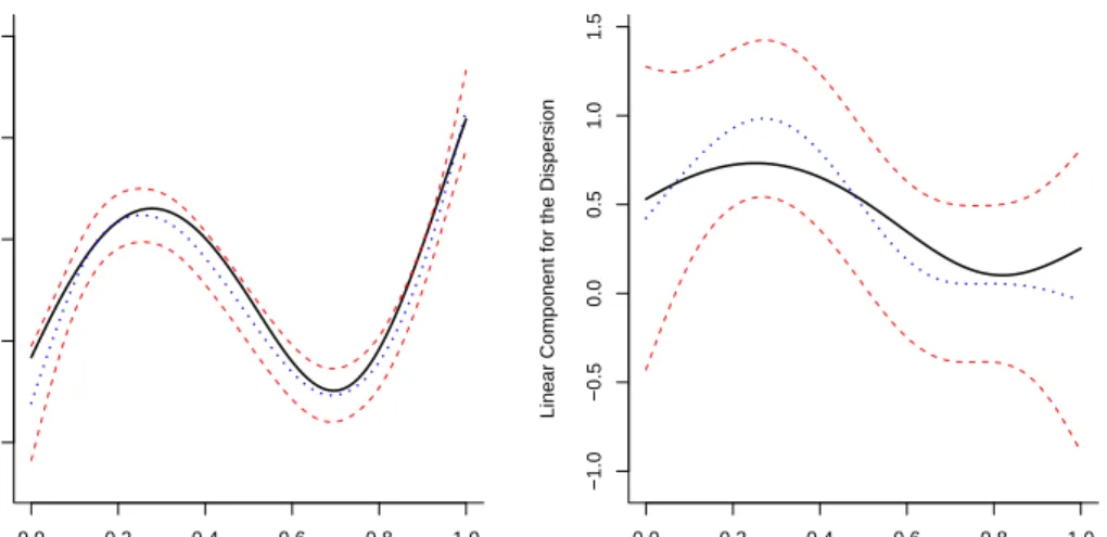
Of interest is also to look for constructing approximate confidence intervals. A pos-sibility is to rely on the Fisher information matrices derived in Section 3, and a large sample approximation by a normal distribution with mean the estimated target function and variance the generalization of the variance of a generalized linear model (as in formula (7) of Marx and Eilers (1998)). Confidence intervals for the components η(·) andξ(·) are presented in Figure 4.4 as short-dashed curves. Plotted are also the true functions (as solid curves) as well as the estimated curve corresponding to a median AISE performance (dotted curve). From Figure 4.4 (b) it is again seen that estimation of the dispersion function is a far more difficult problem than estimation of the mean function.
0.0 0.2 0.4 0.6 0.8 1.0 10 20 30 40 50 (a) x
Linear Component for the Mean
0.0 0.2 0.4 0.6 0.8 1.0 1.5 2.0 2.5 3.0 3.5 (b) x
Linear Component for the Variance
Figure 4.4: Normal model with n = 250: the estimate of the linear components η(·) and
ξ(·) corresponding to the median AISE values (dotted curve) for the mean (a) and the variance (b) function with 95% confidence intervals (short-dashed curves).
4.2
Poisson data
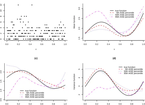
We now simulate from two different double Poisson models. For both models we take the same dispersion function γ(x) = 1.7−0.3x2 + 0.4 sin(6x) but we consider two different
mean functions. The mean function for the setting of Figure 4.5 equalsµ(x) = 26 + 40x+ 48(x−0.6)2 + 16 sin(6x) and is 25 times the mean function in the setting of Figure 4.6.
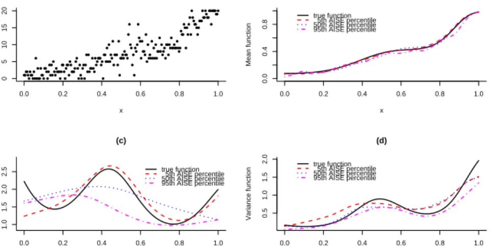
The true mean, dispersion and variance functions for both settings are depicted as solid curves in panels (b)—(d) of Figures 4.5 and 4.6. Typical simulated datasets are in panels (a) of Figures 4.5 and 4.6. We perform 1000 simulations of sample size n= 210. For the estimation procedure we use B-spline basis functions of degree pµ =pγ = 3 and
equally-spaced knots with kµ = 45 and kγ = 30. For both models, the method gives satisfactory
results: the general shape of the functions is well described by their estimates.
In Figure 4.7 approximate confidence intervals for the Poisson model with high mean function are presented. Note again the difference in width between the confidence intervals for the function η(·) on the one hand and the function ξ(·) on the other hand.
4.3
Binomial data
We now consider two binomial models. In presenting (and in analyzing) the data we use the proportion, rather than the actual number of successes over a certain number of trials in each experiment. The mean function is µ(x) = exp(−2.5 + 7.5x2+ 3.3x2sin(6x)/(1 +
0.0 0.2 0.4 0.6 0.8 1.0 30 40 50 60 70 80 90 (a) x y 0.0 0.2 0.4 0.6 0.8 1.0 40 50 60 70 (b) x Mean function true function 5th AISE percentile 50th AISE percentile 95th AISE percentile 0.0 0.2 0.4 0.6 0.8 1.0 1.0 1.5 2.0 2.5 3.0 (c) x
Dispersion function true function 5th AISE percentile 50th AISE percentile 95th AISE percentile 0.0 0.2 0.4 0.6 0.8 1.0 50 100 150 (d) x Variance function true function 5th AISE percentile 50th AISE percentile 95th AISE percentile
Figure 4.5: Poisson model with n = 210. (a) a simulated dataset, (b) the true (high) mean function, (c) the true dispersion function and (d) the true variance function, with representative estimates. 0.0 0.2 0.4 0.6 0.8 1.0 0 2 4 6 8 10 12 (a) x y 0.0 0.2 0.4 0.6 0.8 1.0 1.5 2.0 2.5 3.0 (b) x Mean function true function 5th AISE percentile 50th AISE percentile 95th AISE percentile 0.0 0.2 0.4 0.6 0.8 1.0 0.5 1.0 1.5 2.0 (c) x
Dispersion function true function
5th AISE percentile 50th AISE percentile 95th AISE percentile 0.0 0.2 0.4 0.6 0.8 1.0 2 3 4 5 (d) x Variance function true function 5th AISE percentile 50th AISE percentile 95th AISE percentile
Figure 4.6: Poisson model with n = 210. (a) a simulated dataset, (b) the true (low) mean function, (c) the true dispersion function and (d) the true variance function, with representative estimates.
0.0 0.2 0.4 0.6 0.8 1.0 3.6 3.8 4.0 4.2 4.4 (a) x
Linear Component for the Mean
0.0 0.2 0.4 0.6 0.8 1.0 −1.0 −0.5 0.0 0.5 1.0 1.5 (b) x
Linear Component for the Dispersion
Figure 4.7: High mean Poisson model with n= 210: the estimate of the components η(·)
and ξ(·) corresponding to the median AISE values (dotted curve) for the mean (a) and the dispersion (b) function with 95% confidence intervals (short-dashed curves).
exp(−2.5 + 7.5x2 + 3.3x2sin(6x)) and the dispersion function equals γ(x) = exp(0.8−
0.8 cos(4x+0.2) sin(6x)). The underlying mean, dispersion and variance function of a first model are depicted as solid curves in panels (b)—(d) in Figure 4.8. In this first model the constant number of trials is equal to 220. We draw 1000 samples of sizen = 200 from this model. A typical simulated dataset is depicted in Figure 4.8 (a). In the estimation procedure we take B-spline basis functions with pµ = pγ = 3 and kµ = 45 and kγ = 38
knots. The estimated curves corresponding to the 5th, the 50th and the 95th AISE-quantiles are presented in Figure 4.8. Again estimation of the mean is more precise than estimation of the dispersion function, but nevertheless the results are quite satisfactory. For a second binomial case we reduce the number of trials to 20. The results, obtained with the same B-spline bases functions and the same choices of knots, are still encouraging although less precise (see Figure 4.9).
Finally, confidence intervals for the functionη(·) andξ(·) are provided in Figure 4.10. The conclusions are similar as for the previous models.
4.4
Comparison with other methods
The approach of tackling estimation of mean and dispersion via the double exponential family and P-splines regression is quite appealing, since it allows for flexible modeling and can handle overdispersion as well as underdispersion. In this section we compare the
0.0 0.2 0.4 0.6 0.8 1.0 0 50 100 200 (a) x y 0.0 0.2 0.4 0.6 0.8 1.0 0.0 0.4 0.8 (b) x Mean function true function 5th AISE percentile 50th AISE percentile 95th AISE percentile 0.0 0.2 0.4 0.6 0.8 1.0 1.0 1.5 2.0 2.5 (c) x Dispersion function true function 5th AISE percentile 50th AISE percentile 95th AISE percentile 0.0 0.2 0.4 0.6 0.8 1.0 0.5 1.0 1.5 2.0 (d) x Variance function true function 5th AISE percentile 50th AISE percentile 95th AISE percentile
Figure 4.8: Binomial model with n = 200 and number of trials is 220. (a) a simulated dataset, (b) the true mean function, (c) the true dispersion function and (d) the true variance function, with representative estimates.
0.0 0.2 0.4 0.6 0.8 1.0 0 5 10 15 20 (a) x y 0.0 0.2 0.4 0.6 0.8 1.0 0.0 0.4 0.8 (b) x Mean function true function 5th AISE percentile 50th AISE percentile 95th AISE percentile 0.0 0.2 0.4 0.6 0.8 1.0 1.0 1.5 2.0 2.5 (c) x Dispersion function true function 5th AISE percentile 50th AISE percentile 95th AISE percentile 0.0 0.2 0.4 0.6 0.8 1.0 0.5 1.0 1.5 2.0 (d) x Variance function true function 5th AISE percentile 50th AISE percentile 95th AISE percentile
Figure 4.9: Binomial model with n = 200 and number of trials is 20. (a) a simulated dataset, (b) the true mean function, (c) the true dispersion function and (d) the true variance function, with representative estimates.
proposed estimation method with other methods for variance or dispersion estimation available in the literature.
A first question one might ask is what can be gained by allowing for a dispersion that changes with the covariate value x, as opposed to just modeling an additional dispersion parameter.
A second question is how the proposed method compares to other methods for esti-mating a dispersion function (or a variance function in the normal model). In this section
0.0 0.2 0.4 0.6 0.8 1.0 −6 −4 −2 0 2 4 6 8 (a) x
Linear Component for the Mean
0.0 0.2 0.4 0.6 0.8 1.0 −0.5 0.0 0.5 1.0 (b) x
Linear Component for the Dispersion
Figure 4.10: Binomial model with n = 200 and the number of trials is 220: the estimate of η(·) and ξ(·) corresponding to the median AISE values (dotted curve) for the mean (a) and the dispersion (b) function with 95% confidence intervals (short-dashed curves).
we compare our approach with the mixed model approach of Rigby and Stasinopoulos (2005). For the normal model, when estimating a variance function, we also compare with a difference type of variance estimation. See for example Hall et al. (1990).
In difference-based estimation of the variance function, one needs to choose a difference sequence {dj}, which is a sequence of real numbers such that Pdj = 0 and Pd2j = 1.
For a given strictly positive integer m, put dj = 0 for j > m, and calculate the sequence
of differences of subsequent Y-observations (v1,· · ·, vn−m) where vi = Pmj=0djyi+j for
i = 1,· · ·n −m. Variance estimators are then based on the sequence (v1,· · · , vn−m),
with the simplest example its empirical variance. In the comparison we use a P-spline to estimate the variance from the sequence (v1,· · · , vn−m). This difference-based variance
estimation depends on the choice of the difference order m. We present results for the method when fixing the order m = 3, but for comparison reasons also include results obtained when choosing the optimal m from the set of values 1,2,· · · ,6. More precisely, for each sample we calculate the difference-based estimator for all values ofm, and report on the estimator for which the AISE value if minimal. Note that when doing so, we use the information on the true function when selecting the optimalmfor the sample at hand. Rigby and Stasinopoulos’ (2005) GAMLSS framework also allows for estimation of the mean and the variance/dispersion function. Thegamlssfunction of thegamlssR package (Stasinopoulos and Rigby (2007)) though uses by default smoothing splines with a fixed
number of degrees of freedom. For comparison purpose we also use P-splines in the Rigby and Stasinopoulos (2005) method applying the pb function, taking the same number of knots, the same degree and the same order of difference operator in both methods.
When dealing with overdispersed data one possibility is to estimate the one-parameter exponential family dispersion parameterφ as a constant via the deviance residuals. If the interest instead is to estimate the dispersion as a function of the covariate, different meth-ods can be used. A common approach is to make some distributional assumptions on the location parameter so that the data are modeled via specific two-parameter distributions which allow the dispersion to be non constant. In particular overdispersed count data are modeled via a negative binomial distribution and overdispersed proportion data via a beta-binomial distribution. These modeling approaches are also used by Rigby and Stasinopoulos (2005). Although the double exponential family and the hierarchical mod-els both allow to model the dispersion, the actual assumed distribution can be quite different. For a full and fair comparison between the different methods, we therefore present results when simulations are done under the two different schemes (double expo-nential family and either a negative binomial or a beta-binomial) in such a way that the mean and variance function would be the same.
To summarize, we present results on AISE values for the following methods:
Const.Var or Const.Disp: results obtained from the proposed method but assuming
the variance or dispersion to be a constant;
def: proposed estimation procedure, starting from a double exponential family; rs: method of Rigby and Stasinopoulos (2005);
diffCh:difference-based estimation of the variance with optimal choice of the difference
order m in each simulated sample;
diff3: difference-based estimation of the variance withm = 3,
when either generating data from an double exponential family (DEF) model or from a negative binomial or a beta-binomial (for the Poisson or binomial case respectively).
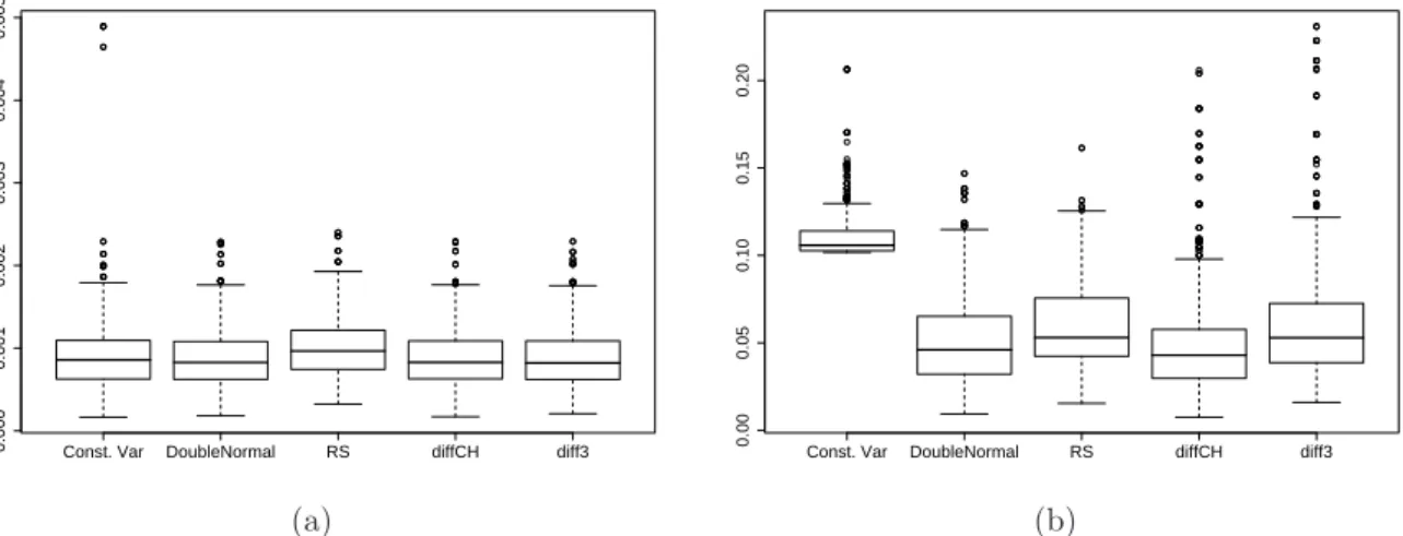
The boxplots reporting on the comparisons of the methods are given in Figures 4.11— 4.13. For the normal model, it can be seen from Figure 4.11 (a) that estimation of the mean function is only slightly affected by the method. More differences can be noticed for the variance estimation in Figure 4.11 (b): estimating the variance function as a constant gives very high AISE values. Not surprising is also that the difference-based variance estimation
(diffCH ) has lower AISE values. The other three estimationprocedures give com-parable results, with the double normal method performing somewhat better than the others.
Const. Var DoubleNormal RS diffCH diff3
0.000 0.001 0.002 0.003 0.004 0.005
AISE for the mean: Normal of size 250
(a)
Const. Var DoubleNormal RS diffCH diff3
0.00
0.05
0.10
0.15
0.20
AISE for the variance: Normal of size 250
(b)
Figure 4.11: Normal model with n = 250: boxplots of the AISE values for the mean (a) and the dispersion (b) for different variance estimation procedures.
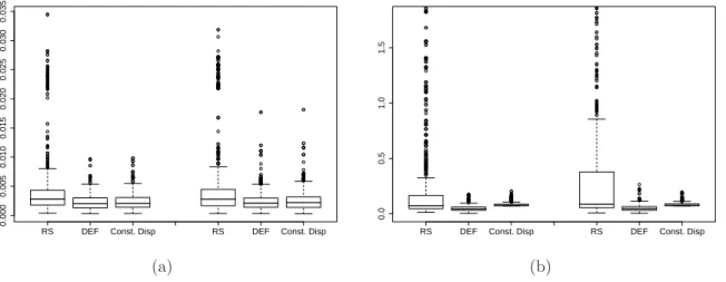
RS DEF Const. Disp RS DEF Const. Disp
0.00
0.05
0.10
0.15
AISE for the mean: Poisson with low mean
(a)
RS DEF Const. Disp RS DEF Const. Disp
0.0 0.1 0.2 0.3 0.4 0.5
AISE for the dispersion: Poisson with low mean (outliers not shown)
(b)
Figure 4.12: Low mean Poisson model with n = 210: boxplots of the AISE values for the mean (a) and the dispersion (b) for different dispersion estimation procedures. Data are generated either via a DEF (left group of boxplots) or a negative binomial (right group of boxplots).
In Figure 4.12 results are presented for the Poisson model with low mean. First of all we notice that the performance of the different methods is comparable whether the data are generated via a DEF or a negative binomial. Also, not surprisingly, estimating the dispersion as a constant always leads to higher AISE values for the dispersion, and in the
case of higher mean (results not reported here) estimating the dispersion as a function rather than as a constant, also leads to noticeably better performance in estimation of the mean function. Comparing the hierarchical approach of Rigby and Stasinopoulos (2005) with the proposed DEF approach we see that the performances are quite comparable with a slight dominance of the proposed approach.
RS DEF Const. Disp RS DEF Const. Disp
0.000 0.005 0.010 0.015 0.020 0.025 0.030 0.035
AISE for the mean: Binomial with low number of trials
(a)
RS DEF Const. Disp RS DEF Const. Disp
0.0
0.5
1.0
1.5
AISE for the dispersion: Binomial with low number of trials (outliers not shown)
(b)
Figure 4.13: Binomial model with n = 200 and number of trials is 20: boxplots of the AISE values for the mean (a) and the dispersion (b) for different dispersion estimation procedures. Data are generated either via a DEF (left group of boxplots) or a beta-binomial (right group of boxplots).
As far as proportion data are concerned we can see in Figure 4.13 the effect of the different dispersion estimation methods on data generated either via a DEF or a beta-binomial with low number of trials. Here the DEF approach performs much better than the beta-binomial approach for both simulation schemes. It should be mentioned that in order to have a variance for the data corresponding to the true known function, the true values for the scale parameter of a beta-binomial are very close to the limiting value and vary very little. This for sure makes the estimation more complex and could partially explain the poor performance. At the same time it also sheds some light on how different the two approaches are. In particular values ofγ close to 1 correspond to the limiting value of the scale parameter of the beta-binomial distribution and in general the beta-binomial approach would behave badly in cases in which part of the data would be underdispersed. In contrast, the proposed approach can deal with underdispersion, overdispersion and even a combination of these.
5
Data examples
We now illustrate the proposed estimation procedure on several datasets. Again we present results for continuous data, counts and proportions.
15 20 25 30 35 40 45 50 0 2 4 6 8 10 12 (a) Age
# of induced abortion per 1000 women
15 20 25 30 35 40 45 50 0.00 0.05 0.10 0.15 (b) Age Deviance
Figure 5.1: The Italian induced abortions data: (a) mean and (b) dispersion function estimation (kµ = 6 kγ = 5, pµ = 3 pγ = 3).
5.1
The Italian Induced Abortions data
15 20 25 30 35 40 45 50 −2 −1 0 1 2 (a) Age Deviance residuals 15 20 25 30 35 40 45 50 −2 −1 0 1 2 (b) Age
Standardized deviance residuals
Figure 5.2: The Italian induced abortions data: (a) unstandardized and (b) standardized deviance residuals.
The National Institute of Statistics in Italy (ISTAT) collects different information on induced abortion in order to monitor the phenomenon. Among the collected information
15 20 25 30 35 40 45 50 −4 −2 0 2 (a) Age
log(# of induced abortion per 1000 women)
15 20 25 30 35 40 45 50 −14 −12 −10 −8 −6 −4 −2 (b) Age log(Deviance)
Figure 5.3: The Italian induced abortions data. The estimated functions (a) η(·) and (b)
ξ(·) (solid curves) with approximate confidence intervals (dashed curves).
is the total number of induced abortions on women of a specific age for each Italian region in the year 2006. We present here data for the Veneto region standardized in such a way that we have the counts of induced abortions per 1000 women as a dependent variable. The data, with an estimate for the mean, and the calculated deviance residuals, with an estimate of the dispersion function, are shown in Figure 5.1. When using a Poisson model we expect the variance of the data to be the same as the mean, but here we notice that the variance of the data is always considerably smaller than the mean (underdispersion). From the dispersion function estimate in Figure 5.1 (b) it is seen that there is a quite strong underdispersion over the whole covariate range. In Figure 5.2 we present the unstandardized (considering the dispersion as constant) and the standardized residuals (standardized using the estimated dispersion). Figure 5.2 (b) gives a clear indication that the estimation of the dispersion function performed quite well.
In Figure 5.3 (a) the estimated function ˆη(·) and its corresponding approximate confi-dence intervals are given. Figure 5.3 (b) depicts the estimation forξ(·) with approximate confidence intervals.
5.2
The Fabric data
A classical dataset for overdispersed Poisson data is the fabric dataset, containing 32 observations of the number of faults in rolls of fabric, and the logarithm of the length of each roll. See Hinde (1982). The data, with an estimate for the mean, and the calculated deviance residuals, with an estimate of the dispersion function, are shown in Figure 5.4.
The deviance residuals seem indeed to be dependent on the length of the roll. In Figure 5.5, we plot the unstandardized and standardized residuals. Figure 5.5 (b) shows no or less dependence on the covariate. Note that in this data example, the estimated dispersion function ˆγ(x) goes from values less than one to values bigger than one, i.e. is crossing over from underdispersion to overdispersion.
5.0 5.5 6.0 6.5 0 5 10 15 20 25 (a) log(roll length) Number of faults 5.0 5.5 6.0 6.5 0 2 4 6 8 (b) log(roll length) Deviance
Figure 5.4: The Fabric data: (a) mean and (b) dispersion function estimation (kµ = 7
kγ = 5, pµ= 3 pγ = 2). 5.0 5.5 6.0 6.5 −2 −1 0 1 2 (a) log(roll length) Deviance residuals 5.0 5.5 6.0 6.5 −2 −1 0 1 2 (b) log(roll length)
Standardized deviance residuals
Figure 5.5: The Fabric data: (a) unstandardized and (b) standardized deviance residuals.
5.3
The Hospital stay data
The Hospital stay data concern a study at the Hospital del Mar in Barcelona during the years 1988 and 1990. See Alonso et al. (1996). The data set contains, among
other measurements, the number of inappropriate days spent out of the whole stay in the hospital in the year 1988 (750 patients) and 1990 (633 patients). For this illustration we focus our attention on the data concerning year 1988, and we are interested in studying the relationship between the age of the patient and the proportion of inappropriate days out of all days spent in the hospital. We model the data as a double binomial family. The estimated mean and dispersion function are shown in Figure 5.6. Figure 5.7 (a) indicates that the variance of the data increases with the age of the patients, while the standardized residuals Figure 5.7 (b) no longer shows this dependence.
20 40 60 80 100 0.0 0.2 0.4 0.6 0.8 1.0 (a) Age
Proportion of inappopriate days in hospital
20 40 60 80 100 0 50 100 150 (b) Age Deviance
Figure 5.6: The Hospital stay data: (a) mean and (b) dispersion function estimation (kµ = 52 kγ = 44, pµ= 3 pγ = 2). 20 40 60 80 100 −5 0 5 10 (a) Age Deviance residuals 20 40 60 80 100 −5 0 5 10 (b) Age
Standardized deviance residuals
Figure 5.7: The Hospital stay data: (a) unstandardized and (b) standardized deviance residuals.
5.4
The low iron rat data
A known dataset concerning overdispersed binomial data is the low iron rat data described by Moore and Tsiatis (1991). An experiment is conducted to see whether the level of hemoglobin in the blood has an effect on the number of dead fetus found in the litter. 58 rats are given an iron supplement, at different dose levels; after 3 weeks they are sacrificed and the proportion of dead fetus on the total size of the litter is recorded. The data, with an estimate for the mean and the dispersion functions are shown in Figure 5.8. The decreasing shape of the deviance seems to be well captured by the estimated function. The plots of the unstandardized and the standardized residuals, in Figure 5.9, convince us of the necessity of modeling the dispersion function as a function of the covariate.
4 6 8 10 12 14 16 0.0 0.2 0.4 0.6 0.8 1.0 (a) Hemoglobin
Proportion of dead foetus
4 6 8 10 12 14 16 0 5 10 15 20 (b) Hemoglobin Deviance
Figure 5.8: The low iron rat data: (a) mean and (b) dispersion function estimation (kµ =
kγ = 11, pµ=pγ = 2).
These data have been also analyzed by Aerts and Claeskens (1997) via a local beta-binomial model and by Nott (2006), who used a DEF approach with Bayesian semipara-metric fitting. The estimated mean and dispersion functions seen in Figure 5.8 are very similar to the ones found by the other authors.
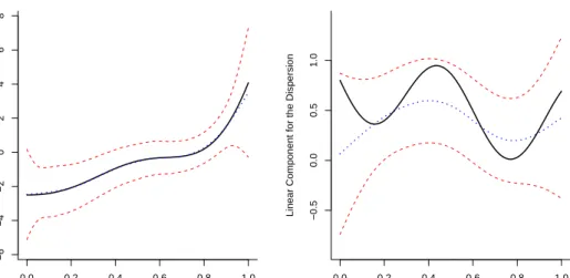
The estimated curvesη(·) andξ(·) together with their approximate confidence intervals are depicted in respectively Figure 5.10 (a) and Figure 5.10 (b). Note that the pointwise confidence intervals for η(·) are wider at the left end of the support (since there the variability in the data is larger).
4 6 8 10 12 14 16 −6 −4 −2 0 2 4 6 (a) Hemoglobin Deviance residuals 4 6 8 10 12 14 16 −6 −4 −2 0 2 4 6 (b) Hemoglobin
Standardized deviance residuals
Figure 5.9: The low iron rat data: (a) unstandardized and (b) standardized deviance residuals. 4 6 8 10 12 14 16 −10 −5 0 5 10 (a) Hemoglobin
logistic(Proportion of dead foetus)
4 6 8 10 12 14 16 −4 −2 0 2 (b) Hemoglobin log(Deviance)
Figure 5.10: The low iron rat data. The estimated functions (a) η(·) and (b) ξ(·) (solid curves) with approximate confidence intervals (dashed curves).
5.5
The Lidar data
An example of normal data is the Lidar dataset, which is discussed in Ruppert et al.
(2003), among others. Lidar (Light detection and ranging) is a technique to detect chem-ical compounds in the atmosphere. The dataset contains the data coming from a Lidar experiment: 221 observations of the distance the light traveled before being reflected back to its source, and of the logarithm of the ratio of received light from two laser sources. In Figure 5.11 we plot the data and the obtained estimates for the mean and the variance function. The data show indeed a non-constant variance and the estimate seems to catch the increasing shape of the function. Figure 5.12 gives a clear indication that the
esti-mation of the variance function performed quite well. Ruppert et al. (2003) also find an increasing shape for the variance function of these data.
400 450 500 550 600 650 700 −0.8 −0.6 −0.4 −0.2 0.0 (a) Range Logratio 400 450 500 550 600 650 700 0.00 0.02 0.04 0.06 0.08 (b) Range Squared residuals
Figure 5.11: The Lidar data: (a) mean and (b) variance function estimation (kµ = 45
kγ = 35, pµ=pγ = 3). 400 450 500 550 600 650 700 −2 −1 0 1 2 (a) Range Residuals 400 450 500 550 600 650 700 −2 −1 0 1 2 (b) Range Standardized residuals
Figure 5.12: The Lidar data: (a) unstandardized and (b) standardized residuals.
Figures 5.13 (a) and (b) show the estimated functions η(·) and ξ(·) respectively, to-gether with their approximate confidence intervals.
6
Further discussion
As was noted in Lee and Nelder (2000), the double exponential family leads to identical inference as the extended quasi likelihood approach (see McCullagh and Nelder (1989)).
400 450 500 550 600 650 700 −0.8 −0.6 −0.4 −0.2 0.0 (a) Range Logratio 400 450 500 550 600 650 700 −15 −10 −5 (b) Range log(Squared residuals)
Figure 5.13: The Lidar data. The estimated functions (a) η(·) and (b) ξ(·) (solid curves) with approximate confidence intervals (dashed curves).
In a similar manner one can consider an extended quasi likelihood approach in the current context. This has been done by the authors but for brevity we do not elaborate on this in the paper.
One might wonder whether it is possible to select the two smoothing parameters λµ
andλγ simultaneously. A first task then is to define an appropriate type of bivariate GCV
criterion. Following the idea behind the univariate GCV criteria developed in Section 3 one needs to define the deviance of the model: start from the likelihood in (3.1) and take
θS =g−1(y) and γS =d(y, θ) to be the choice of θ and γ corresponding to the saturated
model. As the total number of degrees of freedom we take the sum of the equivalent number of degrees of freedom needed when fitting the mean and the dispersion function. This leads to GCV(λµ, λγ) = n X i=1 log ˆγλ γ(xi)−logd(yi, ˆ θλµ(xi)) +d(yi, ˆ θλµ(xi))/γλˆ γ(xi) (n−df(λγ)−df(λµ))2 . (6.1)
Minimizing GCV(λµ, λγ) with respect to λµ and λγ simultaneously will then give
direct choices for both smoothing parameters. The optimization can be done numerically using theoptimfunction of R. Experiences show that optimization of GCV(λµ, λγ) is not
straightforward: the function often presents local minima in different directions, so that the minimization process becomes difficult and strongly dependent on the provided initial values. Alternatively, one can do a two-dimensional grid search, but this at the cost of a considerable increase in computing time. A grid search also faces the same problem of
several local minima.
As an illustration we present in Figure 6.1 boxplots of the AISE values for the mean and the dispersion estimation in the normal model when choosing the smoothing parameters either in separate steps (left-hand side boxplots) or via the bivariate criterion (right-hand side boxplots). As can be seen there is no gain from considering the bivariate GCV criterion. Similar results (not presented here) were obtained for the other simulation models. Since the bivariate GCV criterion also seems to suffer from the above mentioned drawbacks, we do not recommend its use.
GCV(λµ) GCV(λµ,λγ) 0.000 0.001 0.002 0.003 0.004 0.005
AISE for the mean: Normal of size 250 (outliers not shown)
(a) GCV(λγ) GCV(λµ,λγ) 0.00 0.05 0.10 0.15 0.20 0.25
AISE for the variance: Normal of size 250 (outliers not shown)
(b)
Figure 6.1: Normal model with n = 250: boxplots of the AISE-values for the mean (a) and the variance (b) estimation when choosing the smoothing parameters in two different steps (left boxplots) or simultaneously (right boxplots).
Other selection criteria for choosing λµ and λγ have been explored, among which
Akaike’s Information (AIC) criteria (univariate and bivariate). None of these however outperformed the univariate GCV criteria of Section 3. Nevertheless, these criteria are not without problems since the optimization problems can be hard, in particular with respect to the smoothing parameter selection for the dispersion estimation. More research is needed for developing better selection rules.
In this paper the mean and dispersion function are estimated nonparametrically using P-spline techniques. Other smoothing techniques such as local polynomial fitting could also serve as a basis here. So far no theoretical studies have been done for establishing the rate of convergence of the dispersion function estimator. Concerning estimation of the mean regression function using penalized splines techniques, there is recent work dealing with asymptotic theory. This includes work by Li and Ruppert (2008) who establish the asymptotic distribution of penalized mean regression estimators. Further, Kauermann
approach and Laplace approximations for their asymptotic study. Claeskens et al. (2009) study asymptotic properties of a class of penalized spline regression estimators. Asymp-totic results focusing on the choice of the difference type of penalty are provided in Gijbels and Verhasselt (2010a,b). Some studies on rates of convergence for variance function es-timation (in general) can be found in the literature, including the works by Hall and Carroll (1989), Ruppert et al. (1997), Fan and Yao (1998) and Wang et al. (2008). These papers in particular study the effect of mean estimation on variance estimation, and reveal, for example, that the rate of convergence of the variance estimator is similar to that of the mean estimator provided the mean function has some minimal degree of smoothness. It would be interesting to investigate the effect of the mean estimation on the dispersion function estimation, and to establish asymptotic theory for the dispersion function estimate.
In Section 4 we provide approximate confidence intervals. Of interest would also be to develop a method for constructing confidence bands. This is an open research issue.
Acknowledgements
The authors thank the reviewers for their valuable comments which led to additional interesting investigations and an improved presentation. Support from the GOA/07/04-project of the Research Fund KULeuven is gratefully acknowledged, as well as support from the IAP research network nr. P6/03 of the Federal Science Policy, Belgium. The authors thank Dr Danie Uys for helpful discussions.
References
Aerts, M. and Claeskens, G. (1997). Local polynomial estimation in multiparameter likelihood models. Journal of the American Statistical Association, 92, 1536–1545. Alonso, J., Mu˜noz, A. and Ant´o, J. M. (1996). Using length of stay and inactive days in the hospital to assess appropriateness of utilization in Barcelona, Spain. Journal of Epidemiology and Community Health, 50, 196–201.
de Boor, C. (2001). A Practical Guide to Splines. Revised Edition. Springer, Berlin. Carroll, R.J. and Ruppert, D. (1988). Transformation and Weighting in Regression,
Chapman and Hall: New York.
Claeskens, G., Krivobokova, T. and Opsomer, J.D. (2009). Asymptotic properties of penalized spline estimators. Biometrika, 96, 529–544.
Davidian, M. and Carroll, R.J. (1987). Variance function Estimation. Journal of the American Statistical Association, 82, 1079–1091.
Davidian, M. and Carroll, R.J. (1988). A note on Extended Quasi-likelihood. Journal of the Royal Statistical Society, Series B, 50, 74–82.
Dey, D.K., Galfand, A.E. and Peng, F. (1997). Overdispersed generalized linear models.
Journal of Statistical Planning and Inference,64, 93–107.
Eilers, P.H.C. and Marx, B.D. (1996). Flexible Smoothing with B-splines and Penalties.
Statistical Science,11, 89–121.
Efron, B. (1986). Double Exponential Families and their Use in Generalized Linear Regression. Journal of the American Statistical Association, 81, 809–721.
Fan, J. and Yao, Q. (1998). Efficient estimation of conditional variance functions in stochastic regression. Biometrika, 85, 645–660.
Galfand, A.E. and Dalal, S.R. (1990). A note on Overdispersed Exponential Families.
Biometrika,77, 55–64.
Gijbels, I. and Verhasselt, A. (2010a). P-splines regression smoothing and difference type of penalty. Statistics and Computing, to appear.
DOI:10.1007/s11222-009-9140-0
Gijbels, I. and Verhasselt, A. (2010b). Regularisation and P-splines in generalised linear models. Journal of Nonparametric Statistics, to appear.
DOI: 10.1080/10485250903365900
Hall, P. and Carroll, R.J. (1989). Variance function estimation in regression: the effect of estimating the mean. Journal of the Royal Statistical Society, Series B,51, 3–14.
Hall, P., Kay, J. and Titterington, D. (1990). Asymptotically optimal difference-based estimation of variance in nonparametric regression. Biometrika, 77, 521–528.
Hinde, J. (1982). Compound Poisson regression mode: inGLIM82; InProceedings of the International Conference on Generalized Linear Models, ed. Gilchrist, R., 109–121, Springer: New York.
Hinde, J. and Dem´etrio C.G.B. (1998). Overdispersion: Models and estimation. Com-putational Statistics & Data Analysis, 27, 151–170.
Kauermann, G. , Krivobokava, T. and Fahrmeir, L. (2009). Some asymptotic results on generalized penalized spline smoothing. Journal of the Royal Statistical Society, Series B, 71, 487–503.
Lee, Y. and Nelder, J. A. (1996). Hierarchical generalized linear models (with discussion).
Journal of the Royal Statistical Society, Series B,58, 619–678.
Lee, Y. and Nelder, J. A. (2000). The relationship between double-exponential fami-lies and extended quasi-likelihood famifami-lies, with application to modelling Geissler’s human sex ratio data. Applied Statistics, 49, 413–419.
Lee, Y. and Nelder, J. A. (2001). Hierarchical generalized linear models: a synthe-sis of generalized linear models, random-effect models and structured dispersions.
Biometrika,88, 987–1006.
Li, Y. and Ruppert, D. (2008). On the asymptotics of penalized splines. Biometrika,
95, 415–436.
Marx, B.D and Eilers, P.H.C. (1998). Direct generalized additive modeling with penal-ized likelihood. Computational Statistics & Data Analysis,28, 193–209.
McCullagh, P. and Nelder, J.A. (1989). Generalized Linear Model, Chapman and Hall: London.
Moore, D. F. and Tsiatis, A. (1991). Robust estimation of the variance in Moment Methods for Extra-Binomial and Extra-Poisson Variation. Biometrics, 47, 383– 401.
Nelder, J.A. and Lee, Y. (1992). Likelihood, Quasi-likelihood and Pseudolikelihood: Some Comparisons. Journal of the Royal Statistical Society, Series B,54, 273–284.
Nelder, J.A. and Pregibon, D. (1987). An extended quasi-likelihood function. Biometrika,
74, 221–232.
Nott, D. (2006). Semiparametric estimation of mean and variance functions for non-Gaussian data. Computational Statistics, 21 603–620.
Rigby, R. A. and Stasinopoulos, D. M. (2005). Generalized additive models for location, scale and shape. Applied Statistics, 54, 507–554.
Ruppert, D., Wand, M. and Carroll, R. J. (2003). Semiparametric Regression. Cam-bridge University Press.
Ruppert, D., Wand, M.P. Holst, U. and H¨ossjer, O. (1997). Local polynomial variance-function estimation. Technometrics, 39, 262–273.
Stasinopoulos, D. M. and Rigby, R.A. (2007). Generalized additive models for location scale and shape (GAMLSS) in R. Journal of Statistical Software, 23, Issue 7. Wahba, G. (1990). Spline Models for Observational Data. Philadelphia: SIAM.
Wang, L., Brown, L.D., Cai, T.T. and Levine, M. (2008). Effect of mean on variance function estimation in nonparametric regression The Annals of Statistics, 36, 646– 664.