Confidence intervals for
high-dimensional partially
linear single-index models
Gueuning T, Claeskens G.
KBI_1611
Confidence intervals for high-dimensional partially linear
single-index models
Thomas Gueuning and Gerda Claeskens
ORSTAT and Leuven Statistics Research Center KU Leuven, Faculty of Economics and Business
Naamsestraat 69, 3000 Leuven, Belgium
[email protected], [email protected] Abstract
We study partially linear single-index models where both model parts may contain high-dimensional variables. While the single-index part is of fixed dimension, the dimension of the linear part is allowed to grow with the sample size. Due to the addition of penalty terms to the loss function in order to provide sparse estimators, such as obtained by lasso or SCAD, the construction of confidence intervals for the model parameters is not as straightforward as in the classical low-dimensional data framework. By adding a correction term to the penalized estimator a desparsified estimator is obtained for which asymptotic normality is proven. We study the construction of confidence intervals and hypothesis tests for such models. The simulation results show that the method performs well for high-dimensional single-index models.
Keywords: high-dimensional data; single-index model; regularized estimation; sparsity; asymptotic normality; confidence interval
1
Introduction
A partially linear single-index model is a semi-parametric model which can be written as Y =
η(Z⊤α)+X⊤β+ϵ, whereηis a one-dimensional unknown function andZ,Xare covariate vectors of dimension p and q, respectively, such that the mean zero random error ϵ is independent of (Z, X). The underlying idea is that when the linearity assumption may not be valid for all covariates the introduction of an unknown function allows to overcome this problem. We focus on the high-dimensional case where the number of covariatesp+q may exceed the sample size
n. In this paper, we consider pas fixed and allow q to grow with n.
We show how to construct a desparsified version of a penalized estimator of the high-dimensional parameters (α, β) of the partially linear single-index model, and we establish the asymptotic dis-tribution of this desparsified estimator. The main purpose of desparsifying a penalized estimator that is obtained under the assumption of sparsity is that the construction of confidence inter-vals becomes thus possible for all of the components of the parameter vector, also for the ones asymptotically consistently estimated by zero due to the penalized estimation and which result
in a point mass at zero in the asymptotic distribution. Van de Geer et al. (2014) introduce such desparsified lasso estimators in the context of linear and generalized linear models and obtain their asymptotically normal distribution. This is done by writing the Karush-Kuhn-Tucker con-ditions which define the lasso estimator. It is then possible to find a de-biased lasso estimator and to characterize its asymptotic distribution under suitable conditions including a stricter sparsity condition. The construction of confidence intervals for the model parameters is then straightfor-ward. Note that for linear models, their method is the same one as that from Zhang and Zhang (2014). Javanmard and Montanari (2014) also provide a desparsified estimator in the context of the linear model. The main difference with the approach of van de Geer et al. (2014) is that they do not make any assumption on the sparsity level of the precision matrix.
Waldorp (2015) used the desparsified lasso for comparing high-dimensional graphical models. He obtained desparsified estimators for the coefficients of the precision matrices of the graphical models and constructed hypothesis tests based on the asymptotic distribution of these estima-tors. Lu et al. (2015) also used the desparsifying idea for constructing confidence bands for a class of nonparametric sparse additive models.
The use of a single index as opposed to a full p-variate nonparametric function estimation ef-fectively circumvents the curse of dimensionality. In a low dimensional setting, the (partially linear) single-index model has been studied by Carroll et al. (1997), Horowitz (1998), Xia et al. (1999), Yu and Ruppert (2002) and Xia and H¨ardle (2006), among others. The fitting process involves estimation of the parameters and of the unknown functionη. Different fitting methods have been introduced, most of them use kernel smoothing. Liang et al. (2010) and Wang et al. (2010) used the local linear regression technique introduced by Fan and Gijbels (1996) to esti-mate η. The resulting estimators have good theoretical properties regarding consistency and convergence rates. To deal with high dimensional covariate vectors, Liang et al. (2010) used a smoothly clipped absolute deviation penalty (SCAD, see Fan and Li (2001)). They obtain a profile least-squares function to minimize, similarly to the linear model case. Ma and Zhu (2013) study such models under heteroscedasticity.
Our goal is to provide confidence intervals for the high-dimensional parameter vector in the partially linear single index model and to determine which conditions (design, sparsity, etc.) are necessary to make this construction possible, the challenging part being to be able to tackle the presence of the unknown function η. In a fixed dimension framework, Zhu and Xue (2006) introduced the empirical likelihood to construct confidence regions. Further, Zhang et al. (2012) developed a dimension reduction approach for estimation in a partially linear single-index model (PLSIM) with diverging number of parameters in both the linear and the single-index part but needed the strong condition max(p, q) =o(n1/3) excluding the p+q > n case. Our method for
constructing confidence intervals and regions works in the high-dimensional frameworkp+q > n
withp fixed (potentially larger than n) andq growing withn.
First, in Section 2, we describe a method for estimating a partially linear single-index model. Our main results are in Section 3 where we construct a desparsified estimator and study its asymptotic distribution. Section 4 describes the construction of confidence intervals and regions together with ways to perform hypothesis testing following from the theoretical study. Section 5 deals with computational choices. Further, Section 6 reports on simulation studies to assess the finite sample performance of the desparsified estimator. In Section 7 we illustrate our method on a dataset to study the Bardet-Biedl disease in a rat population. This disease is linked to genetic mutations and also affects humans, provoking several dysfunctions. The dataset comprises of 120 observations and 200 variables. Section 8 concludes. All proofs are contained in Section 9.
2
Estimation for partially linear single-index model
Let {(Yi, Zi, Xi), i= 1, . . . , n} be a sample generated by the partially linear single-index model Y =η(Z⊤α0) +X⊤β0+ϵ,
where η : R → R is an unknown differentiable function, ϵ ∼ N(0, σϵ2), α0 ∈ Rp and β0 ∈ Rq
are the regression parameters and Z and X are, respectively, p-dimensional and q-dimensional covariate vectors. The error term ϵand the covariatesZ, X are independent. For identifiability reason, we assume that∥α0∥= 1 and that the first non-zero entry ofα0 is positive. We consider
p as fixed and allow q to grow with n. The casep+q > ncorresponds to the high-dimensional data framework. We denote by ξ= (α⊤, β⊤)⊤ thep+q−dimensional vector of parameters. Several estimation approaches have been introduced in the literature. In this paper, we use the profile least-squares procedure presented in Liang et al. (2010). For the paper to be self-contained, we here summarize the main ingredients. This approach uses the local linear regres-sion technique to estimate η, that is, an estimator of η(u) is obtained by the minimization of
n
∑
i=1
{a+b(Zi⊤α−u) +Xi⊤β−Yi}2Kh(Zi⊤α−u), (1)
with respect to a and b, where Kh(·) =h−1K(·/h), K(·) is a kernel function and h is a
band-width. The minimizer (ˆa,ˆb) of (1) is an estimator of (η(u), dη(u)/du). It can be shown (see Fan and Gijbels (1996)) that
ˆ η(u, ξ) = ˆa= K20(u, ξ)K01(u, ξ)−K10(u, ξ)K11(u, ξ) K00(u, ξ)K20(u, ξ)−K102 (u, ξ) , where Kjl(u, ξ) = ∑n i=1Kh(Zi⊤α−u)(Zi⊤α−u)j(Xi⊤β−Yi)l forj= 0,1,2 and l= 0,1.
Now, for every data point, we have an estimator ˆη(Zi⊤α;ξ) ofη(Zi⊤α) and, in the low-dimensional case where p+q < n, we can obtain a profile least-squares estimator ˆξ = ( ˆα,βˆ) by the mini-mization of Q(α, β) = n ∑ i=1 {Yi−ηˆ(Zi⊤α;ξ)−Xi⊤β}2, (2)
with the constraint ∥α∥2 = 1 for identifiability reason. If the number of variables p+q is large or if some sparsity is expected it can be relevant to add penalty terms to Q(α, β) so that variable selection and parameter estimation are simultaneously performed. We then consider the minimization of L(α, β) = 1 2Q(α, β) +n p ∑ j=1 pλ1j(|αj|) +n q ∑ k=1 pλ2k(|βk|), (3)
with the constraint ∥α∥2 = 1, where pλ(·) is a penalty function, such as the Lasso penalty
(Tibshirani (1996)), the adaptive Lasso penalty (Zou (2006); Wang and Wu (2013)) and the SCAD penalty (Fan and Li (2001); Liang et al. (2010)). These penalty functions are defined as follows, Lasso: pλ(x) =λ|x| Adaptive Lasso: pλ(x) =λx˜−γ|x| SCAD:p′λ(x) =λ { I(|x| ≤λ) +(νλ− |x|)+ (ν−1)λ I(|x|> λ) } , pλ(0) = 0,
where ˜x is an initial estimator, γ is a positive number, p′λ(x) is the derivative of pλ(x) and ν = 3.7.
The parameters λ1j and λ2k in (3) are thep+q tuning parameters. As described in section 5,
some procedures can be used to drastically reduce the number of tuning parameters to choose. Note that if we want to select only amongst theZ-variables and allow shrinkage for the estimators for α though do not wish to select amongst the X-variables, we can set pλ2k(·) = 0 such that
the penalized profile least-squares function to minimize becomes
LZ(α, β) = 1 2Q(α, β) +n p ∑ j=1 pλ1j(|αj|).
Alternatively, if we want to select only amongst the X-variables and allow shrinkage for the estimators of β though do not wish to select amongst the Z-variables, we can set pλ1j(·) = 0
and we obtain LX(α, β) = 1 2Q(α, β) +n q ∑ k=1 pλ2k(|βk|).
All the estimators presented hereabove show good asymptotic properties. With the proper conditions, the nonpenalized estimator minimizing Q(α, β) is√n-consistent and its asymptotic distribution is obtained. Regarding the penalized estimators, Liang et al. (2010) show that the use of L(α, β) with the SCAD penalty provides consistency in terms of variable selection and the asymptotic distribution of the active set of variables is obtained.
By the consistency of variable selection,asymptoticallythe true zero coefficients will be estimated to be zero, resulting in an asymptotic pointmass at zero. Conditional on the selection of the active set, the asymptotic distribution of estimators of the so-called active set is normal. The construction of confidence intervals and performing hypothesis tests are thus with this method only possible for the nonzero components of the estimator. Ignoring the coefficients that are set to zero and in particular ignoring the variability associated with the selection of the zero components may lead to incorrect inference (see also Leeb et al. (2015)). The obtention of the asymptotic distribution of the full penalized estimator vector using a desparsifying process as in van de Geer et al. (2014) is the subject of Section 3.
3
Desparsifying the penalized estimator
In this section, we first show how to construct a desparsified version of the penalized estimator obtained by the minimization of (3), where pλ1j and pλ2k can be any penalty function such as
the Lasso, the adaptive Lasso or the SCAD. Secondly we describe how to construct the matrix ˆ
Θ used in the desparsifying process. Thirdly we present theoretical results if the penalized estimator is the Lasso estimator and if ˆΘ is constructed by the nodewise regression technique.
3.1 Construction of a desparsified estimator
We follow the idea of van de Geer et al. (2014) and propose the following process for the con-struction of a desparsified version of the penalized estimator for the parameters of a high-dimensional partially linear single-index model. We start with the penalized estimator ˆξ = ( ˆα,βˆ) = arg minL(α, β), with L(α, β) the penalized profile least squares function (3). We use the following notations. For a parameter vector ξ = (α, β) and a triple (y, z, x) we write the loss function ρξ(y, z, x) = {y−x⊤β −ηˆ(z⊤α;α, β)}2 and we write ρiξ = ρξ(Yi, Zi, Xi) the loss
function corresponding to the i-th sample observation (Yi, Zi, Xi). We denote by ˙ρiξ and ¨ρiξ the
first and second partial derivatives of ρiξ with respect to (α, β) evaluated in ξ. We also use the notation Png = n−1
∑n
i=1g(Yi, Zi, Xi) and P g = E[Png] for a general function g and we write A⊗2 =AA⊤ for any matrixA.
of the loss functions in ˆξ= ( ˆα,βˆ), Pnρ˙ξˆ = − 1 n n ∑ i=1 {Yi−ηˆ(Zi⊤αˆ; ˆα,βˆ)−Xi⊤βˆ} [ Ziηˆ′(Zi⊤αˆ; ˆα,βˆ) Xi ] , Pnρ¨ξˆ = 1 n n ∑ i=1 [ Ziηˆ′(Zi⊤αˆ; ˆα,βˆ) Xi ]⊗2 .
We define ˆΣ =Pnρ¨ξˆand construct a “relaxed” inverse ˆΘ of ˆΣ (see Section 3.2). We now define
the following desparsified estimator ˆ
ξdesp= ˆξ−ΘˆPnρ˙ξˆ. (4)
The construction of this desparsified estimator for partially linear single-index models is similar to what is done in van de Geer et al. (2014) for (generalized) linear models and despite the pres-ence of nonparametric effects we are able to track the asymptotic distribution of this desparsified estimator. The term ˆΘPnρ˙ξˆ can be seen as a bias correction term to the Lasso estimator that
prevents the asymptotic distribution to contain a pointmass at zero.
3.2 Construction of the relaxed inverse Θˆ of Σˆ
There are several techniques to construct a relaxed inverse of ˆΣ. We present here two of them, in-troduced respectively by Javanmard and Montanari (2014) and van de Geer et al. (2014). These two techniques lead to two different desparsified estimators but in practice we observe that they tend to be close to each other.
Convex optimization
Let us denote by ˆΘj• the jth row of ˆΘ and let us consider it as a (p+q)×1 vector. Using a
Taylor expansion ofPnρ˙ξ aroundξ0 we can show the following,
ˆ
ξjdesp−ξj0=−Θˆ⊤j•Pnρ˙ξ0−( ˆΘ⊤j•Σˆ−e⊤j )( ˆξ−ξ0) + ˆΘ⊤j•Pn( ¨ρξˆ−ρ¨ξ¯)( ˆξ−ξ0)≡Tj +r1+r2,
where ¯ξ is an interior point between ξ0 and ˆξ and ej ∈Rp+q is thej-th unit vector consisting of
a one at the j component and zeros elsewhere. We expect√nTj to be asymptotically normally
distributed, with its variance determined by the limit of ˆΘ⊤j•Σ ˆˆΘj•. This will be formalized in
Theorem 1. We also expect r2 to be small because the difference between ¨ρξ¯ and ¨ρξˆ tends to
zero. Thus, the matrix ˆΘ should be chosen so that the remainder termr1 and the variance term
ˆ
Θ⊤j•Σ ˆˆΘj• are small. This leads to the following process introduced by Javanmard and Montanari
(2014): forj ∈ {1, . . . , p+q}, let ˆΘj• be the solution of the following convex problem,
where κ is a tuning parameter. If some of the convex minimizations are not feasible then ˆ
Θ = Ip+q,p+q. We refer to Javanmard and Montanari (2014) for the theoretical properties of
this estimator and its use for debiasing the lasso estimator.
Nodewise regression
The second technique, introduced by Meinshausen and Buhlmann (2006) and used by van de Geer et al. (2014), assumes that the matrix Θ = Θξ0 which serves as an approximation to what would be
the inverse matrix of Pρ¨ξ0 (which might not exist in the high-dimensional case) is sparse. The
process presented below guarantees the sparsity of ˆΘ and allows to control∥Θˆ⊤jΣˆ−e⊤j∥∞through the tuning parameters λj. More details can be found in van de Geer et al. (2014).
For the partially linear single index models, define a newn×(p+q) design matrixDξ,ˆηˆof which
theith row is given by
D( ˆξ,ηˆ),i• = (Zi⊤ηˆ′(Zi⊤αˆ; ˆξ), Xi⊤),
for i= 1, . . . , n. We thus have Pnρ¨ξˆ= n−1
∑n
i=1D( ˆξ,ηˆ),i•D⊤( ˆξ,ηˆ),i• for which we want to find an
approximated inverse. To motivate the approach, if the number of parameters would be smaller than the sample size, the matrix Pnρ¨ξˆ−1 would be the inverse of the variance matrix of the least
squares regression coefficient estimator in a linear regression model which takes D( ˆξ,ηˆ),i• as the covariate vector for the ith observation and Yi as the response, for i= 1, . . . , n. This suggests
that in the high-dimensional setting to estimate a relaxed inverse ofPnρ¨ξˆ=n−1D( ˆξ,ηˆ)D( ˆ⊤ξ,ηˆ) we
can use a nodewise penalized regression of the jth column of D( ˆξ,ηˆ), denoted byD( ˆξ,ˆη),•j, on all other columns, denoted by D( ˆξ,ηˆ),\j. Next, we proceed in a similar way as in van de Geer et al. (2014) and construct for each j= 1, . . . , p+q the lasso estimator
ˆ
γj = arg min γ∈Rp+q−1{∥
D( ˆξ,ηˆ),•j−D( ˆξ,ηˆ),\jγ∥22/n+ 2λj∥γ∥1}, (5)
of which the components are denoted by ˆγj,k withk̸=j,k= 1, . . . , p+q. Equation (5)
corre-sponds to equations (7) and (19) of van de Geer et al. (2014) for linear models and generalized linear models. With ˆτj2 = (D( ˆξ,ηˆ),•j−D( ˆξ,ηˆ),\jγˆj)⊤D( ˆξ,ηˆ),•j/n, we define the relaxed inverse ˆΘ by
ˆ Θ = diag(τˆ1−2, . . . ,ˆτp−+2q)· 1 −γˆ1,2 . . . −γˆ1,p+q −γˆ2,1 1 . . . −γˆ2,p+q .. . ... . .. ... −γˆp+q,1 −γˆp+q,2 . . . 1 .
3.3 Theoretical results
Recall that we write ξ = (α, β) the p+q dimensional vector of parameters with ξ0 the true
value. We define g2i(t) as the ith component ofg2(t) = E[X|Z⊤α=t], 1 ≤i≤q and g3j(t) is
thejth component ofg3(t) = E[Z|Z⊤α=t], 1≤j≤p.
We consider the penalized estimator ˆξ as the solution of the optimization problem min ξ=(α,β)∈Rp+q 1 2n n ∑ i=1 {Yi−ηˆ(Zi⊤α;ξ)−Xi⊤β}2+pλ(ξ). (6)
Before listing the conditions needed for our theoretical results, we give some definitions. The parameterλis the tuning parameter in (6) and the parameterλ∗ is such that for allj,λ∗ ≍λj
whereλj is the tuning parameter used in (5). Recall that we considerp as fixed andq as being
allowed to grow withn. The parameters0is the sparsity level of the model defined as the number
of non-zero components of ξ0. Recall that h is the bandwidth used to estimate the function η.
For the estimation of the derivative η′, the use of the same bandwidthhwould lead to a slower convergence rate than that of η. In order to control this convergence rate, we decide to use another bandwidth h1 for the estimation of the derivative, as in Wang et al. (2010). We now
list the following conditions in order to establish the asymptotic normality of the desparsified estimator.
(C1) (i) The distribution ofZ has a compact support set A;
(ii) The density function of Z⊤α is positive and satisfies a Lipschitz condition of or-der 1 for α in a neighborhood of α0. The density of Z⊤α0 is bounded on T =
{
t=z⊤α:z∈A}.
(C2) The functionsηandg2i have two bounded and continuous derivatives and the functiong3j
satisfies a Lipschitz condition of order 1.
(C3) The kernel K is a bounded, continuous and symmetric probability density function, sat-isfying ∫−∞∞ u2K(u)du̸= 0 and∫−∞∞ |u|K(u)du <∞. Furthermore,K satisfies a Lipschitz condition.
(C4) nhh31/ln2n→ ∞,nh4 →0 and lim supn→∞nh51 <∞.
(C5) suptE[∥X∥2|Z⊤α0 =t]<∞, E[ϵ] = 0, Var[ϵ] =σϵ2 <∞ and E[ϵ4]<∞.
(C6) (i) ˆα−α0 =OP(n−1/2), (ii) 1n
∑n
i=1Xi⊤( ˆβ−β0) =oP(n−1/2) and (iii)∥ξˆ−ξ0∥1 =OP(λs0).
(C8) e⊤j −Θˆ⊤j 1n∑ni=1 [ Ziηˆ′(Zi⊤αˆ; ˆα,βˆ) Xi ]⊗2 =OP(λ∗). (C9) s0λλ∗ =o(n−1/2).
Conditions (C1) to (C5) are also used in Wang et al. (2010). Condition (C4) determines the range of the bandwidths h and h1 while the other conditions are standard for local linear
smoothing. Condition (C6)(i) is an assumption on the consistency of the low dimensional esti-mator ˆα justified by the theoretical results of Liang et al. (2010) and Wang et al. (2010), while (C6)(iii) is a usual property for a high-dimensional estimator. (C7) and (C8) are conditions on the relaxed inverse ˆΘ and (C9) is a sparsity assumption. With λ= O(√ln(p+q)/n) and
λ∗=O(√ln(p+q)/n), (C9) holds if we haves0 =o(
√
n/ln(p+q)). Conditions similar to (C7) to (C9) are used in van de Geer et al. (2014).
Theorem 1. Let ξˆdesp be obtained by the desparsifying process (4) where Θˆ is obtained by the nodewise regression technique. Under conditions (C1)-(C9), we have:
√
n( ˆξdesp−ξ0) =A+oP(1),
with A→dN(0,ΣA). It holds that SA,n=σ2ϵΘˆ 1 n n ∑ i=1 [ ˜ Ziηˆ′(Zi⊤αˆ; ˆξ) ˜ Xi ]⊗2 ˆ Θ⊤
is a consistent estimator of ΣA with Z˜i =Zi−E[Z|Zi⊤α0] andX˜i =Xi−E[X|Zi⊤α0].
The proof can be found in section 9.
Remark 1. The distribution of any sub-vector ξˆLdesp of ξˆdesp can be readily obtained by The-orem 1. It has mean ξ0,L corresponding to the indices in L and the variance is estimated by
replacing Θˆ by ΘˆL, the |L| ×p+q sub-matrix of Θˆ corresponding to the indices in L.
Remark 2. The reason to consider the dimensionp of α0 as being fixed while the dimension q
of β0 is authorized to grow with n is that Theorem 1 requires the use of the Lemma A.4 from
Wang et al. (2010) which holds only for fixed p. Indeed, the proof of this lemma involves a covering numbern2pa that needs to be dominated by n−cM2 for a constantM large enough, with
a andc positive constants.
4
Construction of confidence intervals and hypothesis testing
Based on Theorem 1, we construct univariate confidence intervals and multivariate confidence regions as follows. Let us denote by ˆσ2j =SA,n;j,j thej-th element of the diagonal ofSA,n. Ifσϵ
is unknown, we replace it by a consistent estimator. A confidence interval at a confidence level 1−α for a component ξ0,j of the true parameter is defined as
CIj = [ ˆ ξjdesp−√σˆj nΦ −1(1−α/2),ξˆdesp j + ˆ σj √ nΦ −1(1−α/2)], (7)
where ˆξjdespis defined in Theorem 1 and where Φ(·) is the standard normal cumulative distribu-tion funcdistribu-tion. Furthermore, for a finite set L⊂ {1, . . . , p+q} we define a confidence region at a confidence level 1−α as
CRL=
{
ξL∈R|L|:n(ξL−ξˆLdesp)⊤SA,n−1;L×L(ξL−ξˆLdesp)≤qχ2|L|(1−α)
}
. (8)
withqχ2|L|(1−α) the 1−α quantile of the chi-square distribution with |L|degrees of freedom. As pointed out by Leeb et al. (2015), Kabaila (2009) and Hjort and Claeskens (2003), amongst others, it is still quite common amongst practitioners to follow a model selection procedure by inference conditionally on the selected model. However, this leads to inaccurate inference because it does not take the uncertainty associated with the model selection process into account. In a penalized estimation framework, this means that constructing confidence intervals or regions based on the asymptotic distribution of the active set of components, using the oracle property, might be misleading and should be avoided. In particular for the parameters of a partially linear single-index model, one should avoid to construct confidence intervals based on normality results of the estimated active set of coefficients only, such as Theorem 2 in Liang et al. (2010). Instead, we propose to use constructions based on a desparsifying process such as the confidence interval (7) and the confidence region (8) in order to correctly take the uncertainty associated with the variable selection process into account. This approach based on the desparsified lasso is thus different from concentrating on the active set of a lasso path as studied by Lockhart et al. (2014).
Theorem 1 can also be used for testing significance of variables as follows. For a component
j∈ {1, . . . , p+q}, we test
H01:ξ0,j= 0 versus Ha1:ξ0,j ̸= 0
and under H01, we have |√nξˆjdesp/ˆσj| ≤ Φ−1(1−α/2) with probability 1−α. We also test
simultaneous significance as follows. For a finite set L⊂ {1, . . . , p+q} we test
H02 :ξ0,j = 0 for all components j∈L versusHa2 :ξ0,j ̸= 0 for at least one component j∈L
and, under H02, we have nξˆLdesp⊤SL−×1LξˆdespL ≤qχ2|L|(1−α) with probability 1−α.
As a conservative alternative to using the joint asymptotic distribution of the estimated compo-nents, one could compute a confidence interval CIj for every componentj of L and then apply
a Bonferroni correction to control the family wise error rate. The use of the joint distribution has as an additional benefit that also the correlations between the components of ˆξdespL is taken into account.
5
Computational choices
We briefly describe how to choose the bandwidths and the tuning parameters λ1j and λ2k in
(3). We also describe how to make the minimization of (2) and (3) faster by using a local linear approximation.
5.1 Choice of the bandwidths
There are many ways to choose a bandwidth h for the local linear regression. A rule of thumb given by Scott (2009) is to use hROT = 2.756ˆσϵn−1/5 where ˆσϵ is an estimator of the standard
deviation of the noise. Another possibility is to select the bandwidth hGCV that minimizes the
generalized cross validation criterion GCV(h) =n−1
n
∑
i=1
{Yi−Xi⊤βˆ−ηˆh(Zi⊤αˆ; ˆα,βˆ)}2/{n−1tr(In−Sh)}2
with Sh the n×n smoothing matrix corresponding to h. These two methods are expected to
produce bandwidths of order O(n−1/5). When using two different bandwidths for ˆη and ˆη′, we can choose h1 ashGCV orhROT, andh=h1n1/5n−1/3 =h1n−2/15 (see Carroll et al. (1997) and
Wang et al. (2010)) in order to satisfy the condition (C4) of theorem 1. In practice, with data of finite sample size it is not clear which strategy is the best one and numerical results (not shown here) suggest that it is acceptable to work with h=h1=hROT.
5.2 Choice of the tuning parameters
A common method to choose the p+q tuning parameters in (3) is first to reduce their number to a more manageable number and then to perform a grid search with the BIC as selecting criterion.
For the adaptive Lasso, Huang et al. (2008) suggest to set λ1j =λ,λ2k=τ and γ in{0.5,1,2}
and then to select the triple Γ = (γ, λ, τ) by minimizing
BIC(Γ) = ln{MSE(Γ)}+n−1ln(n)df(Γ)
where MSE(Γ) =n−1∑ni=1{Yi−ηˆ(Zi⊤αˆΓ; ˆαΓ,βˆΓ)−Xi⊤βˆΓ}2 and df(Γ) is the number of nonzero
coefficients of ˆαΓand ˆβΓcombined, the minimizers of the penalized profile least-squares function.
For the SCAD penalty, Liang et al. (2010) suggest to set λ1j = λSE( ˆαuj) and λ2k = λSE( ˆβku)
where SE( ˆαuj) and SE( ˆβku) are the standard errors of the unpenalized estimators ˆαj and ˆβk
obtained by the minimization of (2) and then to selectλusing the BIC selector.
5.3 Linearization
In Liang et al. (2010), the Newton-Raphson algorithm is used to obtain the estimator ˆξ minimiz-ingQ(α, β) or a penalized estimator minimizingL(α, β). If the dimensionp+qof the parameters is large and if a penalty term is used, this procedure can be computationally complex. In such case it can be interesting to use the procedure introduced in Wang and Wu (2013) which consists of using a local linear approximation of ˆη(Zi⊤α;α, β) around an initial value ( ˜α,β˜) resulting in the one-step estimator
ˆ η(Zi⊤α;α, β) = ˆη(Zi⊤α˜; ˜α,β˜) + ∂ηˆ ∂(α, β)|( ˜α,β˜) ( α−α˜ β−β˜ ) . (9)
Then Q(α, β) can be approximated by
QL(α, β) = n ∑ i=1 { Yi−ηˆ(Zi⊤α˜; ˜α,β˜)− ∂ηˆ ∂(α, β)|( ˜α,β˜) ( α−α˜ β−β˜ ) −Xi⊤β}2. By letting Yi∗=Yi−ηˆ(Zi⊤α˜; ˜α,β˜) + ∂ηˆ ∂(α, β)|( ˜α,β˜) ( ˜ α ˜ β ) , Xi∗ = ∂ηˆ ∂(α, β)|( ˜α,β˜)+ (01×p, X ⊤ i ), we obtain QL(α, β) = n ∑ i=1 { Yi∗−Xi∗ ( α β ) }2 .
This ordinary least squares formulation makes the computation quite efficient. Furthermore it is easy to introduce classical penalty functions like the Lasso or the SCAD and to use powerful algorithms such as the LARS algorithm introduced by Efron et al. (2004). For example, we can use the adaptive Lasso, as suggested by Wang and Wu (2013), as follows. Let us define
ζαj =|α˜j|−
γ andζ
βj =|β˜j|−
γ, withγ a positive number. An estimator of (α, β) can be obtained
by minimizing the function
L(α, β) =QL(α, β) +λn p ∑ i=1 ζαj|αj|+τn q ∑ i=1 ζβj|βj|
with the constraint ∥α∥2= 1. If the initial value ( ˜α,β˜) is √n-consistent, the asymptotic distri-bution of the estimator minimizing QL(α, β) has been obtained by Wang and Wu (2013). The
same kind of results are gotten by Wang and Wu (2013), usingL(α, β) with the adaptive Lasso. In practice, there are several possibilities for chosing the initial estimate ( ˜α,β˜). In case of low-dimensional data, the least squares estimate can be used while in case of high-low-dimensional data we can use the lasso estimate as an initial estimate (as in Chatterjee and Lahiri (2013)) or the marginal regressor (as in Huang et al. (2008)) ˜αk =zk⊤y/n and ˜βk =x⊤ky/n where z, x and y
are the standardizedZ,X and Y. According to the numerical studies in Wang and Wu (2013), the procedure is fairly robust to the choice of the initial value ( ˜α,β˜).
6
Simulation studies
We perform simulation studies in order to confirm our theoretical findings and to assess the finite sample behaviour.
6.1 Methods and models
We consider the model
Y = (Z⊤α0−0.5)2+X⊤β0+σϵϵ
whereϵis from aN(0,1)−distribution and whereZ is independent ofX. We consider different settings for our simulations, characterized by the following elements: (i) n, the number of observations: 100,200, or 500; (ii)p, the dimension ofα0: 10, 50 or 200; (iii)q, the dimension of
β0, which is set equal top in this simulation study; (iv) ˜s0, the number of nonzero elements of
α0andβ0: 2, 5, 10, 15, 20; (v)σϵ, the noise level : 0.3 or 1; (vi) covariance matrices ofZ andX:
independent, Toeplitz (Σj,k = 0.9|j−k|) or equicorrelated (Σj,k = 0.8). The design matrices Z
and X are both generated fromNp(0,Σ). Note that the sparsity level of the model iss0 = 2˜s0.
All of our results are based on 1000 simulations, in which ϵ, Z and X are randomly generated. The parametersα0 andβ0 are defined byp,qand ˜s0 as follows. First, define 1r and 0rther×1
vectors consisting of, respectively, all ones and all zeros. Then α0 = (1/
√ ˜ s0·1⊤˜s0,0 ⊤ p−s˜0) ⊤ and β0 = (1⊤˜s0,0 ⊤ q−˜s0) ⊤ where ∥α
0∥ = 1 for identifiability reasons. For each simulation, we use the
local linear approximation (2) to which we add a penalty function. We apply the scaled Lasso (see Sun and Zhang (2012)) which consists in using the classical Lasso with the tuning parameter
λchosen by a data driven iterative procedure. This procedure aims at selecting a penalty level proportional to the noise level. The first choice is the scaled Lasso while results for SCAD and adaptive Lasso are also shown for some cases. Selection of the bandwidthhis made by using the rule of thumbh= 2.756ˆσϵn−1/5with boundary adjustment and with ˆσϵ2 = RSS/(n−df). For thisb
simulation study we use the same bandwidthh1 =hfor the estimation ofη′. For the estimation
0.0 0.2 0.4 0.6 0.8 1.0 Index True parameter Penalized estimator Debiased estimator 0 50 150 250 350
Figure 1: Simulation study. 95% confidence intervals for one realization with (n, p, q,˜s0) =
(500,200,200,5). For clarity only 10% of the parameters is shown.
results (not shown here) confirm that h1 = h gives good results. We thus obtain a penalized
estimator ( ˆα,βˆ). In case of low-dimensional data we also compute the non-penalized estimator
( ˆα,βˆ)NonPen. We then construct a desparsified estimator as defined in (4), see Section 3 which
we use next to construct univariate confidence intervals and multivariate confidence regions, as implied by Theorem 1. For comparison purposes we also construct univariate confidence intervals for the non-penalized estimator and for the active set of the penalized estimator. Using theoretical results from Liang et al. (2010) and Wang and Wu (2013), we construct confidence intervals and regions by directly using the non-penalized and penalized estimators.
6.2 Univariate confidence intervals
Using Theorem 1, we define the confidence interval for a component ξ0,j at a confidence levelα
as in (7). Figure 1 shows an example of univariate confidence intervals for one realization. For each setting, we compare the empirical average coverages and the lengths of the three ways to construct a confidence interval, i.e., by the use of the non-penalized, the penalized and the desparsified estimator. Writingξ0= (α0, β0) and CIj the confidence interval for thejth
component ofξ0, we define the empirical average coverage and length of a setC⊂ {1, . . . , p+q}
as
Avg cov(C) =|C|−1∑ j∈C
Pr(ξ0,j ∈CIj) and Avg length(C) =|C|−1
∑
j∈C
E[length(CIj)].
Particular sets of interest are:
(b) C0,α the active set of α, of length ˜s0;
(c) C0c,α the nonactive set ofα, of lengthp−s˜0;
(d) C0,β the active set ofβ, of length ˜s0;
(e) C0c,β the nonactive set ofβ, of lengthq−s˜0.
We always consider 95% confidence intervals. Table 1 shows the results for different values of
n and of (p, q). We see that the desparsified estimator provides by far the best results in every setting, with empirical coverages often close to 0.95 ifnis large enough. Even when the number of observations is only 100, the results are satisfying.
In Figure 2, we challenge the sparsity conditions and observe interesting results. When ˜s0 is
large, the desparsifying estimator provides too large confidence intervals, leading to observed coverages of about 0.98 for ˜s0 = 40, while the non-penalized estimator provides a coverage close
to 0.75. The reason is that for such large value of ˜s0, it does not make sense anymore to use a
penalized estimator.
In Table 2, we can see the results for the three different choices of the covariance matrices and for two values ofσϵ, with (n, p, q,s˜0) being set to (500,50,50,5). We see that the empirical coverage
tends to be larger than 0.95 if the variables are correlated. We can explain this phenomenon as follows. The length of a confidence interval CIj is 2ˆσjϕ(1−α/2)/√nwhere ˆσj is proportional
to ˆσϵ. Thus, an overestimation of ˆσϵ leads to too large confidence intervals. We also observe
that the results are better when σϵ is larger. This is also related to the estimator ˆσϵ. We can
observe that if the noise is too small, the ratio σϵ/σˆ is further away from 1, leading to wrong
confidence interval lengths. So, even if the estimator ˆξ is better, the coverage can be worse. Of course, if the noise is really large, the estimator ˆξ becomes so bad that the confidence intervals are not centered at the right location, leading to poor coverage. This explains why, in Table 2, the results are better forσϵ= 1 than forσϵ= 0.3.
Table 3 shows the results for three different penalty functions: SCAD, adaptive Lasso and scaled Lasso. We see that their desparsified versions provide equally good results.
To investigate a possible effect of the magnitude of the coefficients, we also performed a numerical study with components of α0 and β0 of different magnitudes. In particular, we considered
β0 = (3,2,1,0.5,0.2,0, . . . ,0) andα0 =β0/∥β0∥. We did not observe any significant difference
in term of average coverage between the different components of the active set. Even if a component is wrongly set to zero in the penalization procedure, the confidence interval may contain the true value of the component. The settings above have the active set of α0 and β0 as
{1, . . . , s0}but we have also performed a numerical study with a shuffled support, that is, not all
10 20 30 40 0.3 0.4 0.5 0.6 0.7 0.8 0.9 1.0 Sparsity s0 A v er age Co v er age Non−penalized Penalized Desparsified 10 20 30 40 0.00 0.02 0.04 0.06 0.08 0.10 Sparsity s0 A v er age Length Non−penalized Penalized Desparsified
Figure 2: Average coverage and length of 95% confidence intervals in function of the sparsity parameter ˜s0 over 1000 realizations withn= 500 andp, q= 50.
0.44 0.46 0.48 0.50 0.52 0.38 0.40 0.42 0.44 0.46 alpha1 alpha2 95% confidence region True parameter Penalized estimator Desparsified estimator 0.95 1.00 1.05 −0.04 0.00 0.04 beta1 beta2 95% confidence region True parameter Penalized estimator Desparsified estimator
Figure 3: Examples of 2-dimensional confidence regions for components of parameters αand β.
makes things easier in the Toeplitz case and does not change anything in the equicorrelated and the independent case. This result is in line with van de Geer et al. (2014) (tables 1 to 4).
6.3 Multivariate confidence regions
We now use the multivariate version of Theorem 1 to construct confidence regions as in (8). We test our method withn= 500, (p, q) = (10,10) or (50,50), ˜s0 = 2 or 5,σϵ= 0.3 and independent
or Toeplitz correlated variables. We compute over 1000 simulation runs confidence regions and average coverage for the following sets of components, whereα1, . . . , αs˜0 and β1, . . . , β˜s0 are the
active components: (i)α1, α2; (ii)β1, β2; (iii)α1, . . . , α˜s0; (iv)β1, . . . , β˜s0; (v)α1, α˜s0+1, β1, β˜s0+1;
(vi) α1, . . . , αp; (vii) β1, . . . , βq; and (viii)α1, . . . , αp, β1, . . . , βq.
the simulations. We present the results of our simulation study in Table 4. Again, we observe far better coverage for the desparsified estimator and, as expected, correlation makes matters harder.
7
Analysis of the gene expression data
We apply our method on the gene expression data available as the dataset eyedata from the R package flare (Li et al., 2014). This dataset contains expression levels of 200 genes from 120 rats and is extracted from the study of Scheetz et al. (2006). We refer to this paper for more details. The response variable is the expression level of the TRIM32 gene, known to be linked to the Bardet-Biedl syndrome. Scientists are interested in finding the genes whose expressions are highly correlated with that of gene TRIM32. In the pre-analysis, we observe one observation which could be considered as an outlier and decide to remove it from the dataset for our analysis. We standardize the data and observe an average correlation of 0.5 between the 200 covariates. Our dataset is a subset of the one analyzed by Huang et al. (2010) who estimated every compo-nent separately as a spline function in an additive model and observed that most of the covariates are highly non-linear. This motivates us to introduce many variables in the nonlinear part of our model. The decision of which variables should go into the nonlinear partη(Z⊤α) and which ones should be in the linear part X⊤β is not always straightforward. The split can for example be done based on the particular meaning of the variables (see Xia and H¨ardle (2006)) or based on the scatterplot of each variable versus the response (see Xia et al. (1999) and Zhang et al. (2012)). We decide to use the second strategy: we fit a semiparametric regression model for each variable separately, compute the degrees of freedom of the fits and choose 1.5 as threshold. Thus, variables which show a nonlinear behaviour (degrees of freedom larger than 1.5) go into the nonlinear part of our model and other ones go into the linear part. This leads to a dimension of 91 for α and 109 for β.
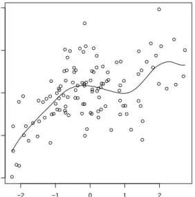
We fit a partially-linear single-index model Y = η(Z⊤α) +X⊤β to the data and choose the bandwidth by generalized cross-validation. We use the scaled Lasso to fit this high-dimensional model and obtain an active set containing 16 variables, including 5 components ofα. The fit of the semiparametric part of the model is shown in Figure 4, showing a clear need of the nonpara-metrically estimated functionη as opposed to using an identity function as in the linear model. The corresponding value of R-squared is 0.72. We apply our method for constructing confidence intervals and find 11 significant variables at a 5% significance level, of which 5 variables are components of α, see Table 5.
−2 −1 0 1 2 −2 −1 0 1 2
Figure 4: Scatterplot of the estimate Z⊤αˆ of the index versus Y −X⊤βˆ. The solid line is the estimate ˆη(Z⊤α,ˆ ξˆ) of η(Z⊤α).
Figure 5(a) we can observe two opposite cases: α16 (VAR27) is selected by the Lasso but is
not significant at a 95% confidence level, while α58 (VAR120) is set to 0 by the Lasso, but
after correction, is shown to be significantly different from zero. The main advantage of our methodology is precisely this ability to take the uncertainty associated with the selection of the zero components into account. In Figure 5(b) we highlight such a variable selected by the Lasso and significant at the 5% level. The same kind of observations can be drawn from Table 5.
(a) (b) −1.0 −0.5 0.0 0.5 components of α 20 40 60 80 −0.4 −0.2 0.0 0.2 0.4 components of β 20 40 60 80 100
Figure 5: Penalized estimator and 95% univariate confidence intervals for the parameters of the PLSIM. (a) Components of α and (b) components of β. Some cases are highlighted and discussed in the text: α16(VAR27), α58 (VAR120) andβ77 (VAR 153).
8
Discussion
We have shown that the desparsifying procedure has its benefits too for the partially linear single-index models. In general, we would recommend using the here proposed confidence intervals and their hypothesis testing equivalents, rather than working with the active sets of selected coefficients only. The simulations and data analysis have illustrated that the set of coefficients set to zero cannot be completely ignored as some of those values might better not have been set to zero. The consistency of selection is an asymptotic property, and comes with selection uncertainty as any model selection method does.
While we concentrated on models with a single index, the method readily extends to multiple indices of the form η(Z1⊤α1, . . . , Zd⊤αd). The single-index model takes d= 1. Due to the curse
of dimensionality, it would be advised to take reasonably low values of d(such as two or three) for efficient estimation.
It is of interest to extend these techniques to generalized partially linear single-index or multiple index models (see Carroll et al. (1997)). It is expected that a combination of the presented theory of this paper combined with the methods of Section 3 of van de Geer et al. (2014) leads to the expected results.
The steps we took to study the effect of a nonparametrically estimated function in the partially linear single-index model, is expected to open the way towards desparsifying methods in other nonparametric and semiparametric models as well. Such issues are beyond the scope of the current paper.
9
Proofs
We define R(α, β) = nPnρ˙ξ and use the same penalty parameter λ for both model parts to
result in a penalty function pλ(α, β). With more notational complexity, the same steps of
the proof hold for different penalty parameters for α and β. The penalized estimator is ˆξ = ( ˆα,βˆ) = arg min{Q(α, β) +pλ(α, β)} and in this notation the desparsified estimator is ˆξdesp =
ˆ
ξ+n−1ΘˆR( ˆα,βˆ).We use the following lemma’s.
Lemma 1. Under the conditions (C1) to (C6)(ii) we have
sup z,α ηˆ(z⊤α;α,βˆ)−η(z⊤α0)=OP{(nh/lnn)−1/2}, (10) sup z,α ηˆ′(z⊤α;α,βˆ)−η′(z⊤α0)=OP{(nh31/lnn)−1/2}. (11)
Proof of Lemma 1. We first show (10). Using lemma A.4 from Wang et al. (2010), it holds that sup
z,α
ηˆ(z⊤α;α, β0)−η(z⊤α0)=OP{(nh/lnn)−1/2}.
Hence we only need to show that sup
z,α |
ˆ
η(z⊤α;α,βˆ)−ηˆ(z⊤α;α, β0)|=OP{(nh/lnn)−1/2}.
Using the equivalent kernel notation for local linear estimators (see Fan and Gijbels (1996), Sec. 3.2.2) with kernel functionsWn,j it suffices to show that
sup z,α | n ∑ j=1 Wnj(Z⊤α, α)Xj⊤( ˆβ−β0)|=OP{(nh/lnn)−1/2}.
Using (C4) and (C6)(ii), and since ∑nj=1Wnj(Z⊤α, α)Xj⊤( ˆβ−β0) is the local linear estimator
using the one-dimensional observationsXj⊤( ˆβ−β0),j= 1, . . . , n, it satisfies the known rates for
one-dimensional smoothing, which proves (10). The second part of the lemma for the estimation of the derivative curve can be shown similarly by using that nh51 is bounded.
Lemma 2. Under the conditions of Theorem 1 we have for each j∈ {1, . . . , p+q} n ∑ i=1 ˆ Θ⊤j,1Zi{ηˆ′(Zi⊤αˆ; ˆξ)−η′(Zi⊤α0)}=oP( √ n).
where Θˆ⊤j,1 is the vector formed by the first p components ofΘˆj•.
Proof of lemma 2. Similarly to (A.22) of Wang et al. (2010), we can show that
n ∑ i=1 ˆ Θ⊤j,1Zi{ηˆ′(Zi⊤αˆ; ˆα, β0)−η′(Zi⊤α0)}=oP( √ n).
It remains to show that∑ni=1Θˆ⊤j,1Zi{ηˆ′(Zi⊤αˆ; ˆα, β0)−ηˆ′(Zi⊤αˆ; ˆα,βˆ)}=oP( √ n) or equivalently that ∑ni=1Θˆ⊤j,1Zi ∑n k=1fWnk(Zi⊤α, α)Xk⊤( ˆβ −β0) = oP( √
n), with fWnk the equivalent kernel
notation for the estimation of the derivative curve. Using condition (C7), the convergence in distribution of the one-dimensional estimator X⊤( ˆβ −β0) and the moment condition on the
equivalent kernel (see Fan and Gijbels (1996), eq. (3.12)), the lemma is proven.
Proof of theorem 1. We rewrite ˆ ξdesp−ξ0 = ˆξ−ξ0+n1Θˆ ∑n i=1{Yi−ηˆ(Zi⊤αˆ; ˆα,βˆ)−Xi⊤βˆ} [ Ziηˆ′(Zi⊤αˆ; ˆα,βˆ) Xi ] = ˆξ−ξ0+n1Θˆ{R1( ˆα,βˆ) +R2( ˆα,βˆ)−R3( ˆα,βˆ)−R4( ˆα,βˆ)−R5( ˆα,βˆ)−R6( ˆα,βˆ)} with R1( ˆα,βˆ) = n ∑ i=1 [ ˜ Ziη′(Zi⊤α0) ˜ Xi ] ϵi, R2( ˆα,βˆ) = n ∑ i=1 [ Zi{ηˆ′(Zi⊤α,ˆ α,ˆ βˆ)−η′(Zi⊤α0)} 0 ] ϵi, R3( ˆα,βˆ) = n ∑ i=1 [ Ziη′(Zi⊤α0) Xi ] {ηˆ(Zi⊤α,ˆ α,ˆ βˆ)−ηˆ(Zi⊤α0, α0, β0) +Xi⊤( ˆβ−β0)}, R4( ˆα,βˆ) = n ∑ i=1 [[ Ziη′(Zi⊤α0) Xi ] { ˆ η(Zi⊤α0, α0, β0)−η(Zi⊤α0) } − [ E[Z|Zi⊤α0]η′(Zi⊤α0) E[Xi|Zi⊤α0] ] ϵi ] , R5( ˆα,βˆ) = n ∑ i=1 [ Zi{ηˆ(Zi⊤α,ˆ α,ˆ βˆ)−η(Zi⊤α0)}{ηˆ′(Zi⊤α,ˆ α,ˆ βˆ)−η′(Zi⊤α0)} 0 ] , R6( ˆα,βˆ) = n ∑ i=1 [ Zi{ηˆ′(Zi⊤α,ˆ α,ˆ βˆ)−η′(Zi⊤α0)} 0 ] Xi⊤( ˆβ−β0).
We show that (i) ˆΘRk( ˆα,βˆ) =oP( √
n) for k∈ {2,4,5} and that
n( ˆξ−ξ0)−ΘˆR3( ˆα,βˆ)−ΘˆR6( ˆα,βˆ) =oP( √
This will imply that√n( ˆξdesp−ξ 0) = √1nΘˆ n ∑ i=1 [ ˜ Ziη′(Zi⊤α0) ˜ Xi ]
ϵi+oP(1) and prove the first part
of the theorem.
Using Lemma 2, it is straightforward to show that ˆΘR2( ˆα,βˆ) is oP( √
n). Using Lemma 1 and conditions (C4) and (C7), we have that
ˆ
Θ⊤j R5( ˆα,βˆ)≤c{nh/ln(n)}−1/2{nh31/ln(n)}−1/2 =oP( √
n),
for each component j, which implies that ˆΘR5( ˆα,βˆ) =oP( √ n). To show (12), we write n( ˆξj −ξj0)−Θˆ⊤j R3( ˆα,βˆ)−Θˆ⊤jR6( ˆα,βˆ) =n e⊤j −Θˆ⊤j 1 n n ∑ i=1 [ Ziη′(Zi⊤α0) Xi ]⊗2 ( ˆξ−ξ0) −Θˆ⊤ j n ∑ i=1 [ Ziη′(Zi⊤α0) Xi ] {ηˆ(Zi⊤α,ˆ α,ˆ βˆ)−ηˆ(Zi⊤α,ˆ α, βˆ 0)} −Θˆ⊤ j n ∑ i=1 [ Ziη′(Zi⊤α0) Xi ] {ηˆ′(Zi⊤α,¯ α, β¯ 0)−η′(Zi⊤α0)}Zi⊤( ˆα−α0)−Θˆ⊤jR6( ˆα,βˆ) = R31−R32−R33−Θˆ⊤j R6( ˆα,βˆ).
We treatR31 and ˆΘ⊤jR6( ˆα,βˆ) together. Using conditions (C6)(iii), (C8) and (C9), we have that
n e⊤j −Θˆ⊤j 1 n n ∑ i=1 [ Ziηˆ′(Zi⊤αˆ; ˆα,βˆ) Xi ]⊗2 ( ˆξ−ξ0) =oP( √ n).
It is thus sufficient to show that ˆ Θ⊤j n ∑ i=1 [ Ziηˆ′(Zi⊤αˆ; ˆα,βˆ) Xi ]⊗2 − [ Ziη′(Zi⊤α0) Xi ]⊗2 ( ˆξ−ξ0)−Θˆj⊤R6( ˆα,βˆ) =oP( √ n) (13) to prove that R31−Θˆ⊤j R6( ˆα,βˆ) = oP( √ n). Writing ˆΘ⊤j = ( ˆΘ⊤j,1,Θˆ⊤j,2) and ˆξ−ξ0 = [ ˆ α−α0 ˆ β−β0 ] , (13) can be decomposed as ˆ Θ⊤j,1 n ∑ i=1 Zi{ηˆ′(Zi⊤αˆ; ˆα,βˆ)2−η′(Zi⊤α0)2}Zi⊤( ˆα−α0) + Θˆ⊤j,2 n ∑ i=1 Xi{ηˆ′(Zi⊤αˆ; ˆα,βˆ)−η′(Zi⊤α0)}Zi⊤( ˆα−α0) + Θˆ⊤j,1 n ∑ i=1 Zi{ηˆ′(Zi⊤αˆ; ˆα,βˆ)−η′(Zi⊤α0)}Xi⊤( ˆβ−β0) − Θˆ⊤ j,1 n ∑ i=1 Zi{ηˆ′(Zi⊤αˆ; ˆα,βˆ)−η′(Zi⊤α0)}Xi⊤( ˆβ−β0).
The last two elements sum up to zero and the first two elements are bothoP( √
n) by Lemma 1 and condition (C6)(i). We thus have R31−Θˆ⊤j R6( ˆα,βˆ) =oP(√n). Showing that R32 and R33
areoP( √
n) will imply thatn( ˆξ−ξ0)−Θˆ⊤j R3( ˆα,βˆ)−Θˆ⊤j R6( ˆα,βˆ) =oP( √ n). For R32, using ˆη(t;α, β) = ∑n j=1Wnj(t, α)(Yj −Xj⊤β), we obtain R32= ˆΘ⊤j n ∑ i=1 [ Ziη′(Zi⊤α0) Xi ] n ∑ j=1 Wnj(Zi⊤α,ˆ αˆ)Xj⊤( ˆβ−β0).
Now, given that∑nj=1Wnj(Zi⊤α,ˆ αˆ)Xj⊤( ˆβ−β0) =Xi⊤( ˆβ−β0) +O(h2), we haveR32=o(n1/2) +
O(nh2) =o(n1/2) by conditions (C4), (C6)(ii) and (C7).
Showing that R33 is oP(√n) is straightforward using Lemma 1, condition (C6)(ii) and the fact
that ¯α is betweenα0 and ˆα.
It remains now to show that ˆΘR4( ˆα,βˆ) = oP(√n) to obtain the asymptotic distribution of √ n( ˆξdesp−ξ0). We write ˆΘR4( ˆα,βˆ) =R4a+R4b with R4a = n ∑ i=1 ˆ Θ⊤j,1η′(Zi⊤α0) [ Zi{ηˆ(Zi⊤α0, α0, β0)−η(Zi⊤α0)} −E[Z|Zi⊤α0]ϵi ] , R4b = n ∑ i=1 ˆ Θ⊤j,2 [ Xi{ηˆ(Zi⊤α0, α0, β0)−η(Zi⊤α0)} −E[X|Zi⊤α0]ϵi ] .
We only show that R4a = oP( √
n), the treatment of R4b is similar. We prove that the mean
and the variance of n−1/2R4a tend to 0. Using E[ˆη(Zi⊤α0, α0, β0)−η(Zi⊤α0)] =O(h2) and the
conditions (C2) and (C7), we have E[n−1/2R4a]≤n−1/2n∥Θˆ⊤j,1Z∥∞sup|η′(Ziα0)|ch2 ≤cn1/2h2
which tends to 0 by condition (C4).
Regarding the variance ofn−1/2R4a, using condition (C7) and lemmas A.2 and A.3 of Wang et al.
(2010), we obtain n−1E[R24a] ≤ cn−1 n ∑ i=1 E [{ ˆ Θ⊤j,1{ n ∑ k=1 Wni(Zk⊤α0, α0)η′(Zk⊤α0)Zk−η′(Zi⊤α0)E[Z|Zi⊤α0] }}2] + n ∑ i=1 E [ ( ˆΘ⊤j,1Zi)2η′(Zi⊤α0)2 {∑n j=1 Wnj(Zi⊤α0, α0)η(Zj⊤α0)−η(Zi⊤α0) )2} ≤ c(nh)−1+c√h+cnh4,
which tends to 0 by (C4) and Lemma A.2 of Wang et al. (2010). This proves that ˆΘR4( ˆα,βˆ) =
oP(√n). Further, it follows that √ n( ˆξdesp−ξ0) = 1 √ n ˆ Θ n ∑ i=1 [ ˜ Ziη′(Zi⊤α0) ˜ Xi ] ϵi+op(1).
Using Lemma 1 and condition (C7), it is straightforward to show that we have a consistent estimator of the variance of √n( ˆξdesp−ξ0). Thus,
ˆ Θ⊤j 1 n n ∑ i=1 [ ˜ Ziη′(Zi⊤α0) ˜ Xi ]⊗2 ˆ Θk−Θˆ⊤j 1 n n ∑ i=1 [ ˜ Ziηˆ′(Zi⊤αˆ; ˆα,βˆ) ˜ Xi ]⊗2 ˆ Θk=o(1).
Acknowledgements
The authors thank the reviewers for their constructive comments. We acknowledge the support of the Fund for Scientific Research Flanders, KU Leuven grant GOA/12/14 and of the IAP Research Network P7/06 of the Belgian Science Policy. The computational resources and services used in this work were provided by the VSC (Flemish Supercomputer Center), funded by the Hercules Foundation and the Flemish Government - department EWI.
References
Carroll, R. J., Fan, J., Gijbels, I., Wand, M. P., 1997. Generalized partially linear single-index models. Journal of the American Statistical Association 92 (438), 477–489.
URLhttp://dx.doi.org/10.1080/01621459.1997.10474001
Chatterjee, A., Lahiri, S. N., 06 2013. Rates of convergence of the adaptive lasso estimators to the oracle distribution and higher order refinements by the bootstrap. Ann. Statist. 41 (3), 1232–1259.
URLhttp://dx.doi.org/10.1214/13-AOS1106
Efron, B., Hastie, T., Johnstone, I., Tibshirani, R., 04 2004. Least angle regression. Ann. Statist. 32 (2), 407–499.
URLhttp://dx.doi.org/10.1214/009053604000000067
Fan, J., Gijbels, I., 1996. Local Polynomial Modelling and its Applications. Vol. 66. CRC Press. Fan, J., Li, R., 2001. Variable selection via nonconcave penalized likelihood and its oracle
prop-erties. Journal of the American Statistical Association 96 (456), 1348–1360. URLhttp://dx.doi.org/10.1198/016214501753382273
Hjort, N. L., Claeskens, G., 2003. Frequentist model average estimators. Journal of the American Statistical Association 98, 879–899.
URLhttp://dx.doi.org/10.1198/016214502388618861
Huang, J., Horowitz, J. L., Wei, F., 08 2010. Variable selection in nonparametric additive models. Ann. Statist. 38 (4), 2282–2313.
URLhttp://dx.doi.org/10.1214/09-AOS781
Huang, J., Ma, S., Zhang, C.-H., 2008. Adaptive lasso for sparse high-dimensional regression models. Statistica Sinica 18 (4), 1603.
URLhttp://www3.stat.sinica.edu.tw/statistica/j18n4/j18n420/j18n420.html Javanmard, A., Montanari, A., 2014. Confidence intervals and hypothesis testing for
high-dimensional regression. Journal of Machine Learning Research 15 (1), 2869–2909. URLhttp://dl.acm.org/citation.cfm?id=2697057
Kabaila, P., 2009. The coverage properties of confidence regions after model selection. Interna-tional Statistical Review 77 (3), 405–414.
URLhttp://dx.doi.org/10.1111/j.1751-5823.2009.00089.x
Leeb, H., P¨otscher, B. M., Ewald, K., 05 2015. On various confidence intervals post-model-selection. Statistical Science 30 (2), 216–227.
URLhttp://dx.doi.org/10.1214/14-STS507
Li, X., Zhao, T., Wang, L., Yuan, X., Liu, H., 2014. flare: Family of Lasso Regression. R package version 1.2.0.
URLhttp://CRAN.R-project.org/package=flare
Liang, H., Liu, X., Li, R., Tsai, C.-L., 12 2010. Estimation and testing for partially linear single-index models. Ann. Statist. 38 (6), 3811–3836.
URLhttp://dx.doi.org/10.1214/10-AOS835
Lockhart, R., Taylor, J., Tibshirani, R. J., Tibshirani, R., 04 2014. A significance test for the lasso. The Annals of Statistics 42 (2), 413–468.
URLhttp://dx.doi.org/10.1214/13-AOS1175
Lu, J., Kolar, M., Liu, H., 2015. Post-regularization confidence bands for high dimensional nonparametric models with local sparsity. arXiv preprint arXiv:1503.02978.
URLhttp://arxiv.org/pdf/1503.02978.pdf
Ma, Y., Zhu, L., 2013. Doubly robust and efficient estimators for heteroscedastic partially linear single-index models allowing high dimensional covariates. Journal of the Royal Statistical Society: Series B (Statistical Methodology) 75 (2), 305–322.
URLhttp://dx.doi.org/10.1111/j.1467-9868.2012.01040.x
Meinshausen, N., Buhlmann, P., 06 2006. High-dimensional graphs and variable selection with the lasso. Ann. Statist. 34 (3), 1436–1462.
URLhttp://dx.doi.org/10.1214/009053606000000281