Procedia Economics and Finance 24 ( 2015 ) 491 – 500
2212-5671 © 2015 The Authors. Published by Elsevier B.V. This is an open access article under the CC BY-NC-ND license (http://creativecommons.org/licenses/by-nc-nd/4.0/).
Selection and/or peer-review under responsibility of the Organizing Committee of ICOAE 2015. doi: 10.1016/S2212-5671(15)00616-4
ScienceDirect
International Conference on Applied Economics, ICOAE 2015, 2-4 July 2015, Kazan, Russia
Univariate GARCH models applied to the JSE/FTSE stock indices
Niel Oberholzer
a*, Pierre Venter
aUniversity of Johannesburg, Department of Finance and Investment Management, Auckland Park, Johannesburg, 2006, South Africa
Abstract
The GARCH(1,1), GJR-GARCH(1,1) and EGARCH(1,1) models will be used to analyse changes in the daily volatility of 5 indices on the Johannesburg Stock Exchange. The 2007-2009 financial crisis was explored to investigate any change in volatility behaviour. Results obtained for the full period of study, 2002 until end 2014, GJR-GARCH was the best fitting model for all the indices except for the JSE/FTSE Top 40 Index. During the financial crisis the GJR-GARCH was the best fitting model for all indices except for the JSE/FTSE Fledgling Index (J204) where EGARCH was the best fitting model.
© 2015 The Authors. Published by Elsevier B.V.
Selection and/or peer-review under responsibility of the Organizing Committee of ICOAE 2015.
Keywords: GARCH (1,1); GJR-GARC(1,1); EGARCH(1,1); Rand; JSE; JSE/FTSE All Share Index (J203); JSE/FTSE Top 40 Index (J200); JSE/FTSE Small Cap Index (J202), JSE/FTSE Mid Cap Index (J201); JSE/FTSE Fledgling Index (J204)
1. Introduction
The history of the South African financial market has always been a market that has been exposed to numerous periods of normal and abnormal volatility. These periods of volatility were not always related to international market contagion but also related to political, economic and financial sanctions. The South African financial market history can be divided into three distinct time periods.
The first period was the period prior to 1985. The end of this period was signalled by the declaration of the debt moratorium by the then South African government in September 1985. The declaration of the debt moratorium signalled the start of the second period in the history of the South African financial markets. The second period was highlighted by the re-introduction of the Financial Rand (ZAL), and the introduction of trade and investment sanction against South African by foreign governments and investors.
* Corresponding author. Tel.: +27-11-559-3483.
E-mail address: nielo@uj.ac.za
© 2015 The Authors. Published by Elsevier B.V. This is an open access article under the CC BY-NC-ND license (http://creativecommons.org/licenses/by-nc-nd/4.0/).
There were three important events that signalled the end of the second period, which started after the first democratic election on 27 April 1994. The first of these events occurred four years before the first election on 11 February 1990 when Nelson Mandela was released by the then national party government. The second was the commencement of the Convention for a Democratic South Africa (CODESA). The third event was the first democratic election on 27 April 1994 which signalled a full transition to democracy and economic independence when the South African Financial Rand (ZAL) was abolished on 13 March 1995 (van der Merwe [19], Aron and Elbadawi [4]).
During these periods investment inflow in the form of foreign direct investment, bond and equity investments were strictly controlled and regulated by the monetary authorities. In 1994 the Johannesburg Stock Exchange (JSE)
followed the example set by the monetary authorities’ by introducing a relaxation of investment controls, and
introduced important regulatory and operational changes.
Since 1994 the South Africa investment market, both foreign and local has become more integrated with international markets, for example the 2007-2009 financial crisis. Apart from the 2007-2009 financial crisis, factors both political and investment related, influenced the South African equity market, for example the investment downgrade of South Africa from investment grade to just above junk bond status.
All these factors resulted in a change in volatility which in turn influenced the forward looking risk and return perception of investors both local and foreign. In this paper three different models namely, GARCH(1,1) (Bollerslev [6]), GJR-GARC(1,1) (Glosten et al. [10]) and EGARCH(1,1) (Nelson [13]), will be used to measure market reaction to the deviations in volatility persistence. In order to investigate the market reaction the following JSE indices will be evaluated: JSE/FTSE All Share Index (J203), JSE/FTSE Top 40 Index (J200), JSE/FTSE Small Cap Index (J202), JSE/FTSE Mid Cap Index (J201) and the JSE/FTSE Fledgling Index (J204). The Akaike information criterion (AIC) [1] and Schwarz information criterion (SIC) [17] will be used to determine the best fitting GARCH model.
The remainder of the paper is structured as follows; part 2 provides a brief review of current literature. Part 3 discusses the methodology and explanation of the data. Part 4 shows the results and interpretation of the findings. Part 5, discusses the conclusion of the study.
2. Literature review
The modelling and understanding of volatility in equity markets is of critical importance in determining of the cost of capital, the evaluation of investment and leveraging decisions (Angabini and Wasiuzzaman [2], Angabini and Wasiuzzaman [3]). Drastic changes in volatility influence the decision making process of risk-averse investors (Premaratne and Balasubramanyan [16]).
When a financial crisis happens like in 2007-2009 the value and parity conditions that occurred, is lost. The impact of a financial crisis is highlighted by the integration of national and international economies (Karunanayake et al. [11]). The subsequent increase in volatility, capital flight of marginal investments, increase in interest rate risk, fears of recession and a reduction in investments are different across emerging markets and developed markets (Tabajara et al. [18]).
The impact and forecasting of volatility resulting from a financial crisis and the different models used is a well-researched field. In a review of financial literature conducted on 93 published and working papers, Poon and Granger [15] provides an in-depth analysis of data via different models used for volatility forecasting. The authors concluded that the GARCH family type models deliver superior forecasting. According to Poon and Granger [15] the GARCH family type of models factors in the more pronounced effect of a negative shock to volatility than a positive shock of the same magnitude.
Brailsford and Faff [7] in their study on Australian equity index data concluded that the GJR-GARCH, as defined by Glosten et al. [10], delivers superior results in the forecasting on volatility. Similar results were obtained by Engle and Ng [9] in their study on Japanese daily stock returns.
Angabini and Wasiuzzaman [2] investigated the impact of the 2007-2009 financial crisis on the Malaysian stock market. The authors compared the results obtained with the persistence of volatility after the Asian Crisis. The findings indicated that there is a major increase in volatility with a small increase in the leverage effect but stated there is a small decrease in the volatility persistence. The study was conducted using GARCH, GJR-GARC and EGARCH.
However, Tabajara et al. [18] uses GARCH, EGARCH and GJR-GARCH models to investigate the impact of volatility on BRIC countries capital markets during the 2007-2009 financial crisis. The authors find that there is less persistence to volatility shocks, less asymmetry and quicker reaction in the market to volatility.
In a study covering the period 2 January 2008 until 11 February 2013, Atoi [4] uses ARCH class models to investigate the effect of news on the volatility in the Nigerian stock market. Atoi [4] results indicate the presence of a leverage effect implying that bad news has a greater impact on volatility than good news.
3. Data and Methodology
The data set used in the study was 3326 daily closing values for the JSE/FTSE Top 40 Index (J200), JSE/FTSE Mid Cap Index (J201), JSE/FTSE Small Cap Index (J202), JSE/FTSE All Share Index (J203) and JSE/FTSE Fledgling Index (J204) covering the period January 2002 to end February 2014. The data set was divided into three sub data sets. This was done to explore any changes in the volatility persistence during the 2007-2009 financial crisis. The first subset covered the full period from 2002 until 2014.The second from 2002 until 2006 and the last from 2002 until 2009. Data was obtained from Reuters Eikon. The data set for each index was analysed by using GARCH, GJR-GARCH and EGARCH models.
The GARCH allows the conditional variance to be used dependent upon its own lags. Brooks [8] specify the model as:
2 2
1 1
t t
V Z DP EV [1]
Where σ equals the estimated conditional variance for one-period ahead based on any past information that is relevant (Brooks [4]). The GJR-GARCH model captures the asymmetric effects of positive and negative random shocks in the market (Neokosmidis [14]). The GJR-GARCH model for conditional variance as specified by Brooks [8] was used. The model specifications are:
t t t t t t u u I if u I Otherwise V Z D EV J ® ¯ 2 2 2 2 1 1 1 1 1 1 1 0 [2]
The leverage effect in the GJR-GARC model is captured by the positive value of the asymmetry term (γ). The
EGARCH model as defined by Nelson [13] captures asymmetric effects. The asymmetric effect is the leverage effect captured by the EGARCH model in relationship to the impact on volatility of news. The effect captured by the EGARCH relates to the increase in volatility when the underlying equity prices decrease i.e. bad news rather than an increase in prices i.e. good news on a similar level. The leverage effect cannot be clarified by the ARCH and
GARCH models. The model specification of the EGARCH model used as defined by Brooks [8] is: 1 2 2 1 1 2 2 1 1 2 ln ln t t t t t u u V Z E V J D S V V ª º « » « » ¬ ¼ [3]
The data analysis and results section will be arranged as follows: descriptive statistics, unit root testing, ARCH LM test, GARCH models and finally diagnostic testing. The AIC and SIC were used to test the relative quality of each of the statistical models relative to one another.
4. Empirical Results
The variables included are not normally distributed. All of the variables are slightly negatively skewed. The kurtosis in each case is greater than 3, which is an indication of leptokurtosis as indicated in Table 1.
Table 1. Data analysis for the period 2002 to end 2006
J203 J200 J201 J202 J204 Mean 0.0007 0.0006 0.0011 0.0012 0.0013 Median 0.0009 0.0010 0.0012 0.0015 0.0013 Maximum 0.0492 0.0545 0.0296 0.0179 0.0317 Minimum -0.0670 -0.0713 -0.0399 -0.0395 -0.0256 Std. Dev. 0.0110 0.0121 0.0064 0.0053 0.0059 Skewness -0.1578 -0.0943 -0.8045 -1.2268 -0.2310 Kurtosis 5.2800 5.1347 7.5282 9.6703 5.4843 Jarque-Bera 273.7422 237.2897 1193.1480 2609.8300 329.8955 Sum 0.8482 0.7825 1.3067 1.4795 1.6642 Sum Sq. Dev. 0.1501 0.1804 0.0505 0.0344 0.0433 Observations 1240 1240 1240 1240 1240 Sources: Researchers analysis
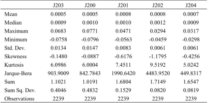
For the period 2002 until the end of 2009, 2239 observations were included. The Jarque-Bera probability test suggests that all the data sets included for each of the JSE/FTSE Indices are not normally distributed. The skewness and kurtosis indicate that the variables are negatively skewed and leptokurtic as shown in Table 2.
Table 2. Data analysis for the period 2002 to end of 2009
J203 J200 J201 J202 J204 Mean 0.0005 0.0005 0.0008 0.0008 0.0007 Median 0.0009 0.0010 0.0010 0.0012 0.0009 Maximum 0.0683 0.0771 0.0471 0.0294 0.0317 Minimum -0.0758 -0.0796 -0.0563 -0.0459 -0.0298 Std. Dev. 0.0134 0.0147 0.0083 0.0061 0.0061 Skewness -0.1480 -0.0887 -0.6176 -1.1795 -0.4256 Kurtosis 6.0986 6.0004 7.4511 9.5192 5.0242 Jarque-Bera 903.9009 842.7843 1990.6420 4483.9520 449.8317 Sum 1.1021 1.0191 1.6804 1.7149 1.6547 Sum Sq. Dev. 0.4046 0.4832 0.1529 0.0820 0.0819 Observations 2239 2239 2239 2239 2239 Sources: Researchers analysis
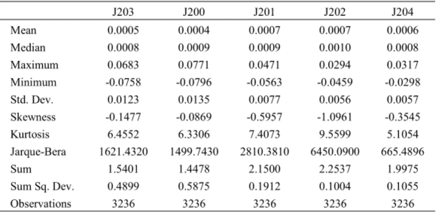
For the full period 3326 observations are included. The mean is close to zero, as indicated in Table 3, which is consistent with what we expect. The variables are not normally distributed and the skewness and kurtosis suggest that the variables are negatively skewed and leptokurtic.
Table 3. Data analysis for the period 2002 to end of 2014
J203 J200 J201 J202 J204 Mean 0.0005 0.0004 0.0007 0.0007 0.0006 Median 0.0008 0.0009 0.0009 0.0010 0.0008 Maximum 0.0683 0.0771 0.0471 0.0294 0.0317 Minimum -0.0758 -0.0796 -0.0563 -0.0459 -0.0298 Std. Dev. 0.0123 0.0135 0.0077 0.0056 0.0057 Skewness -0.1477 -0.0869 -0.5957 -1.0961 -0.3545 Kurtosis 6.4552 6.3306 7.4073 9.5599 5.1054 Jarque-Bera 1621.4320 1499.7430 2810.3810 6450.0900 665.4896 Sum 1.5401 1.4478 2.1500 2.2537 1.9975 Sum Sq. Dev. 0.4899 0.5875 0.1912 0.1004 0.1055 Observations 3236 3236 3236 3236 3236 Sources:Researchers analysis
The results obtained indicate that there is volatility clustering. The volatility clustering suggests that returns, positive or negative, of a large magnitude are usually followed by large returns. In addition, smaller returns usually lead to small returns (Brooks [8]). Furthermore, it is also clear that there was a substantial increase in volatility of all the JSE/FTSE Indices during the financial crisis. This corresponds with results obtained by Angabini and Wasiuzzaman [3] and Atoi [5].
Table 4 confirms that all the variables included are stationary at a level of one percent significance. This is required to be true in order to estimate the GARCH family models in this study.
Table 4. Data analysis for the period 2002 to end of 2014
J203 J200 J201 J202 J204 ADF -55.2402*** -55.9961*** -47.5254*** -26.4623*** -19.2437*** ADF with intercept -55.3107*** -56.0472*** -47.8194*** -27.0095*** -19.7184*** ADF with intercept and trend -55.3027*** -56.0397*** -47.8241*** -27.0363*** -19.8585*** PP -55.3944*** -56.3062*** -48.0125*** -51.9186*** -63.1086*** PP with intercept -55.5058*** -56.4604*** -47.8883*** -50.7696*** -61.5776*** PP with intercept and trend -55.4972*** -56.4530*** -47.8855*** -50.7160*** -61.2408*** *(**) [***]: Statistically significant at a 10(5)[1] % level
Sources: Researchers analysis
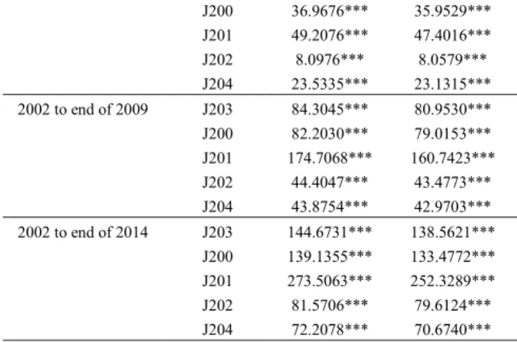
The ARCH-LM-test, as indicated in Table 5, of all the variables included for all the periods are statistically significant at a one percent level of significance. This indicates that there is evidence of ARCH effects. Hence, we can proceed to estimate the GARCH family models.
Table 5. ARCH LM test
Time Period Return Data F-statistic Obs*R-squared 2002 to end of 2006 J203 39.2489*** 38.1034***
J200 36.9676*** 35.9529*** J201 49.2076*** 47.4016*** J202 8.0976*** 8.0579*** J204 23.5335*** 23.1315*** 2002 to end of 2009 J203 84.3045*** 80.9530*** J200 82.2030*** 79.0153*** J201 174.7068*** 160.7423*** J202 44.4047*** 43.4773*** J204 43.8754*** 42.9703*** 2002 to end of 2014 J203 144.6731*** 138.5621*** J200 139.1355*** 133.4772*** J201 273.5063*** 252.3289*** J202 81.5706*** 79.6124*** J204 72.2078*** 70.6740*** *(**) [***]: Statistically significant at a 10(5)[1] % level
Sources: Researchers analysis
According to Brooks [8] if the sum of the coefficients of a GARCH model are close to unity (is close to 1), it implies that shocks to the conditional variance will be persistent. With regards to the GJR-GARCH model, in order for a leverage effect to exist, the asymmetry term will be greater than zero. Conventional wisdom among GARCH researchers is that GARCH models are restricted in the sense that the coefficients cannot be negative. Nelson and Cao [13] argue that the non-negativity constraints in the linear GARCH model are too restrictive. The GARCH model imposes the non-negative constraints on the parameters, while there are no restrictions on these parameters in the EGARCH model.
In considering the GARCH family models for the period 2002 until the end of 2006 in Table 6, the AIC and SIC indicate that the GJR-GARCH is the best fit for the JSE/FTSE All Share Index (J203), JSE/FTSE Top 40 Index (J200), JSE/FTSE Mid Cap Index (J201) and the JSE/FTSE Small Cap Index (J202). The asymmetry terms of all the models are positive and statistically significant and of the correct sign, this suggests that the rise in volatility is of a greater magnitude after a large negative shock. The AIC indicates that EGARCH is the model of best fit when it comes to the JSE/FTSE Fledgling Index (J204). Because the asymmetry term is negative, it suggests that negative shocks lead to higher next period conditional variance. However, the SIC indicates that the GARCH model is the best fit. The sum of the coefficients of the GARCH model is 0.9495, this implies that shocks to the conditional variance will be persistent
Table 6. Coefficients of the GARCH type models for the period 2002 to 2006
Model Return Data ߱ ߙ ߚ ߛ AIC SIC GARCH(1,1) J203 1.80E-06 0.0803** 0.9065*** - -6.3143 -6.2978 J200 2.19E-06 0.0779** 0.9086*** - -6.1250 -6.1085 J201 5.32E-06 0.1596*** 0.7030*** - -7.4181 -7.4015 J202 4.41E-06 0.2211*** 0.6374*** - -7.7564 -7.7398 J204 1.73E-06 0.0510*** 0.8986*** - -7.4807 -7.4642 GJR-GARCH(1,1) J203 2.32E-06 0.0073*** 0.9163*** 0.1116*** -6.3361 -6.3155 J200 2.59E-06 0.0038 0.9209*** 0.1133*** -6.1483 -6.1276 J201 5.34E-06 0.0887*** 0.7158*** 0.1022*** -7.4222 -7.4015 J202 4.74E-06 0.1033*** 0.6404*** 0.1723*** -7.7657 -7.7450 J204 1.68E-06 0.0522*** 0.9007*** -0.0036 -7.4792 -7.4585 EGARCH(1,1) J203 -0.3109 0.1206*** 0.9766*** -0.0827*** -6.3330 -6.3123 J200 -0.2952 0.1151*** 0.9773*** -0.0852*** -6.1458 -6.1252
J201 -1.5227 0.2742*** 0.8720*** -0.0718*** -7.4044 -7.3837 J202 -2.4634 0.3760*** 0.7947*** -0.1097*** -7.7582 -7.7375 J204 -0.5984 0.1357*** 0.9519*** -0.0044*** -7.4813 -7.4607 *(**) [***]: Statistically significant at a 10(5)[1] % level
Sources: Researchers analysis
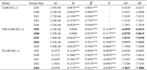
When the periods of the global financial crisis is included in the sample period, the AIC and SIC indicate that the GJR-GARCH model of best fit for all of the JSE indices included with the exception of the JSE/FTSE Fledgling Index (J204). The best fit model for the JSE/FTSE Fledgling Index (J204) is an EGARCH model according to the AIC and SIC. The asymmetry terms of all the relevant models are statistically significant and of the correct sign. This indicates that a large negative shock will provoke a larger increase in the conditional variance as indicated in Table 7.
Table 7. Coefficients of the GARCH type models for the period 2002-2009
Model Return Data ߱ ߙ ߚ ߛ AIC SIC GARCH(1,1) J203 1.87E-06 0.0875*** 0.9031*** - -6.0329 -6.0217 J200 2.24E-06 0.0854*** 0.9050*** - -5.8521 -5.8408 J201 1.73E-06 0.1184*** 0.8562*** - -7.0245 -7.0133 J202 2.58E-06 0.1578*** 0.7797*** - -7.5183 -7.5071 J204 3.35E-06 0.0924*** 0.8204*** - -7.3951 -7.3838 GJR-GARCH(1,1) J203 2.16E-06 0.0030 0.9241*** 0.1159*** -6.0555 -6.0415 J200 2.39E-06 0.0005 0.9274*** 0.1177*** -5.8755 -5.8615 J201 1.98E-06 0.0634*** 0.8587*** 0.0849*** -7.0331 -7.0190 J202 3.23E-06 0.0435** 0.7811*** 0.1498*** -7.5373 -7.5232 J204 4.30E-06 0.0610*** 0.7892*** 0.0666*** -7.3988 -7.3848 EGARCH(1,1) J203 -0.2275 0.1134*** 0.9846*** -0.0850*** -6.0546 -6.0405 J200 -0.2157 0.1086*** 0.9852*** -0.0879*** -5.8755 -5.8614 J201 -0.4543 0.1961*** 0.9693*** -0.0495*** -7.0207 -7.0066 J202 -1.0161 0.2133*** 0.9178*** -0.0893*** -7.5286 -7.5145 J204 -0.9358 0.1719*** 0.9215*** -0.0389*** -7.4027 -7.3886
*(**) [***]: Statistically significant at a 10(5)[1] % level Sources: Researchers analysis
Table 8 displays the GARCH family models for the entire period (2002 until the end of 2014), GJR-GARCH is the best fit model for the JSE/FTSE All Share Index (J203), JSE/FTSE Mid Cap Index (J201) and the JSE/FTSE Small Cap Index (J202), EGARCH is the best fit model when the JSE/FTSE Top 40 Index (J200) is considered. The asymmetry terms of all these models are statistically significant and of the correct sign. This indicates that a negative shock of a large magnitude will lead to a larger increase in the conditional variance when compared to the effect of a positive shock. For the JSE/FTSE Fledgling Index (J204), the AIC indicates that the EGARCH model is the best fit. Although the SIC indicates that the best fit model is the GARCH model. The asymmetry term implies that a large negative shock will provoke a larger increase in the conditional variance. Furthermore, the sum of the coefficients of the GARCH model is close to unity, which suggests that these shocks will be persistent.
Table 8. Coefficients of the GARCH type models for the period 2002-2014
Model Returns Data ɘ Ƚ Ⱦ Ȟ AIC SIC GARCH(1,1) J203 1.57E-06 0.0831*** 0.9070*** - -6.2491 -6.2416
J200 1.88E-06 0.0815*** 0.9085*** - -6.0625 -6.0550 J201 1.67E-06 0.1028*** 0.8669*** - -7.1499 -7.1424
J202 1.91E-06 0.1315*** 0.8084*** - -7.7083 -7.7008 J204 2.22E-06 0.0803*** 0.8514*** - -7.5627 -7.5551 GJR-GARCH(1,1) J203 1.66E-06 -0.0006 0.9262*** 0.1219*** -6.2768 -6.2674 J200 1.89E-06 -0.0036 0.9291*** 0.1247*** -6.0913 -6.0819 J201 1.85E-06 0.0528*** 0.8708*** 0.0757*** -7.1579 -7.1485 J202 2.33E-06 0.0572*** 0.8040*** 0.1076*** -7.7201 -7.7107 J204 2.59E-06 0.0672*** 0.8364*** 0.0301** -7.5633 -7.5539 EGARCH(1,1) J203 -0.2300 0.1143*** 0.9847*** -0.0929*** -6.2765 -6.2671 J200 -0.2205 0.1098*** 0.9850*** -0.0962*** -6.0917 -6.0823 J201 -0.4369 0.1743*** 0.9697*** -0.0487*** -7.1479 -7.1385 J202 -0.8729 0.2110*** 0.9326*** -0.0655*** -7.7118 -7.7024 J204 -0.7395 0.1583*** 0.9405*** -0.0193*** -7.5644 -7.5550
*(**) [***]: Statistically significant at a 10(5)[1] % level Sources: Researchers analysis
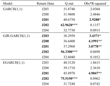
With regards to diagnostic checking (summarised by Tables 9-11), of the best fit models for the period 2002 until the end of 2006, the GJR-GARCH model of the volatility of the JSE/FTSE Small Cap Index (J202) suffers from serial correlation at a one percent level of significance. For the period 2002 until the end of 2009, the EGARCH model of the volatility of the JSE/FTSE Small Cap Index (J202) also suffers from serial correlation at a one percent level of significance. Finally, for the period 2002 until the end of 2014, there is evidence of ARCH effects, at a one percent level of significance, when the GJR-GARCH model is applied to the JSE/FTSE All Share Index (J203); similarly, when the EGARCH model is applied to the JSE/FTSE Top 40 Index (J200).
Table 9.Diagnostic testing of models for period the 2002 to 2006
Model Return Data Q stat Obs*R-squared GARCH(1,1) J203 31.8740 2.0304 J200 31.9600 2.4846 J201 40.6750 2.9288* J202 62.9620*** 0.1157 J204 32.7730 0.0915 GJR-GARCH(1,1) J203 36.2950 3.4371* J200 36.6400 4.1991** J201 37.2960 3.0778** J202 56.3300*** 0.0698 J204 32.6040 0.1012 EGARCH(1,1) J203 40.3120 1.8615 J200 39.1710 2.3610 J201 45.8970 4.9847** J202 75.5150*** 0.0962 J204 31.7240 0.0742 *(**) [***]: Statistically significant at a 10(5)[1] % level
Sources: Researchers analysis
Table 10. Diagnostic testing of models for period 2002 to 2009
Model Return Data Q stat Obs*R-squared GARCH(1,1) J203 33.4370 3.1857*
J200 31.9370 3.4463*
J202 51.3610** 0.0365 J204 33.3420 0.7309 GJR-GARCH(1,1) J203 38.1530 6.1533** J200 38.2450 6.4200** J201 34.5920 2.6217 J202 42.0320 0.0417 J204 39.8510 0.6621 EGARCH(1,1) J203 39.5910 3.7966* J200 38.5110 4.0142** J201 34.5410 4.8161* J202 56.7930*** 0.8369 J204 34.8490 0.1623 *(**) [***]: Statistically significant at a 10(5)[1] % level
Sources: Researchers analysis
Table 11. Diagnostic testing of models for period 2002-2014
Model Returns Data Q stat Obs*R-squared GARCH(1,1) J203 34.8430 4.0620** J200 34.0160 4.7960** J201 33.0910 2.4323 J202 58.4040*** 0.1374 J204 29.2910 0.1713 GJR-GARCH(1,1) J203 40.7690 8.2977*** J200 41.7800 9.2675*** J201 33.2170 2.2317 J202 50.3660* 0.0736 J204 32.1990 0.1772 EGARCH(1,1) J203 42.8880 6.1684** J200 43.0320 7.0624*** J201 34.9470 5.2393** J202 69.2570*** 1.0375 J204 30.3230 0.0888 *(**) [***]: Statistically significant at a 10(5)[1] % level
Sources: Researchers analysis
5. Conclusion
The purpose of this paper was to assess the applicability of three GARCH family type models in the quantifying and forecasting of volatility on the JSE for the 5 major indices for the period 2002 until end 2014. The study period was subdivided into three periods to investigate the impact of volatility resulting from the 2007-2009 financial crisis. For the full period of study, 2002 until end 2014, GJR-GARCH was the best fitting model for all the indices except for the JSE/FTSE Top 40 Index (J200). For the second period where the impact of the financial crisis on the JSE indices was investigated the GJR-GARCH was the best fitting model for all the indices except for the JSE/FTSE Fledgling Index (J204) were EGARCH was the best fitting model in both periods. The results obtained indicate evidence of leverage effects when the GARCH models of the JSE/FTSE All Share Index (J203), JSE/FTSE Top 40 Index (J200), JSE/FTSE Small Cap Index (J202), JSE/FTSE Mid Cap Index (J201) and the JSE/FTSE Fledgling Index (J204) are considered. This suggests that the rise in volatility is of a greater magnitude after a large negative shock, when compared to that of a positive shock.
References
[1] Akaike, H., 1974. A New Look at the Statistical Model Identification. IEEE Transactions on Automatic Control Ac-19, 716-723. [2] Angabini, A., Wasiuzzaman, S., 2011a. GARCH Models and the Financial Crisis-A Study of the Malaysian Stock Market. International Journal of Applied Economics and Finance 5, 226-236.
[3] Angabini, A., Wasiuzzaman, S., 2011b. Impact of the Global Financial Crisis on the Volatility of the Malaysian Stock Market, International Conference on E-business, Management and Economics. Hong Kong, IACSIT Press, Hong Kong.
[4] Aron, J., Elbadawi, I., 1999. Reflections on the South African rand crisis of 1996 and policy consequences. The Berkley Electronic Press. [5] Atoi, N.V., 2014. Testing Volatility in Nigeria Stock Market using GARCH Models. CBN Journal of Applied Statistics 5, 65-93. [6] Bollerslev, T., 1986. Generalised Autoregressive Conditional Hetroskedasticity. Journal of Econometrics 3, 307-327.
[7] Brailsford, T. J., Faff, R.W., 1996. An evaluation of volatility forecasting techniques. Journal of Banking and Finance 20, 419-438. [8] Brooks, C., 2008. Introductory Econometrics for Finance, United Kingdom, University Press, Cambridge.
[9] Engle, R.F., Ng, V.K., 1993. Measuring and testing the impact of news on volatility. Journal of Finance 20, 419-438.
[10] Glosten, L.R., Jagannathan, R., Runkle, D., 1993. On the relation between the expected value and the volatility of the nominal excess return on stocks. Journal of Finance 48, 1779-1801.
[11] Karunanayake, I., Valadkhani, A., O'Brien, M., 2010. The Effects of Financial Crises on International Stock Market Volatility Transmission. School of Economics, University of Wollongong, Australia.
[12] Nelson, D.B., 1991. Conditional Heteroskedasticity in Asset Returns: A New Approach. Econometrica 59, 347-370.
[13] Nelson, D.B., Cao, C.Q., 1992. Inequality constraints in the univariate GARCH model. Journal of Business & Economic Statistics 10, 229-235.
[14] Neokosmidis, I., 2009. Econometric Analysis of realized Volatility: Evidence of Financial Crisis. PhD, Aristotle University of Thessaloniki. [15] Poon, S.H., Granger, C.W.J., 2003. Forecasting Volatility in Financial Markets: A Review. Journal of Economic Literature 41, 478-539. [16] Premaratne, G., Balasubramanyan, L., 2003. Stock market volatility: Examing North America, Europe and Asian. National University of Singapore.
[17] Schwartz, G., 1978. Estimating the Dimension of a Model. The Annals of Statistics 6, 461-464.
[18] Tabajara, P.J., Fabiano, G.L., Luiz, E.G., 2014. Volatility behaviour of BRIC capital markets in the 2008 international financial crisis. African Journal of Business Management 8, 373-381.