Projection Pursuit for Discrete Data
Persi DiaconisDeptartment of Mathematics and Department of Statistics Stanford University Julia Salzman Deptartment of Statistics Stanford University July 3, 2006
1
Introduction
Projection pursuit is an exploratory graphical tool for picturing high dimen-sional data through low dimendimen-sional projections. Introduced by Kruskal (1969), and developed by Friedman and Tukey (1974), the idea is to have the computer select a small family of projections by numerically optimizing an index of “interest”. The original projection indices were ad hoc. In joint work with David Freedman (1984), it was shown that for most data sets, most projections are about the same: approximately normal.
Therefore, interesting projections are those which are far from normal. Peter Huber (1985) found his own version of this: projections are uninfor-mative if they are unstructured or “random”. Thus projections with high entropy are uninformative. For a fixed scale, a distribution having high en-tropy or approximately normality are equivalent. Huber also showed that the Friedman-Tukey index is a measure of non-normality.
The purpose of the present paper is to give a parallel development for data in discrete spaces: collections of binary vectors, rankings or phylo-genetic trees; or sets of graphs. We develop a notion of projection as a partition of the discrete data into blocks. We show that most for most data sets, most projections are close to uniformly partitioned. This suggests that the informative summaries are the ones with splits that are far from uniform. The outline of the paper is as follows. Definitions and first examples are given in Section 2. The ideas lean on classical developments in block designs and give new applications for that theory. A discrete version of the Radon transform along with an inversion theory is presented, determining when a collection of projections loses information. Section 3 gives a data analytic
example in some detail. The data arises from the problem of putting some of Plato’s works in chronological order. Here, discrete projection pursuit leads to the discovery of a striking, easily interpretable structure that does not appear in other analyses of this data (eg. Ahn et al. (2003), Cox and Brandwood (1959), Holmes (2001), Wishart and Leach (1970)). Section 4 proves that for most data sets, most partitions lead to approximately uniform projections. This leads directly to a usable criteria: a projection is interesting if it is far from uniform. The distance to uniformity can be measured by any distance between probabilities, and we consider the well-known total variation, Hellinger and Vasserstein metrics.
The final section gives results for the least uniform projection. Theorem ?? shows that if the class of projections is not too rich, for example, the affine hyperplane in Zk, then for most data sets even the least uniform
partition is close to uniform. If the class of projections contains many sets, then least uniform projections are “structured”. The final theorem attacks the problem of a data analyst finding “structure” in “noise”.
There has been extensive development of projection pursuit for den-sity estimation (Friedman et al. (1984)), regression (Friedman and Stuetzle (1981); Hall (1989)), applications to time series (Donoho (1981)), discrimi-nant analysis (Posse (1992); Polzehl (1995)) and standard multivariate prob-lems such as covariance estimation (Hwang et al. (1995)). This has led to a healthy development captured in the modern implementations (Xgobi, Ggobi). Online documentation for this software is an instructive catalog. We have not attempted to develop our ideas in these directions, but the beginning steps of ridge functions will be found below.
This paper is written in tribute to David Freedman with thanks for his integrity and brilliance.
2
Projections and Radon Transforms
This section introduces our notation and set up for working with discrete data. It defines projection bases, the discrete Radon transform and gives ex-amples with binary data and permutation data. Analysis will be performed on binaryn−tuple data from several works of Plato. LetX be a finite set. LetY be a class of subsets ofX. Letf :X →Rbe a function. The Radon transform off aty ∈ Y is defined by
¯
f(y) =X
x∈Y
The class Y is called a projection base if
|y| is constant fory∈ Y (|y| denotes the cardinality ofY) (2) There is a partitionp1, . . . pj of Y s.t. each pi is a partition ofX(3)
For a partitionp, the numbers ¯f(y)y∈p will be called the projection off
in direction p. The sets in Y may be thought of as “lines” in a geometry. If lines in the same partition are called parallel, then (??) corresponds to the Euclidean axiom: for every point x ∈ X and every line y ∈ Y, there is a unique line y∗ parallel to y such that x ∈ y∗. In the statistics
litera-ture, designs with property (??) are called “resolvable” (See Hedayat et al. (1999) or Constantine (1987) for examples). Assumption (??) guarantees that projections are based on averages over comparable sets.
Consider the following examples:
Example 2.1. X =Zk2 the set of binaryk−tuples. Here is a concrete
exam-ple of a data set with this structure; L. Brandwood classified each sentence of Plato’s Republic according to its last five syllables. These can run from all short (∪) through all long (-). Identifying ∪ with 1 and - with 0, each sentence is associated with a binary 5−tuple. Asx ranges over Z52, let f(x)
denote the proportion of sentences with ending x. The values of f(x) are given in the first column of Table 1.
A second example of data with this structure is the result of grading correct/incorrect in a test withk questions. There are several useful choices ofY given next:
2.1 Projections for data in Zk2 2.1.1 Marginal projections in Zk2
For i= 1,2, . . . k, let yi0 ={x ∈Zk2 : xi = 0}, let yi1 = {x ∈ Zk2 : xi = 1}.
The setsY ={yji},1≤i≤k, j∈ {0,1}form a projection base. In the Plato example, the projections have a simple interpretation as the proportion of sentences with a specific ending in the ith place. Displaying projections
offers no problem here; a single number suffices.
A second natural choice of Y gives second order margins. This is based on sets yabij = {x ∈ Zk2 : xi = a, xj = b},1 ≤ i < j ≤ k, a, b ∈ {0,1}.
In this case, a projection consists of 4 numbers. In the Plato example, the projection along coordinatesi, j gives the proportion of sentences with each
Table 1
Percentage Distribution of Sentence Endings Type of ending Rep. Laws Phil. Pol. Soph. Tim. ∪ ∪ ∪ ∪ ∪ 1.1 2.4 2.5 1.7 2.8 2.4 - ∪ ∪ ∪ ∪ 1.6 3.8 2.8 2.5 3.6 3.9 ∪- ∪ ∪ ∪ 1.7 1.9 2.1 3.1 3.4 6.0 ∪ ∪- ∪ ∪ 1.9 2.6 2.6 2.6 2.6 1.8 ∪ ∪ ∪- ∪ 2.1 3.0 4.0 3.3 2.4 3.4 ∪ ∪ ∪ ∪- 2.0 3.8 4.8 2.9 2.5 3.5 - -∪ ∪ ∪ 2.1 2.7 4.3 3.3 3.3 3.4 - ∪- ∪ ∪ 2.1 1.8 1.5 2.3 4.0 3.4 - ∪ ∪- ∪ 2.8 0.6 0.7 0.4 2.1 1.7 - ∪ ∪ ∪- 4.6 8.8 6.5 4.0 2.3 3.3 ∪- - ∪ ∪ 3.3 3.4 6.7 5.3 3.3 3.4 ∪- ∪- ∪ 2.6 1.0 0.6 0.9 1.6 3.2 ∪- ∪ ∪ - 4.6 1.1 0.7 1.0 3.0 2.7 ∪ ∪- - ∪ 2.6 1.5 3.1 3.1 3.0 3.0 ∪ ∪- ∪ - 4.4 3.0 1.9 3.0 3.0 2.2 ∪ ∪ ∪- - 2.5 5.7 5.4 4.4 5.1 3.9 - - -∪ ∪ 2.9 4.2 5.5 6.9 5.2 3.0 - -∪ - ∪ 3.0 1.4 0.7 2.7 2.6 3.3 - -∪ ∪ - 3.4 1.0 0.4 0.7 2.3 3.3 - ∪- - ∪ 2.0 2.3 1.2 3.4 3.7 3.3 - ∪- ∪- 6.4 2.4 2.8 1.8 2.1 3.0 - ∪ ∪- - 4.2 0.6 0.7 0.8 3.0 2.8 ∪ ∪- - - 2.8 2.9 2.6 4.6 3.4 3.0 ∪- ∪- - 4.2 1.2 1.3 1.0 1.3 3.3 ∪- - ∪- 4.8 8.2 5.3 4.5 4.6 3.0 ∪- - - ∪ 2.4 1.9 5.3 2.5 2.5 2.2 ∪- - - - 3.5 4.1 3.3 3.8 2.9 2.4 - ∪- - - 4.0 3.7 3.3 4.9 3.5 3.0 - -∪ - - 4.1 2.1 2.3 2.1 4.1 6.4 - - -∪ - 4.1 8.8 9.0 6.8 4.7 3.8 - - - -∪ 2.0 3.0 2.9 2.9 2.6 2.2 - - - 4.2 5.2 4.0 4.9 3.4 1.8 no. sentences 3778 3783 958 770 919 762
of the 4 possibles patterns ∪ ∪, ∪ -, - ∪, - - in positions i, j. Table 3 in Section 3 is an example of one method displaying such projections. Section 2 contains an analysis of the data in Table 1 based on these projections. The analysis gives a clear interpretation to a classical way of dating the books of Plato. The analysis is independent of the other examples in this section and can be read at this time.
Here are some examples to show how the structure of f is reflected in ¯
f. If f(x) = δx,x0,f¯(y) = 1 if x0 ∈ y and zero otherwise. If f(x) =
1 2k,
¯
f(y) = |2yk| and hence is constant for all y. As a final example, consider a
fixed, non-zero vector y∗ ∈ Zk
2. Let S be the hyperplane determined by y∗ :S ={x∈Zk2 :x·y= 0 mod 2}. Let
f(x) = 1
2k ifx∈S
0 otherwise An easy computation shows
¯ f(yz0) = 1 ifz=y∗ 1 2 otherwise ¯ f(yz1) = 0 ifz=y∗ 1 2 otherwise
The hyperplane transform is essentially the same as the ordinary Fourier transform on the groupZk2. This is defined by
ˆ
f(x) =X
x
(−1)x·zf(x).
Iff is a probability onZk2, ˆf(z) = 2 ¯f(y0z)−1. The transform ˆf has been
widely used for data analysis of this type of data. See Solomon (1961) or Diaconis (1996 Chapter 11, 1997). The discrete Radon transform with pro-jections onto affine hyperplanes is also used by Ahn, Hofman Cook (2003). 2.1.2 Affine hyperplanes in Zk2
This is one natural way of “filling out” the marginal projections presented above. For z ∈Zk2 and a∈ {0,1}, let yza = {x ∈ Zk2 : x·z = amod 2}.
The collection Y ={ya z}z∈Zk
2, a∈{0,1} forms a projection base. Observe that
when z has a 1 in position i and zeros elsewhere, yza equals the yia of the previous example. The sets inY are the affine hyperplanes inZk2. Similarly,
the affine planes of any dimension form a projection base. An analysis of the Plao data using all affine hyperplanes is in AppendixA.3 below.
2.2 Projections for data in X =Sn, the sets of permutations
of n letters.
Permutation data arises in taste testing, ranking and elections; for example, in presidential elections of the American Psychological Association, members are asked to rank order 5 candidates. Here, for a permutation π, f(π) is taken as the proportion of voters choosing the order π. For background and many examples, see Critchlow (1988), Fligner and Verducci (1993) or Marden (1995).
2.2.1 Partitions based on marginal projections of permutations in Sn.
Let yij ={π ∈ Sn : π(i) = j, 1 ≤i, j ≤n}. These sets form a projection
base. For fixedi, the setsyi1, yi2, . . . yinform a partitionp(i). The projection
in directionp(i) has a natural interpretation in the example: how did people rank candidatei? The projection can be displayed by making a histogram. A second useful choice ofY is based on considering two positions: yijkl= {π ∈ Sn : π(i) = k, π(j) = l} i 6= j, k 6= l. This leads to projections
giving the joint rankings of a fixed pair of candidates in the example. Such projections can be displayed by making a 2-dimensional picture and gray scaling the (i, j) square to correspond to the proportion of voters ranking the pair of candidates in order (i, j). Similarly third and higher order projections can be defined.
2.2.2 Partitions based on subgroups of Sn.
When X is a group such as Sn, the following constructions forY are
avail-able. LetN be a subgroup ofX. The orbits ofN acting onX are the cosets {N y}y∈X, and the distinct orbits partition X. Varying N by conjugation,
{yN y−1}y∈X, gives a projection base forX.
When N is taken as Sn−1 = {π ∈ Sn : π(1) = 1} the projections are
the marginal projections defined above. Taking N as Sn−2 = {π ∈ Sn : π(1) = 1, π(2) = 2} gives the second order margins. An important class of subgroups are the so-called Young subgroups: let λ1 ≤ λ2 ≤ . . . λn be
a partition of n so P
iλi = n. Let Sλ1 ×Sλ2 ×. . .×Sλn be the
permu-tations that permute the first λ1 elements among themselves and the next λ2 elements among themselves, etc. These include the previous examples
and provide enough transforms for an inversion theory, as will be shown below. Display of such projections is not a well studied problem. In the case of a projection corresponding to a Young subgroup, one suggestion is a
1-dimensional histogram using one of the orderings suggested in Chapter 3 of James (1978).
If X =G/H whereGis a group and H is a subgroup and G⊂N ⊂H, withN a subgroup, then the orbits ofN inX are a partition and the orbits of{gN g−1}
g∈G form a partition base. One approach to the display of such
projections is a 2-dimensional histogram using the ordering given by one of the metrics suggested in Chapter 7 of Diaconis (1986).
2.3 Projections for X =Rp: Euclidean data.
Consider data vectors x1, x2, . . . xn ∈Rp. For γ in the p−dimensional unit
sphere, the projection in direction γ is just γ ·x1, . . . , γ ·xn. This is the
classical Radon transform, withY consisting of the affine hyperplanesyγt =
x∈Rp :x·γ =t. For fixed γ these partition the space Rp ast varies, and
the partitions vary as γ varies. In statistical applications, a histogram is made of γ·xi and one varies γ, trying to understand the structure of the p−dimensional data from the varying histograms. This leads to the classical version of projection pursuit considered in the introduction.
2.4 Projections when X is a finite set with n elements, and Y is the class of k− element subsets.
In this example, it is a non-trivial theorem of Baranyai that Y forms a projections base. Details and discussion may be found in Cameron (1976). This example occurs naturally when considering extensions of a given class of partitions. For example, consider the marginal projectionsya
i inZk2 defined
above. These sets all have cardinality |y1a|= 2k−1. It is natural to consider the extension to projections based on the class of all subsets of cardinality 2k−1.
2.5 Uniqueness of Radon Transforms:
We now consider the question: when is f → f¯one to one? A convenient criteria involves the notion of a block design. Let|X |=n. The class of sets Y is a block design with parameters (n, c, k, l) provided
|y|=c for ally∈ Y (4)
each x∈ X is contained ink subsets y (5) each pairx6=x0 is contained in lsubsets y (6)
Affine planes orZk2andksets of annset are block designs. A great many
other examples are discussed in the literature of combinatorial designs. In the statistics literature they are sometimes called balanced incomplete block designs. In the combinatorial literature they are often called 2−designs, or 2−(n, c, l) designs. It is easy to see that the parametersn, c, k, l satisfy
|Y|c = nk (7)
(n−1)l = k(c−1) (8)
Dembroski (1968) and and Lander (1982) are useful references for block designs.
The following result is well known in the theory of designs. We first learned it from Bolker (1987).
Theorem 2.2. If X is a finite set and Y is a block design with |Y| > 1, the the Radon transform f → f¯is one to one, with an explicit inversion formula given by(??) below.
Proof. For anyx, X y:x∈y ¯ f(y) = kf(x) +l X s,s0∈X x6=x0 f(x0) (9) = (k−l)f(x) +lX x∈X f(x) (10) IfP x∈X f(x) = 1, this determinesf as f(x) = 1 k−l X y0x∈y ¯ f(y)− l k−l. (11)
Observe that k > l follows from the assumption that |Y| > 1. When P
x∈X f(x) is not known, it can be recovered by summing both sides of
(??) inx. This gives X x∈X f(x) = c k−l+nl X y∈Y ¯ f(y) and so the inversion formula
f(x) = 1 k−l X y:x∈y ¯ f(y) + lc (k−l)2+nl(k−l) X y∈Y ¯ f(y) (12)
Remarks:
• It is not necessary thatYbe a block design forf → f¯to be one to one. For example, Kung (1979) shows that the Radon transform is one to one whenY consists of the sets of rank iin a matroid. Diaconis and Graham (1985) give examples where the transform is one to one when Y consists of the nearest neighbors in a metric space. For example, when X =Z2k2 and Y consists of the balls of Hamming distance less
than or equal to 1, the transform is one to one, and an explicit inversion theorem is known. WhenX isSn, the symmetric group, andY is unit
balls in the Cayley metric, the transform is one to one if and only if n is in {1,2,4,5,6,8,10,12}. Further work on inversion formulas for functions on finite symmetric spaces is found in Velasquez (1997) and for functions on the torus Zkn in Dedeo and Velasquez (2004).
Fill (1989) discusses invertibility when the Radon transform of f at
x averages over a set of translates of f(x) which has applications to directional data and time series.
• The transform can still be useful and interesting if it is not one to one. For example, the marginal projections in the example above do not capture all aspects of the data but are often the first things to be looked at. In Zk2, if high enough marginal distributions are considered, the
functionf can be completely recovered. In the symmetric group, the projections corresponding to all Young subgroups determinef because they determine it’s Fourier transform. See Diaconis (1986) for details.
3
Data analysis of syllable patterns in the works
of Plato
This section presents a new analysis of data arising from syllable patterns in the works of Plato. The data is given in Table 1. It records, for each of 6 books, the pattern of long (-) and short (∪) syllables among the last 5 syllables in each sentence. It is known that Plato wroteRepublic early and Laws late. Plato also mentions that he changed his rhyming patterns over time. This led Brandwood to collect the data in Table 1.
The other books were written between these but it is not known in what order. The goal of the analysis is to try to order the books. Our approach will be to study the books one at a time, trying to find patterns.
Projection pursuit suggests looking at various partitions of the data, searching for structured partitions which are far from uniform. Using first and second order margins as partitions, a reasonably striking difference be-tweenRepublic andLaws is observed. This suggests a simple, interpretable way of ordering the other books as Republic, Timaeus, Sophist, Politicus, Philebus, Laws.
This agrees with the standard ordering as discussed in Brandwood (1976, pg. XViii) and in Ahn et Al (2003). Other analyses of this data set are in Cox and Brandwood (1959), Atchinson (1970), Wishart and Leach (1970) and Boneva (1971). The last reference contains a history and explanation for the choice of data. The first three analyses all use statistical models. Boneva’s analysis uses a form of scaling. None of the previous analyses seem to have picked up the simple, striking pattern in the data that projection pursuit leads to.
The analysis is presented below, in a somewhat discursive style, in the order it was actually performed: first looking at the Republic, then Laws and finally the other books. In the Appendix, we present a more automated and formal version.
3.1 Republic
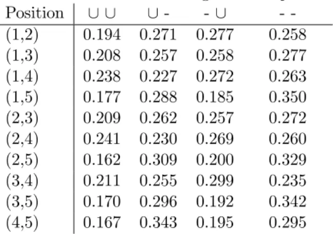
Table 2 shows the first order margins; e.g., the proportion of sentences with ∪in positioni, 1≤i≤5.
Table 2: First order margins for Republic
Position 1 2 3 4 5
Proportion of ∪ 0.465 0.471 0.466 0.511 0.362
Roughly, positions 1-4 are evenly divided between long and short. The last position is clearly different. Table 3 shows the second order margins.
Table 3: Second order margins for Republic Position ∪ ∪ ∪ - - ∪ -(1,2) 0.194 0.271 0.277 0.258 (1,3) 0.208 0.257 0.258 0.277 (1,4) 0.238 0.227 0.272 0.263 (1,5) 0.177 0.288 0.185 0.350 (2,3) 0.209 0.262 0.257 0.272 (2,4) 0.241 0.230 0.269 0.260 (2,5) 0.162 0.309 0.200 0.329 (3,4) 0.211 0.255 0.299 0.235 (3,5) 0.170 0.296 0.192 0.342 (4,5) 0.167 0.343 0.195 0.295
A glance at Table 3 shows that the first order effects are all too visible in the second order margins. For example, the numbers in the first column (∪ ∪) are all “small” while the numbers in the last column are “large”. One simple way of adjusting for the first order structure is to divide each number in Table 3 by the product of the marginal totals. For example, in the first row, .194 would be divided by (.465)(.472) (from Table 2) while .271 would be divided by (.465)(1−.472). The results are shown in Table 4:
Table 4: Adjusted second order margins forRepublic Position ∪ ∪ ∪- - ∪ -(1,2) 0.89 1.10 1.10 0.91 (1,3) 0.96 1.00 1.00 0.97 (1,4) 1.00 1.00 1.00 1.00 (1,5) 1.10 0.97 0.96 1.00 (2,3) 0.95 1.00 1.00 0.96 (2,4) 1.00 1.00 1.00 1.00 (2,5) 0.95 1.00 1.00 0.97 (3,4) 0.89 1.10 1.10 0.90 (3,5) 1.00 1.00 0.99 1.00 (4,5) 0.90 1.10 1.10 0.94
Most of the ratios are close to 1, so a product model is a reasonable first description. The projection pursuit approach suggests that a partition of the data (here a row) is “interesting” if the partition is far from uniform. By eye, looking at Table 4, positions (1,2),(2,3),(3,4),(4,5) are far from being all 1. Observe that these positions are adjacent, as (i, i+ 1).
Next observe that each of the 4 designated rows has a common pattern: the first and last entries are small, the middle two entries are large. Going back to the definitions, this pattern arises from a negative association of adjacent syllables; in theRepublic, adjacent syllables tend to alternate. The pattern in positions (1,3) shows that this cannot be a complete description; after all, if the symbols alternate, the positions two apart should be pos-itively associated, but (1,3) displays negative association. Looking at the other rows of the table, we observe that the size goes big, small, small, big or its opposite, small, big, big, small. This is an artifact. Consider the first row of Table 4. It was formed from 4 proportions that sum to 1: w, x, y, z
say. The 4 adjusted entries are
w (w+x)(w+y) x (w+x)(x+z) y (y+z)(y+w) z (z+y)(z+x). It is easy to show that the first entry is less than 1 if and only if the second is larger than 1, if and only if the third is larger than one if and only if the fourth is less than 1. This means that the first column in Table 4, together with the first order margins, determines the remaining entries. This artifact in no way reflects on the association pattern noted earlier– the most structured rows correspond to adjacent syllables, and adjacent syllables are negatively associated.
3.2 Laws and a comparison with Republic.
The first order margins for Laws are only slightly different from those in Republic:
Table 5: First order margins forLaws
Position 1 2 3 4 5
Proportion of ∪ ∪ 0.477 0.489 0.411 0.599 0.375
The pattern is the same: overall, fewer than half ∪’s; the last position sharply smaller. The similarity between the first order margins inRepublic and Laws suggests that second or higher order margins must be used to order the remaining books. The analog of the first column of Table 4 is given below:
Table 6: Adjusted second order margins forLaws
Positions (1,2) (1,3) (1,4) (1,5) (2,3) (2,4) (2,5) (3,4) (3,5) (4,5) Adjusted∪ ∪ 1.07 1.03 0.92 0.99 1.43 0.97 0.98 1.04 1.09 1.02
The entries above are the proportion of sentences with ∪ ∪in the (i, j) position divided by the product of the marginal proportions.
Again, pairwise adjacent positions are associated, all in the same way. Here, the association is positive, whereas for Republic, the association is negative. This is the striking pattern referred to above. It suggests a method of ranking the of the books: compare the sign pattern or actual ratios of the adjusted second order margins of other books withRepublic andLaws.
For definiteness, the sum of absolute deviations between second order margins over all 10 positions will be used. This is carried out data analyti-cally in sections 2.3−2.5.
3.3 Analysis for Philebus and Politicus
These books are somewhat similar to each other. The first and second order margins forPhilebusare as follows:
Table 7: First order margins forPhilebus
Position 1 2 3 4 5
Proportion of ∪ 0.522 0.464 0.398 0.594 0.465 Table 8: Adjusted second order margins forPhilebus
Positions (1,2) (1,3) (1,4) (1,5) (2,3) (2,4) (2,5) (3,4) (3,5) (4,5) Adjusted∪ ∪ 1.11 1.03 0.85 1.11 1.48 0.92 0.85 1.02 0.95 1.01
Note the difference in first order margins: between Philebus and Republic (or Laws) position 1 is high, as are positions 4 and 5. For second order margins, the adjacent patterns are all positively associated ((2,3) being truly extreme). Comparing Table 8 with Table 6, the association pattern matches Laws in direction, except in position (1,5). The relevant averages forPoliticusare:
Table 9: First order margins forPoliticus
Position 1 2 3 4 5
Proportion of ∪ 0.477 0.457 0.348 0.524 0.469 Table 10: Adjusted second order margins for Politicus
Positions (1,2) (1,3) (1,4) (1,5) (2,3) (2,4) (2,5) (3,4) (3,5) (4,5) Adjusted∪ ∪ 1.17 1.10 0.96 1.01 1.26 0.86 0.90 1.05 1.10 1.13
The first order margins are, very roughly, like those in bothRepublicand Laws, but again the 3rd position has a low proportion of short syllables. The second order margins have the same pattern as Laws. The same remarks made for the second order margins ofPhilebus apply.
Both Philebus and Politicus seem very similar to Laws. which of these two is closest to Laws? One simple approach is to consider the sum of the absolute values of the difference between the entries of Tables 8 and 6 along with the difference between 10 and 6. The sum forLaws to Philebus is .64, while the sum for Laws to Politicus is .83. Thus a tentative ranking is: Politicus, Philebus, Laws
3.4 Analysis for Sophist andTimaeus
These books are quite similar to each other and, as we shall see, quite different fromLaws, Philebus andPoliticus.
Table 11: First order margins forSophist
Position 1 2 3 4 5
Proportion of ∪ 0.474 0.491 0.454 0.527 0.487 Table 12: Adjusted second order margins forSophist
Positions (1,2) (1,3) (1,4) (1,5) (2,3) (2,4) (2,5) (3,4) (3,5) (4,5) Adjusted∪ ∪ 1.07 1.03 1.01 0.93 1.07 0.88 1.01 0.97 0.98 1.10
The first order margins are quite different from the books examined previously. They are roughly consistent with all syllables being equally likely to be long or short. The first order pattern seems closest toPoliticus. The second order associations are closer to 1 than inLaws, PoliticusorPhilebus. Adjacent positions are positively associated, except for (3,4). The direction of association matchesLaws in only 6 of 10 positions. The sum of absolute deviations between the entries of Tables 6 and 12 is.87.
3.5 Timaeus
We now give the analysis for the final book.
Table 13: First order margins forTimaeus
Position 1 2 3 4 5
Table 14: Adjusted second order margins forTimaeus
Positions (1,2) (1,3) (1,4) (1,5) (2,3) (2,4) (2,5) (3,4) (3,5) (4,5) Adjusted∪ ∪ 0.98 1.02 0.97 1.04 0.92 0.94 0.97 0.96 0.97 1.06
A distinctive feature of the first order margins is the large proportion of short syllables in the third position. The adjusted second order margins are close to 1, so Timaeus seems closest to Sophist. Of the 4 adjacent po-sitions, two show positive association and two show negative association. The direction of association matches Laws in 6 positions; the sum of ab-solute deviations between Tables 14 and 6 is .94. The distance between Timaeus and the Republic(Tables 14 and 4) is.6, soTimaeus seems closer to Republic than to Laws using this measure. Because of the decrease in the number of matches and the increase in the sum of absolute deviation, it seems reasonable to rank order the three as Republic, Timaeus, Sophist. This completes the discussion of this example. The appendix contains an automated version.
4
Most projections are uniform
Graphical projection pursuit is a standard tool in data analysis. The clas-sical survey of Huber (1985), the survey of Posse (1995) and the online documentation in the Xgobi and Ggobi packages contain extensive pointers to a large literature.
The theorems of this section imply that for most data sets f(x), most projections ¯f(y) are about the same: close to uniform. This necessitates projection pursuit– choosing projections that are far from uniformly dis-tributed – to determine what is special about a particular f. This gives an independent rational for Huber’s suggestion that Euclidean projections are interesting if they are far from uniform in the sense of having minimum entropy (of course, the uniform distribution on a finite set has maximum entropy).
Theorem 4.1. Let X be a finite set with n elements. Let Y be a block design with block size c (so |y|=c for y ∈ Y). Let f :→ R be any function and letµ(f) =P
x∈X f(x). Lety be chosen uniformly in Y. Then
Ef¯(y) = c nµ(f) (13) varf¯(y) = c n(1− (c−1) (n−1))µ(f− µ(f) n ) 2 (14)
Proof. (??) follows from computing Ef¯(y) = 1 |Y| X y ¯ f(y) = 1 |Y| X x f(x)|y:x∈y|= k |Y|µ(f). For (??), assume without loss of generality, that µ(f) = 0. Then
var( ¯f(y)) = 1 |Y| X y f(y)2= 1 |Y| X y X x∈y f(x)2+ 2 X x6=x0 x,x0∈y f(x)f(x0) = k |Y|µ(f 2) + 2l |Y| X x6=x0 f(x)f(x0) = k−l |Y| µ(f 2) + l |Y|µ(f 2) = k−l |Y| µ(f 2) From (??) and (??), k−l |Y| = c(n−c)
n(n−1), giving the result.
Example 4.2. When Y is the j sets of an nset, |Y|= nj
, c =j, and the result reduces to the usual mean and variance for a sample without replace-ment.
Example 4.3. Let X =Zk2 and Y be the j-dimensional affine planes. Then n= 2k and c= 2k−j. If µ(f) = 1, the result becomes
E(f(y)) = 1 2j, var(f(y)) = 2j 2k(1− 2j −1 2k−1)µ(f− 1 2k) 2.
For future use, observe that the cardinality of Y in this case is 2j(2k−1)(2k−1). . .(2k−2j−1)
(2j −1). . .(2j−2j−1) .
Returning to the situation in Theorem ??, Chebychev’s inequality im-plies:
Corollary 4.4. With notation as in Theorem ??, the proportion of y ∈ Y
such that |f¯(y)− c nµ(f)|> is smaller than 1 2 c n(1− c−1 n−1)µ(f − µ(f) n ) 2.
Remarks:
Thus, the corollary implies that for functionsf which are “not too wild” in the sense that µ(f − µ(fn))2 is small, most transforms ¯f(y) are uninfor-mative in the sense of being close to their mean value. As an example, take X = Z52 and f the function defined by the first column of Table 1. Then µ(f − 321 )2 = .0021. If Y is taken as the set of all affine hyperplanes, the
corollary gives that 95% of the transforms have|f¯(y)−12|< .04.
The next theorem says that for most probabilitiesf, µ(f − 1n)2 is small (about 1n).
Theorem 4.5. Let (U1, U2, . . . Un) be chosen uniformly on the n simplex.
For large n, the random variable
n3/2 2 n X i=1 (Ui− 1 n) 2− 1 n !
has an approximate standard normal distribution.
Proof. The argument uses the representation of a uniform distribution by means of exponential variables. LetX1, X2, . . . Xnbe independent standard
exponential variables with densitye−x on [0,∞). Let S1 = n X i=1 Xi, S2= n X i=1 Xi2.
For largen, the random vector Z1 Z2 = √1 n S1−n S2−2n
has an approximate bivariate normal distribution with mean vector zero and covariance matrix 41 204
. To check the covariance matrix, note that var(S√1−n
n ) = var(X1) = 1,var( S√2−n
n ) = var(X12) = 20;n1E(S1−n)(S2−2n) =
E((X1−1)(X12−2)) =E(X13)−E(X12)−2E(X1) + 2 = 4.
Represent a uniform vector on the nsimplex as Ui= Zi
S1. Then n X i=1 (Ui− 1 n) 2 = 1 S12 n X i=1 Xi2− 1 n = 1 S12 n X i=1 (Xi2−2) + 2n S21 − 1 n.
NowS1=n(1 +√Z1n) withZ1= S√1−nn. Thus
S12 =n2(1 + √2
nZ1+ Z2
1 n ).
Using the standardOp notation (see Pratt (1959)), 1 S2 1 = 1 n2 − 2Z1 n3/2 +Op( 1 n3). Thus, 1 S12 n X i=1 (Xi2−2) = 1 n3/2 1 √n n X i=1 (Xi2−2) +Op( 1 n2), 2n S2 1 = 2 n − 4Z1 n3/2 +Op( 1 n2).
The bivariate limiting normality of Z1
Z2
implies thatZ2−4Z1has an
approx-imate normal distribution with mean 0 and variance var(Z2) + 16var(Z1)−
8covar(Z1, Z2) = 4.
Corollary??and Theorem ??imply that for most probabilitiesf, most transforms ¯f(y) are close to uniform. The final result of this section deals with the entire projection ¯f(y)y∈p wherep is a partition ofX into blocks in Y.
Let X be a finite set. Let Y be a block design on X with parameters (n, c, k, l). Suppose thatY is also a projection base for X withp1, p2, . . . pj
being a partition of Y, with each pi being a partition of X. Of course, j= |Y|nc. The next theorem implies that for most functions, the projection onto a randomly chosen partition is uniformly close to nc.
Theorem 4.6. Let Y be a block design on X with parameters (n, c, k, l). Suppose that Y is a projection base. Let f be a fixed probability on X. Let the partition p be chosen uniformly at random over all partitions pi of
X,pi ⊂ Y. For >0,
X
y∈p
|f¯(y)− c
n| ≤. (15)
with probability at least 1−1 ( n(n−c) c(n+ 1)µ(f− 1 n) 2)1 2.
Proof. The probability model for choosing a random partition is based on a fixed enumeration p1, p2, . . . pj of the partitions that make up Y. Each partition is assumed to be taken in a fixed orderpi ={(yi1, . . . y
n/c
random variable S(p) = P
y∈p|f¯(y)−nc| is invariant under permuting the y∈pamong themselves. Thus a random variable with the same distribution ofS(p) but exchangeable ¯f(y)y∈p exists. For this realization,E(P
y∈p|f¯(y)− c
n|) = ncE|f¯(y∗)−nc|withy∗chosen uniformly inY. Using Cauchy-Schwartz
and Theorem??, the expectation is bounded above by
n c r c n(1− c−1 n−1)µ(f− 1 n) 2.
Theorem??follows from this bound and Markov’s inequality applied to the original random variable.
Remarks: From Theorem ??, µ(f − n1)2 =. n1 for most functionsf. For such f, the theorem implies that for large block size c, most partitions are close to uniform in variation distance. This may be contrasted with Theo-rems??and ??which imply that the components ¯f(y) of most projections are close to nc. When cis small, there are many terms in the sum (??). As an example, consider the 2−sets of an n set wheren= 2j. Let p be a ran-dom partition into 2−element sets. Letf be chosen at random from the n
simplex andpany fixed partition into two element sets. It is straightforward to show that with probability tending to 1 asntends to infinity,
X
y∈p
|f¯(y)− 2
n| →8e
−2.
The analogous result holds with the same assumptions when p is any fixed partition of fixed size c. Similarly, it is natural to ask for a central limit theorem in connection with Theorems ?? and ??. For j sets of an n
set, such a theorem is available from the usual results on sampling without replacement from a finite population. Most likely, there is a similar set of results for block designs with |Y| and c large. See Stein (1992) for results for designs arising from subgroups of a finite group.
5
Least uniform partitions
The results of Section 4 imply that, under suitable conditions, for most functions the projection along most partitions is close to uniform. This suggests that the special properties of particular functions are only seen in partitions that are far from uniform. In this section, properties of least uniform partitions are examined. Theorem??shows that for most functions,
even the least uniform partitions will be close to uniform if the the number of sets in Y is small in the sense that log|Y| is small compared both to n
and the block sizec. This is true, in particular, for affine hyperplanes inZk2.
Theorem 5.1. Let X be a set of n elements. Let Y be a class of subsets in X of fixed cardinality c. Suppose that p1, . . . pj is a partition of Y into partitions of X. Let f be chosen at random in the n simplex. Let p∗ be the partition in pi that maximizes Py∈p|f¯(y)−nc|. For any >0,
X
y∈p∗
|f¯(y)− c
n|< ,
except for a set off0sof probability smaller than
(|Y|+ 1)β
with β equal to 1 minus 1 β(c, n) Z c n(1+) c n(1−) xc−1(1−x)n−c−1dx (16) where β(c, n) denotes the beta function.
Proof. Represent theith component of a randomly chosenf as Xi
S whereXi
are independent standard exponentials andS =Pn
i=1Xi. Let y∗ be the set
inY with the largest value of nc(1−). The argument begins by bounding the probability that
|f¯(y∗)− c n|< c n. To begin with, P( ¯f(y∗)< c n(1−))≤P( X1+. . . Xc S < c n(1−)). Further, P( ¯f(y∗)> c n(1+))≤ X y∈Y P( ¯f(y)> c n(1+)) =|Y|P( X1+. . . Xc S > c n(1+)).
Next, lety∗denote the set inYwith the smallest value of ¯f(y). To bound the probability that|f¯(y∗)−nc|< nc, observe that ¯f(y∗) = 1−f¯(y∗∗) with
y∗∗the union of sets in a partition omitting the one element that maximizes ¯ f. Thus, P( ¯f(y∗)< c n(1−)) = P( ¯f(y ∗∗)>1− c n(1−)) ≤ |Y|P(X1+. . .+Xn−c S >1− c n(1−)) = |Y|P(X1+. . .+Xc S < c n(1−)). Further, P( ¯f(y∗)> c n(1 +)) = P( ¯f(y ∗∗)>1 + c n(1−)) ≤ P(X1+. . .+Xn−c S <1− c n(1 +)) = P(X1+. . .+Xc S > c n(1 +)).
Summing the four bounds thus obtained we see that both |f¯(y∗)− c n|< c n |f¯(y ∗)− c n| < c n (17)
except for a set of f’s of probability smaller than (|Y|+ 1)β as defined by (??). Now (??) implies that|f¯(y)−nc|< nc for ally ∈ Y. Summing this last inequality over the partitionp∗completes the proof of the theorem.
Remarks: The beta integral that appears in the bound is straightfor-ward to approximate numerically. A raft of techniques and approximations appear in the first chapter of Pearson (1968). For example, consider cases where nc = 12. Then, using the Peister-Pratt approximation given in Pearson (1968), and Mill’s ratio, the β in (??) is approximately
2 √ 2π e−x22 1 +x withx= s 2clog 1 4(12 −)(12 +).
For this to be small when multiplied by |Y|+ 1, it clearly suffices that log|Y| be small compared to c. This is the case for the affine subspaces of dimensionj inZk2 ifj is bounded andk is large.
As a numerical example, consider the affine hyperplanes in Z102 . Then
|Y|+1 = 2049, c= 512,n= 1024. Taking=.1, (|Y|+1)|β = 2. .595×10−7. The next theorem shows that when there are many sets in Y, the least uniform projection is typically far from uniform. The theorem deals withn
sets in a set of cardinality 2n. The variation distance of a typical probability projected along the least uniform half split is shown to be about .3. This may be compared with Theorems?? and ?? which show that for a typical probability f on 2n points, |f¯(y)− 12| is close to zero for most sets y of cardinalityn.
Theorem 5.2. Let f be chosen at random on the 2n simplex. Let S− be the sum of the nsmallest f(x). Then for large n, the random variable
√
2n(S−−(1 2 −
log 2 2 ))
has an approximate normal distribution with mean 0 and variance 32−2 log 2. Proof. Represent a randomly chosen f as Xi
S where Xi are independent
standard exponential random variables andS =P2n
i=1Xi. Denote the order
statistics by round brackets:
X(1)≤X(2) ≤. . . X(n).
Let L1 = X(1), L2 =X(2)−X(1), . . . , L2n =X(2n)−X(2n−1). Then the Li are independent, andLi+1has the distribution of a standard exponential
times (2n1−1)– see Feller (1971, Section III.3). With this notation,
S = 2n X i=1 Xi = 2n−1 X i=0 (2n−i)Li+1 (18) S− = 1 S n X i=1 X(i)= 1 S n−1 X i=0 (n−i)Li+1. (19)
The proof is completed by approximating the sums in this representation ofS and S−. Let µi = 2nn−−ii, so (n−i)Li+1 has the same distribution asµi
times a standard exponential. Let
σ2 = 2 n−1 X i=0 µ2i = 2 n−1 X i=0 (1− 2n 2n−i+ n2 (2n−i)2) = 2(n−(2nlog 2 +O(1)) + 3 2+ n 2 +O(1)) = 2n(3 2 −2 log 2) +O(1).
Now, let Z1 = S√−2n2n and Z2 = (
Pn
i=1X(i)−µ)
√
2n . The vector (Z1, Z2) has
a limiting bivariate normal distribution, with mean (0,0) and covariance matrix σ12 ρ
ρ σ2 2
withσ21 = 2, σ22 = 23−2 log 2, andρ= 12(1−log 2). To check the value ofρ, observe that the covariance ofZ1 andZ2 is 2n1 times
n X i=0 E((2n−i)Li+1−1)((n−i)Li+1− n−i 2n−i)) = n X i=0 n−i 2n−i =n−nlog 2+O(1).
Using the standardOp calculus,
1 S = 1 2n 1 (1 +√Z1 2n) = 1 2n(1− Z1 √ 2n) +Op( 1 n2). In particular, 1 S = 1 2n+Op( 1 n32 ).
The representation (??) forS− can be rewritten as
S− =√2nZ2 X + µ S = Z2 √ 2n+ 1−log 2 2 (1− Z1 √ 2n) +Op( 1 n).
It follows that √2n(S−− 1−log 2
2 ) has the same limiting distribution as Z2−(1−log 2)2 Z1. This is normal with mean 0 and variance
(3 2−2 log 2) + 2( 1−log 2 2 )−2( 1−log 2 2 ) = 3 2 −2 log 2.
Corollary 5.3. Let f be chosen at random on the 2n simplex. Let (y, yc) be a partition of X into an n set and its complement which maximizes the value of
|f¯(y)−1
2|+|f¯(y
c)
−12|.
Then, as ntends to infinity, the maximum discrepancy tends to log 2 =.
.301 with probability tending to 1.
Proof. For almost all f, the maximum is taken on uniquely at the partition
S−,(S−)c as defined in Theorem??. The maximum discrepancy equals
2|S−−1
2|, and the result follows from Theorem ??.
Remark: The proof of Theorem ?? and its corollary can easily be ex-tended to cover the j sets of an n set. The argument shows that for most probabilitiesf, the variation distance between the least uniform projection and the uniform distribution is bounded away from zero ifjis an appreciable fraction of n.
For the final theorem, a different method of choosing a random probabil-ity is introduced. LetX be a set of cardinality 2n. Fix an integer b. Dropb
balls into 2nboxes, and letf(x) be the proportion of balls in the box labeled
x. Let Y be the subsets of X with cardinalityn. Clearly, if b is large with respect ton, f(x) is approximately 2n1 and so for any y∈ Y,f¯(y)=. 12, even for they∗ minimizing ¯f(y). At the other extreme, ifb is small with respect to n, ¯f(y∗) will be close to zero. For example, if b = n f¯(y∗) = 0. It will follow from Theorem ??that ¯f(y∗) is approximately zero forv≤2nlog 2.
This model for generating a random probability gives insight into the following problem. If data is generated from a structureless model, random fluctuations may produce structure that is picked up by a rich enough data analytic procedure. Asbvaries in the above model, the random probability converges to a uniform distribution. The following theorem gives an indica-tion of how largebmust be for all projections to be close to uniform. Some required notation: For λ < 0, let pλ(j) = e
−λλj
j! denote the Poisson
den-sity. LetPλ(j) =Pji=0pλ(i). Letm be the largest integer withPλ(m)≤ 12, Pλ(m+ 1)> 12. Define θ=θ(λ) by
Pλ(m) +θpλ(m+ 1) =
1
2, so 0≤θ <1. When λis an integer, Ramanujan showed that
θ= 1 3+O(
1
λ) as λ→ ∞.
See Cheng (1949) for references and extensions of Ramanujan’s results. Theorem 5.4. Suppose that n and b tend to infinity in such a way that
b
2n →λ. Let y∗ be the n set with smallest value of f¯(y∗). Then
|f¯(y∗)−1 2|+|f¯(y c ∗)− 1 2|= 2e−λλm m! (1 +θ( λ m+ 1 −1)) +op(1). Remarks: for λ ≤ log 2 and m = 0 , the variation distance can be shown to tend to one. For largeλ, e−m!λλm is roughly √1
the variation distance tends to zero like √1
λ. This is not very rapid as the
following table shows: (Note that for integerλ,m+1 =λ, so the asymptotic value of the variation distance is 2e−m!λλm.)
λ 1 2 3 4 5 6 7 8 9 10
2e−λλm
m! .74 .54 .44 .40 .36 .32 .30 .28 .26 .24
Proof. The argument will only be sketched. For band n large, the number of balls in the ith box has a limiting Poisson distribution with parameter λ, and different boxes can be treated as independent. The arguments in Diaconis and Freedman (1982, Section 3) can be used to justify this step.
Thus letX1, X2, . . .be independent Poisson variables with meanλ. With
probability 1, eventually the median of X1, X2, . . . X2n is m + 1 and the
proportion of Xi, 1 ≤ i ≤ 2n equal to j is pλ(j) + o(1) uniformly for
0 ≤ j ≤ m+ 1. Let S− be the sum of the n smallest Xi, 1 ≤ i≤ 2n. It
follows that S2n− equals
0pλ(0) +pλ(1) +. . .+mpλ(m) +θ(m+ 1)pλ(m+ 1) +o(1).
This sum equals
λ 2 − e−λλm m! (1 +θ( λ m+ 1 −1)) +o(1).
The identity asserted in the theorem follows from noting that ¯f(y∗) is the limiting value of 2λnS−.
A
Appendix: Automating the analysis
In Section 2, we used the adjusted second order margins in a graphical, data analytic fashion to seriate the books of Plato. For some purposes, it may be desirable to have a more formal ranking procedure. We carry this out in Section A.1. The procedure is based on a collection of metrics between probabilities. These are explained in Section A.2. Finally, in Section A.3, we carry out a fully automated analysis of the Plato data based on all affine projections, not just first and second order statistics. We conclude that most methods agree, and suggest that the structures described in Section 3 are robustly embedded in the Plato data.
A.1 A metric approach
In our data analysis, the adjusted second order statistics emerged as an infor-mative summary of the rhyming patterns in Plato’sRepublic. As explained in Section 2, this is a vector of ten numbers (one for each pair of the last five syllables, i.e. 52
= 10). For the moment, call this vectorpR= (pR1, . . . pR10) with “R” denotingRepublic. A similar ten-vector can be computed for each of the other books. We may then use the distance between these vectors andpR to order the books. Books closest topR are ranked earlier. We also compute a ranking based on the distance to pL, the adjusted second order statistics for Plato’s Laws. These two rankings generally agree, and agree with the conclusions of Section 3.
To proceed, we need to choose a distance between vectors. We have ex-amined three standard distances between probability vectors: the Hellinger Distance,H, the Total Variation distance,T V, and the Vasserstein
distance-V. These are explained more carefully in Section A.2. The rankings are given in the table below: RdenotesRepublic,LdenotesLaws,·denotes row variable.
Ranking of book in row based on distance in column.
Book dH(R,·) dT V(R,·) dV(R,·) dH(L,·) dT V(L,·) dV(L,·) Tim. 2 2 2 5 5 5 Soph. 1 1 1 4 4 4 Pol. 6 5 6 1 1 1 Crit. 3 3 3 3 3 3 Phil. 4 4 4 2 2 2 Laws. 5 6 5 - -
-Almost the same seriation is obtained when any of the three metrics are used to compute distances betweenRepublicand the other books. Similarly, almost the same seriation is obtained when any of the three metrics are used to compute distances betweenLawsand the other books. Most clearly, Politicus is closest to Laws and furthest from the Republic. Timaeus and Sophist, as a pair, are closest toRepublicand furthest fromLaws. However, Sophist is both closer to Laws and to Republic than Timaeus. From these calculations, aside from Politicus, Philebus is closest to Laws and furthest fromRepublic. This is then followed byCriticus. All of this points to the or-dering: Republic{Sophist, Timaeus},Criticus ,Philebus,{Politicus,Laws}.
This ordering is consistent with the ordering produced data analytically in Section 3 and with the ordering based on the exponential model of Cox and Brandwood (1959). In Ahn et al. (2003), a total of ten books were
used for analysis. They found “roughly three clusters” (618): {Tim., Soph, Crit., Pol. * } { Laws, Phil. }, { Rep, *,* }. Here ∗ denotes a book not analyzed in our work. Their final ordering based on a cluster analysis using the Euclidean metric is Republic, Timaeusus, Criticus, Sophist, Politicus, Philebus, Laws.
A.2 Some metrics
Letp= (p1, . . . pn),q = (q1, . . . qn) be probability vectors. Thusp1≥0 and
p1+. . . pn= 1, and the same holds forq. Three widely used metrics are :
Total Variation: dtv(p, q) = 12Pi|pi−qi|
Hellinger: dH(p, q) =Pi(√pi−√qi)2
Vassersetein: dV(p, q) = minX,YE(d(X, Y))
where the minimum is over all joint distributions of X and Y with marginalsp and q.
These metrics and their strengths, weaknesses and relations are discussed in Dudley (2002), Villani (2003), and Diaconis et al. (1995).
In Section A.1, we used these metrics between vectors of positive entries which did not necessarily have sum one. This was done by forming ¯p=P
ipi,
¯
q=P
iqi, ˜p= pp¯i, ˜q = qq¯i. We used the distance between ˜pand ˜q and added
a penalty term. For total variation, the penalty was|p¯−q¯|. We computed and compared two penalty terms for Hellinger: both|p¯−q¯|and (√p¯−√q¯)2. Thus, the distances between the ten-vector of adjusted second order margins ofRepublic and the other books, using Vasserstein is
dV forRepublicto other books
Book Vass. Dist. mass diff total rank
Laws 109 951 1060 5 Phil. 119 748 867 4 Pol. 112 952 1064 6 Soph. 82 97 179 1 Tim. 41 263 304 2 Crit. 71 675 746 3
For completeness, we note that the Vasserstein metric requires an un-derlying distance on a probability space; in our case, this amounts to an underlying distance between the ten entries in each table. We take these en-tries to be binary 5-tuples containing two ones. We use the distance between
two of these as the minimum number of pairwise adjacent switches required to bring one to the other. Thus the distance between 11000 and 00011 is 6. Further background can be found in Diaconis et al. (1995) or Guo et al. (1992). With this choice specified, the minimization problem is equivalent to the Monge-Kantorovich Transshipment problem. We computed distances using the CS-2 code of Andrew Goldberg (www/avglab.org/andrew). A.3 Using all Affine Projections
The data analysis of Section 2 used projections into first and second order margins. The general theory developed later points to all affine projections as a natural base for analysis. In this section, we complete our analysis of the Plato data by looking at all affine projections.
In the following, x and z range over all binary 5−tuples. Iff(x) is the proportion of sentences in a fixed book (eg. Republic) with rhyming pattern
x, the projection off in directionzis X
x·z=0
f(x), X x·z=1
f(x).
To use the information that Republic was written early and Laws was written late, we find 5−tuples,z, that maximize
(X x·z=0 f(x)− X x·z=1 f(x))−(X x·z=0 g(x)− X x·z=1 g(x)).
where g(x) codes patterns for Laws. The largest three differences occur at z = (00010),(01100) and (11000). For each of these, we calculated P
x·z=0h(x)−
P
x·z=1h(x) for each of the books (where h codes the
pat-terns for a particular book), and use the linear order of these values to order the books. The result for the binary 5− tuples, z, with the largest three differences are (00010) (01100) (11000) Rep. 1 2 1 Tim. 2 3 2 Soph. 3 4 4 Pol. 4 5 7 Phil. 7 6 3 Laws. 6 7 5 Crit. 5 1 6
The first column thus gives the ranking : Rep., Tim. Soph., Pol., Crit., Laws, Phil.This is based on the difference between a single syllable (second from the end). It is close to, but not the same as the ranking based on adjusted second order margins found above. The other columns differ and show that not ‘any old’ projection gives the same ranking.
References
[1] Ahn, J.S., Hofmann, H., and Cook, D.(2003). “A Projection Pursuit Method on the multidimensional squared Contingency table”,Computational Statistics
18, 605-626.
[2] Atkinson, A.C. (1970). “A method for discriminating between models”,Jour. Roy. Stat. Soc. B.32, 323-353.
[3] Bolker, E. (1987). “The finite Radon transform”, Contemp. Math. Vol. 63, 27-50.
[4] Boneva, L.I. (1971). “A new approach to a problem of chronological associ-ated with the works of Plato”. In Hodson, R.R., Kendall, D.G., Tautu, F., eds. Mathematics in the Archaeological and Historical Sciences, Edinburgh University Press, Edinburgh.
[5] Brandwood, L. (1976).A Word Index to Plato.W.S. Maney, Leeds.
[6] Cameron, P. (1976).Parallelisms of Complete Designs. Cambridge University Press, Cambridge.
[7] Charnomordic, B. and Holmes, S. (2001). “Correspondence Analysis with R”,
Statistical Computing and Graphics. Vol. 12. No. 1, 19-25.
[8] Chvatal, V. (1983).Linear Programming.W.H. Freeman, New York.
[9] Cheng, T.T. (1949). The normal approximation to the Poisson distribution and a conjecture of Ramanujan.Bull. Americ. Math. Soc.55, 396-401. [10] Constantine, G. M. (1987).Combinatorial Theory and Statistical Designs.
Wi-ley, NY.
[11] Cox, D.E. and Brandwood, L. (1959). “On a discriminatory problem connected with the works of Plato”,Jour. Roy. Stat. Soc. B 21, 195-200.
[12] Critchlow, D. (1988).Metric methods for analyzing partially ranked data. Lec-ture Notes in Statistics, No. 34. Springer-Verlag, Berlin.
[13] Dedeo, M. and Velasquez, E. (2003). “The Radon transform onZkn”,Siam J.
[14] Dembrowski, P. (1968).Finite Geometries Springer-Verlag. New York. [15] Diaconis, P. and Freedman, D. (1982). “The mode of an empirical histogram”,
Pacific Journal of Mathematics. 100. No 2, 359-385.
[16] Diaconis, P. and Freedman, D. (1982). “Asymptotics of graphical projection pursuit”,Ann. Stat., vol. 12, 793-815.
[17] Diaconis, P. and Shahshahani, M., (1984). “On Nonlinear Functions of Lin-ear Combinations”,SIAM Journal of the Scientific and Statistical Computing
5(1), 175-191.
[18] Diaconis, P. and Graham, R. (1985). “Finite Radon transforms onZk2”,Pacific J. Math, vol. 118, 323-345.
[19] Diaconis, P. (1986).Group Representations in Probability and Statistics.IMS Lecture Notes - Monograph Series, vol. 11, S. S. Gupta (ed.), Institute of Mathematical Statistics, Hawyard CA.
[20] Diaconis, P. (1987). “Projection pursuit for discrete data”,Scand. J. Stat.
[21] Diaconis, P. (1987). “The 1987 Wald Memorial Lectures: A Generalization of Spectral Analysis with Application to Ranked Data”, Annals of Statistics, September 1989, Vol. 17, No.3, 949-979.
[22] Diaconis, P., Holmes, S., Janson, S., Lalley, S. and Pemantle, R. (1995). “Met-rics on compositions and coincidences among renewal processes”,Random Dis-crete Structures, 81 - 101, IMA Vol. Math. Appl., 76,. Springer: New York. [23] Dong, J. and Jiang, R. (1998). “Contingency Table Probability
Estimation-Projection Pursuit Approach”,Computational Statistics13, 425-445.
[24] Dudley, R.M. (2002). Real Analysis and Probability. Cambridge University Press, Cambridge.
[25] Donoho, D. (1981). “On minimum entropy deconvolution”. InApplied Time Series Analysis IIpp. 565-608, Academic Press, New York.
[26] Feller, W. (1971).An Introduction to Probability Theory and its Applications Vol. II2nd edition. Wiley, New York.
[27] Fill, J.A. (1989). ”The Radon transform onZn”,Siam. J. Disc. Math.Vol. 2,
No. 2, 262-283.
[28] Fligner, M.A. and Verducci, J.S. (1993). Probability models and statistical analyses for ranking data. New York, Springer-Verlag.
[29] Friednman, J., Stuetzle, W. and Schroeder, A. (1984). “Projection Pursuit Density Estimation”,JASA79, 599-608.
[30] Friedman, J. and Steuetzle, W. (1981). “Projection Pursuit Regression”,JASA
76, 817-823.
[31] Friedman, J. and Tukey, J.W.T. (1974). “A projection pursuit algorithm for exploratory data analysis”,IEEE Transaactions on Computers9, 881-890. [32] CS-2 algorithm. www.avglab.org/andrew.
[33] Guo, S. W., Thompson, E. A.(1992). “Performing the exact test of Hardy-Weinberg proportion for multiple alleles”,Biometrics, 48, 361-372.
[34] Hall, P. (1989). “On Polynomial-based Projection Indices for Exploratory Pro-jection Pursuit”,Annals of Stat.17. No.2, 589-605.
[35] Hedayat, A.S., Slaoane, N.J., Stufken, J. (1999).Orthogonal Arrays: Theory and Applications. Springer, NY.
[36] Huber, P. (1985). “Projection Pursuit”,Ann. Stat.. Vol. 13. No. 2, 435-475. [37] Hwang, J-N., Law, S-R, and Lippman, A. (1994). “Nonparametric
Multivari-ate Density Estimation: A Comparative Study”,IEEE Transactions on Signal Processing Vol. 42. No. 10, 2795-2810.
[38] James, G.D. (1978). The Representation Theory of the Symmetric Groups.
Springer Lecture Notes in Mathematics, 682, Springer-Verlag, New York. [39] Kruskal, J.B. (1969). “Toward a practical method which helps uncover the
stucture of a set of multivariate observations by finding the linear transfor-mation that optimizes a new index of condensation”. In R.C. Milton and J.A. Nelder (eds.) Statistical Computation.Academic Press, New York.
[40] Kruskal, J.B. (1972). “Linear transformation of multivariate data to reveal clustering”. In Multidimensional Scaling: Theory and Applications in the Be-havioral Sciences, Vol. 1, Theory. Seminar Press.
[41] Kung, J. (1979). “The Radon transform of a combinatorial geometry I”, Jour-nal of Combinatorial Theory A, 97-102.
[42] Lander, E. (1982). Symmetric Designs, an Algebraic Approach. Cambridge University Press, Cambridge.
[43] Marden, J.I. (1995).Analyzing and Modeling Rank Data. Chapman and Hall, New York; print.google.com.
[44] Pearson, K. (1968).Tables of the Incomplete Beta-Function, 2nd edition. Cam-bridge University Press, England.
[45] Posse, C. (1995). “Tools for Two-dimensional Projection Pursuit”,Journal of Computational and Graphical Statistics. 4(20), 83-100.
[46] Pratt. J. (1959). “On a general concept of “In probabilitiy””.Annals of Math. Stat.Vol. 30, No. 2, 549-558.
[47] Solomon, H. (1961). Studies in Item Analysis and Prediction. Stanford Uni-versity Press, Stanford, California.
[48] Stein, C. (1992). “A way of using auxiliary randomization”,Probability Theory. (Singapore, 1989), pages 159180. de Gruyter, Berlin, 1992.
[49] Sun, J. (1993). “Some Computational Aspects in Projection Pursuit”,SIAM J. Sci. and Stat. Comp., Vol. 14, No. 1, pp. 68-80.
[50] Sun, J. (1991). “Significance Levels in Exploratory Projection Pursuit”,
Biometrika, Vol. 78, pp. 759-769.
[51] Velasquez, E. (1997). ”The Radon transform on finite symmetric spaces”,
Pacific J. Math.Vol. 177, No. 2, 369-376.
[52] Wishart, D. and Leach, S.V. (1970). “A multivariate analysis of Platonic prose rhythm”,Computer Studies 3, No. 2, 90-99.
[53] Villani, C. (2003). Topics in Optimal Transportation. Graduate Studies in Mathematics, Vol 58. AMS.