Parallel data analysis for atmospheric science

(1)

Parallel Data Analysis for

Atmospheric Science

PhD in Atmosphere, Oceans and Climate

Department of Meteorology

Matthew Jones

April 2018

(2)

Declaration

I confirm that this is my own work and the use of all material from other sources has been properly and fully acknowledged.

(3)

Abstract

Data sizes are growing in atmospheric science, as climate models increase to higher resolu-tions to improve the representation of atmospheric phenomena, and larger numbers of ensem-ble members are used so as to better capture the variability in the atmosphere. New methods need to be developed to handle the increasing size of data – traditional analysis scripts often in-efficiently read and process data, leading to excessive analysis times. Research into large data analysis often focuses on providing solutions in the form of software, or hardware, rather than providing quantitative results on what factors can reduce performance in an application. This thesis quantitatively investigates these factors in the software-hardware stack, in order to make decisions how to handle large data sizes during application development and data manage-ment. This is done in the context of an atmospheric science workflow in a high-performance computing environment.

A major bottleneck in analysis in atmospheric science is reading data. Two of the primary factors which are commonly known to affect the read time are the read pattern, and the read size. These factors are found in this work to reduce the read rate by up to 10-50 times for poor combinations. Other factors which could affect the read rate for atmospheric analysis include: the programming language, the libraries used, and the file layout.

NetCDF4 is one of the most commonly used data formats in atmospheric science, and the Python library netCDF4-python is one of the main interfaces used. As part of the NetCDF4 file format, there are options for chunking (multidimensional tiling), and inbuilt compression, which can be used to improve read and write performance from the files. It was found that at peak performance the netCDF4-python library performs 40% worse than the underlying C NetCDF4 library. With respect to chunking and compression, poor combinations of chunking, and inbuilt compression, were found to reduce the performance by over 100 times.

One solution to reduced performance, or a way to reduce analysis times on large datasets, is to run applications in parallel. It is important to understand how, on a particular platform, application relevant parallel reads will scale in order design an efficient application. The par-allel scaling of the JASMIN super-data cluster was analysed. The investigation methodology, and conclusions from the investigation can be applied to other platforms.

A case study was used to apply the results from this work in a real atmospheric science workflow – a space-time spectral analysis technique. It confirmed that these results do indeed apply to real workflows.

(4)

Acknowledgements

A great deal of thanks is due to my supervisors: Bryan Lawrence, Jon Blower, and Annette Osprey. You have my deepest gratitude.

There are many other people who have supported me throughout this PhD, and without their support it would not have been possible. You know who you are.

(5)

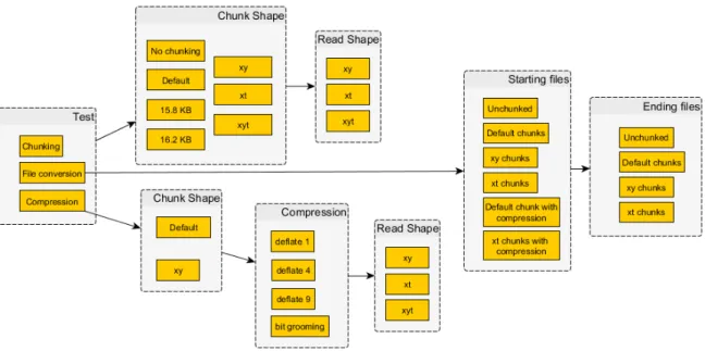
4 NetCDF4 Chunking and Compression Read Performance 50 4.1 Method . . . 52 4.1.1 Chunking performance . . . 53 4.1.2 Compression performance . . . 55 4.1.3 File conversions . . . 57 4.2 Chunking performance . . . 57 4.2.1 Results . . . 57 4.2.2 Discussion . . . 60 4.3 Compression performance . . . 61 4.3.1 Results . . . 61 4.3.2 Discussion . . . 64 4.4 Layout conversion . . . 64 4.4.1 Results . . . 65 4.4.2 Discussion . . . 65 4.5 Conclusions . . . 66

5 Parallel Reads from a NetCDF4 File to Improve Read Performance 69 5.1 Method . . . 71

(7)

Contents Contents

5.1.2 Parallel scaling . . . 73

5.1.2.1 Measurements . . . 74

5.1.3 MPI collective Method . . . 74

5.2 Parallel read scaling on JASMIN . . . 75

5.2.1 Results . . . 75

5.2.2 Discussion . . . 79

5.3 Collective I/O with MPI-IO and NetCDF4 . . . 82

5.3.1 Results . . . 82

5.3.2 Discussion . . . 82

6 Application to Atmospheric Science Workflow - Space-Time Spectral Analysis 88 6.1 Space-Time Spectral Analysis . . . 89

6.1.1 Relevance of STSA . . . 90

6.1.2 Example of STSA use . . . 91

6.1.3 Suitability as a case study . . . 91

6.2 Quantitative workflow analysis . . . 92

6.3 Method . . . 93

6.4 Results . . . 94

6.5 Discussion . . . 97

7 Conclusions and Further Work 102 7.1 Summary and conclusions . . . 102

7.2 Related work . . . 108

7.3 Further work . . . 112

Bibliography 114 A Platforms 122 A.1 JASMIN (Panasas) . . . 122

A.2 ARCHER (Lustre) . . . 124

(8)

Contents Contents B Tools 126 B.1 NetCDF4 C library . . . 126 B.2 MPI . . . 126 B.3 MPI-IO . . . 126 B.4 Nccopy . . . 126 B.5 Python libraries . . . 127 B.5.1 NumPy . . . 127 B.5.2 netCDF4-python . . . 127 B.5.3 H5py . . . 127 B.5.4 H5netcdf . . . 127 B.5.5 Jug . . . 128 C Code 129 C.1 Chapter 3, 4, and 5 . . . 129

C.1.1 Program to read using C from ’plain’ binary files . . . 129

C.1.2 Program to read using C from NetCDF4 files . . . 131

C.1.3 Program to read using Python from ’plain’ binary files . . . 134

C.1.4 Program to read using Python from NetCDF4 files . . . 135

C.2 Chapter 6 . . . 136

C.2.1 Read only test program . . . 136

(9)

Chapter 1

Introduction

The volume of data is growing in atmospheric science, as climate models increase to higher resolutions to improve the representation of atmospheric phenomena, and larger numbers of ensemble members are used so as to better capture the variability in the atmosphere. New methods need to be developed to handle the increasing size of data – traditional analysis scripts often inefficiently read and process data, leading to excessive analysis times. In order to make decisions on how to handle the large data sizes during application development and data management, quantitative analysis of the factors which affect data analysis throughput in atmospheric science in a high-performance computing environment are needed.

In general, there are four major stages to a workflow when analysing data in atmospheric science:

• First is accessing data. For smaller or medium sized datasets, it is often possible to down-load data to a local machine.

• Second is data exploration, important to assess suitability of a dataset for the investiga-tion, and to plan the investigation. Usually this is only on a subset of the data in which, even with large datasets, the volume of the data often is not problematic.

• Third is the development of the analysis application. This involves testing, which is often on a subset of the dataset, and will involve many iterations in development, meaning a large number of reads. This stage could also be skipped if existing applications exist from previous investigations.

(10)

Chapter 1. Introduction

tiple ensemble members, multiple time periods, or even multiple datasets (e.g. climate simulation output, and reanalysis data).

With very large datasets, transferring data to the user is not always an efficient option. In-stead, running applications local to a data storage and processing facility is a more efficient solution. One such example of this is the JASMIN (Joint Analysis System Meeting Infrastruc-ture Needs) super-data cluster.

Data exploration is inherently less data intensive than the final application, due to analysing only a subset of the data. However, any increase in duration due to inefficient reads or writes, is compounded with larger data sets.

Similarly to data exploration, because application development only requires a subset of data, it is not affected by inefficient reads and writes to the same extent as the final appli-cation. However, development and testing requires many repeated calculations, and read and write operations, meaning that any reduction in performance is compounded by larger datasets. With regards to the potential for existing applications being used, the processing al-gorithms may not be suitable for use with very large data, or could be significantly improved to provide acceptable run times. Bespoke applications or libraries, designed to analyse very large datasets are a good alternative to writing applications. However, analysis can often be too specific, or specialised for this approach to be valid, therefore, an application needs to be developed. Without prior quantitative knowledge on the factors which can affect analysis ap-plications, providing acceptable performance can become a very time consuming task, and development can become constrained by trial and error. This can significantly lengthen the development process, taking up time which could otherwise be used for further analysis, or results interpretation.

Research into large data analysis generally focuses on providing a solution in the form of a library, software middleware, or hardware to improve performance. The motivation for these studies is that data analysis on large data is a problem and will become more of a problem, generally with little quantitative evidence. For those with experience handling and analysing large data, the problem is obvious, as are the implications for analysis as we progress into the exascale. The aforementioned prior quantitative knowledge on the factors which affect analysis is a gap in the research, and the focus of the work presented in this thesis. This knowledge is often gathered through experience, and trial and error, so the usefulness for this study is clear – circumventing pitfalls due to combinations of effects which provide very poor

(11)

performance, and eliminating a large proportion of trial and error, will reduce development time and enable more science to be done.

In atmospheric science, little work has gone into understanding, quantitatively, how the software-hardware stack can affect analysis workflows. Weather and climate models are com-plex and much work has gone into what can affect their performance (Section 2.1) – the per-formance of analysis applications could be investigated in a similar way.

Reading and writing data is a major bottleneck for analysing data in atmospheric science (M´endez et al., 2013; Gao et al., 2011). This problem is only going to become compounded as data gets larger, due to increasing temporal and spatial resolutions needed to more accurately represent the physics and dynamics in models; and increased ensemble sizes, needed to more accurately capture uncertainty in the chaotic systems (Balaji, 2015).

Traditionally, analysis of atmospheric science data has been done in serial, although that is now changing. Serial data analysis on very large datasets can be problematic for a number of reasons. Firstly, large datasets mean that the random access memory (RAM) may not be large enough to hold the data during calculations. Secondly, analysis can take a long time to complete, slowing down the workflows and meaning some tasks can become impractical. Many different factors can affect how long an analysis program takes to run, such as:

• the time to read or write data, which is heavily affected by the data size,

• the analysis algorithm,

• the organisation of the data,

• and the hardware and software used.

Running analysis in parallel can alleviate problems with long run times and running out of RAM. When using multiple nodes in parallel, the RAM from each node can be used, increasing the amount of RAM proportional to the number of nodes. The I/O and compute can also be split amongst the nodes, decreasing the total time for the parallel program to run. There are complications to consider when designing parallel programs, any of which can contribute to an efficient or inefficient program. These include:

(12)

• the load balance for the I/O, computations, and RAM,

• the platform architecture and settings,

• and the inter-processor communication needed for the algorithm.

These factors can make writing an efficient parallel program difficult for many analysis tasks. Large datasets in atmospheric science are often stored in an archive, or filesystem of a data centre. This data is generally produced by some form of model or simulation, so is written once and read from many times, by many different users. Typically, reading data dominates other factors for performance of applications (Childs et al., 2005). Factors which can specifically affect the read rate for an algorithm include:

• the layout and format of the data (including multidimensional tiling, and compression),

• the read pattern of the algorithm,

• and the language and libraries used.

The combination of these factors produces a large, complex, and interdependent problem. Although these factors are interdependent, it is necessary to understand the individual effects on performance before their combination can be understood. This thesis investigates the con-tributing factors which can affect the read rate for serial and parallel atmospheric science data analysis scripts. The work approaches the effects on the read rate from the point of view of a user of a high performance computing (HPC) platform, rather than analysing the peak per-formance of a system. The peak perper-formance is not always useful to know when designing analysis programs, because the system performance is often quoted as a system wide perfor-mance, and the peak theoretical performance of a platform is often not representative of a real workflow. For example the theoretical I/O bandwidth may not be achievable. For climate and weather models, Balaji et al. (2017) discussed that, for example, flops (floating point opera-tions per second) is not a useful metric for examining performance of earth-system models, instead they proposed more relevant domain specific metrics, such as simulated years per day. In a similar way, identification and quantification of realistic factors affecting data analysis in atmospheric science would be more relevant to users than system level benchmarks.

There are three investigations in this thesis: 1) the effect of the read pattern, software, and data type on the read rate, 2) the effect the layout of the data has on the read rate, and 3) the

(13)

Chapter 1. Introduction 1.1. Thesis structure

scaling of the parallel read rate for multiple different situations. The final part of the investi-gation in this thesis is to implement the results from the first three investiinvesti-gations into a case study; affirming whether the results are valid in more realistic situations, and so applicable to the general users of HPC platforms. The JASMIN super-data cluster (Lawrence et al., 2012) is used throughout the thesis, as an exemplar HPC platform for data analysis (other platforms are used in sections of the thesis to provide a broader sample base).

1.1 Thesis structure

Chapter 2 contains the background required for the rest of the thesis, including: parallel com-puting concepts, factors affecting I/O performance, and discussion of parallel filesystems. The relation of these factors to atmospheric science is discussed, as well as alternative approaches to big data analysis. Chapter 3 contains the investigation of the performance of NetCDF4-python and the underlying libraries that it uses, as well as the effect read sizes and read patterns have on the read rate. Chapter 4 investigates how multidimensional tiling and compression affect the read rate. Chapter 5 investigates parallel scaling when reading NetCDF4 files on a parallel file systems. Chapter 6 combines work from the previous chapters in a case study, to ascertain whether the optimal parameters discovered the previous chapters are applicable to a real-life work flow. Then conclusions are drawn in Chapter 7, with discussion on how the thesis re-lates to other studies, and a discussion of channels for future work is included. Appendix A provides a more detailed look at the platforms used in the thesis than that in the background chapter. Appendix B describes the tools and libraries used for the testing scripts. Finally, Ap-pendix C contains the main code for the testing scripts used.

1.2 A note on file sizes and read rates

Throughout this thesis, both base 10 (e.g. MB) and base 2 (e.g. MiB) units are used. Table 1.1 shows the size of each unit in bytes and the size difference. Where both are used care has gone into making sure the units are reported correctly. Rates in this thesis are always reported in base 10 units. Base 2 units are used for reporting file sizes where the files created for testing were in in base 2. So that the reported file sizes are easier to read on both graphs and in the text, the base 2 units are retained, as opposed to converting to base 10 and reporting the file

(14)

Chapter 1. Introduction 1.2. A note on file sizes and read rates

as opposed to rounded for the sake of reporting in base 10).

Table 1.1: The sizes in bytes of base 10 and base 2 units.

Base 10 Base 2 Difference (B)

1 KB = 103B 1 KiB = 1024 B 24 1 MB = 106B 1 MiB = 10242B 48,576 1 GB = 109_B _{1 GiB = 1024}3_B _73,741,824 1 TB = 1012B 1 TiB = 10244B 99,511,627,776

(15)

Chapter 2

Background

In this chapter, overarching concepts important to this thesis are discussed, along with alter-native approaches to big data analysis.

A useful way of analysing the performance of a system is to categorise similar algorithmic patterns to predict performance (Section 2.2). I/O is a major bottleneck in atmospheric science so it is important to understand how to measure I/O performance (Section 2.3), as well as why data size is a problem in atmospheric science (Section 2.4). One way to improve performance of analysis applications in atmospheric science is to run them in parallel. This means that par-allelism needs to be understood (Section 2.5), along with what factors affect I/O performance (Section 2.6). In order to understand the results from investigating application performance, the platforms which analysis is performed on need to be understood (Section 2.7). There are many other valid approaches to dealing with atmospheric big data, some of which are outlined in Section 2.8.

2.1 Atmospheric science model performance

Having useful measurements of performance is an important aspect of understanding perfor-mance. The performance of climate and weather models is an important area of research, due to not only the computationally intensive nature of the simulations – due to increasing res-olution, complexity, and increasing ensemble sizes – but also the importance of the research providing scientific input to global policy decisions; for example the IPCC AR5 report (Stocker, 2014).

(16)

Chapter 2. Background 2.2. Categorisation as a method to analyse performance

credibly useful. Balaji et al. (2017) propose a set of metrics that are representative of the actual performance of the models. For example, flops are not always a useful metric, whereas the number of simulated years per day is a much more relevant. Developing a similar set of per-formance metrics for data analysis would allow better profiling of data analysis applications. The first stage of this is to identify the areas where performance is affected.

2.2 Categorisation as a method to analyse performance

Characterisation of patterns in data can be used to gain an understanding of a system. Like-wise, characterisation of different patterns in data analysis can help understand those applica-tions. Similar algorithms can then be grouped by their characteristics, and then analysed for the best way to implement the applications for use with big data. Future applications which fit into the same groups could be solved in a similar way, making it easier to efficiently write those programs.

The Berkeley Dwarves provide a way of looking at parallel HPC applications on multicore processors (Asanovic et al., 2006). With a similar aim, but with a focus on data analysis, the Big Data Ogres were proposed (Jha et al., 2014). The Ogres provide four key facets to aid the understanding of big data analysis. These are:

1. the problem architecture facet,

2. the execution features facet,

3. the data source and style facet,

4. and the processing facet.

The problem architecture describes the way in which the problem has to be solved, for instance in a pleasingly (or ebarrassingly) parallel way, using shared memory, or machine learning (these will be discussed in Section 2.5.4). The execution features describe limiting factors, such as the I/O balance with the compute, and the limitations imposed by big data (discussed in Section 2.6). The data source and style facet describes the data itself, such as whether it is binary file format or a database, or the source of the data. The final facet, processing, describes the specifics of the algorithm, such as search and query, graph algorithms, and local and global machine learning.

(17)

Chapter 2. Background 2.3. Measuring I/O performance

The Ogre’s facets can be more specifically applied to work in atmospheric science. Exam-ples of how each facet could describe problems in atmospheric science:

1. Problem architecture, for example, could be a pleasingly parallel problem involved with retrieval over images, or could be a machine learning algorithm clustering atmospheric phenomena.

2. The execution features depend heavily on the algorithm, especially the balance between I/O and computation time (I/O-CPU balance), the data size, and the number of different fields required for the analysis.

3. The data source and style would typically be binary data for climate analysis or weather forecasting, but could be other data types, such as CSV files, images, or a proprietary data type.

4. The processing algorithm describes the specifics of the algorithm, for example, the spe-cific clustering, or tracking algorithm.

In order for categorisation to be useful, an understanding and quantification is required for the factors which affect the performance. With analysis of large data sets in atmospheric science, typically I/O is a major bottleneck (Balaji, 2015).

2.3 Measuring I/O performance

Note that, throughout this thesis only reads will be discussed because data analysis on large data sets in atmospheric science is generally executed on data stored in an archive, which was produced by a numerical model. This means that reads are significantly more dominant than writes in most cases. Read performance can be quantified in different ways. Those discussed here are:

• read rate,

• bandwidth,

• I/O operations per second (IOPS),

(18)

The read rate measures the speed of the operation and is defined as the amount of data transferred per second, for example if 600 MB were transferred in one minute the read rate would be 10 MB/s. The bandwidth is the maximum potential performance limited by the hardware being used. The minimum bandwidth in a system will constrain the total bandwidth available, for example if a filesystem has a bandwidth of 10 GB/s, but the local area network has a bandwidth of 1 GB/s, the network would limit the maximum rate. Note that this is a theoretical limit imposed by the hardware, which may not be achievable in reality. IOPS (I/O operations per second) describes the rate of which I/O operations can occur, including both reads and writes. This is also a theoretical limit, and hardware often quotes maximums for reads and writes, for sequential (where the next I/O operation is the neighbouring piece of data) and random (where the next I/O operation is not the neighbouring piece of data) – the random IOPS is lower than the sequential IOPS. Finally, the throughput is defined as the IOPS multiplied by the size of the I/O operation, meaning to improve performance either the read size, or the IOPS needs to increase.

Benchmarking applications can be used to assess the I/O performance of a system, and this can be used to help understand how an analysis application would perform. Four different applications will be discussed here, however, none of these quantitatively assess where in the software-hardware stack performance is being affected, only the overall results – this provides motivation for the work in this thesis.

On Linux based systems, a simple way to profile I/O is using theddutility1. ddmeasures the read and write times and uses arguments to vary parameters, outputting the wall time (real-world time from start to finish for the application) and the respective read or write rate. It allows the size of the buffer to be varied. This controls the size of the individual reads and writes, for example a 1 GB read could have a buffer size of 1 MB, meaning 1000 reads were executed. The advantage and disadvantage ofddis its simplicity, as it only enables one-dimensional read and writes of binary data, and has no inbuilt way to assess parallel reads.

IOR2 is a parallel benchmarking application, which allows much more control than dd, giving options including: the file type (including NetCDF, and HDF – see Section 2.4), the number of parallel tasks, the buffer size, and the number of files per task. This allows the performance on parallel file systems, and HPC clusters to be assessed, and so predict how

1_{https://linux.die.net/man/1/dd}

(19)

parallel applications would perform. This is still a relatively simple benchmark however, and so may not be truly representative of the performance for scientific applications. An example of IOR results from JASMIN are shown in Figure 2.1.

IOR can be used to synthetically and accurately model applications (Shan et al., 2008). The-oretically, the arguments of IOR can be used to replicate the I/O of an application to measure how it would perform on a system without having to run the application, saving time. How-ever, the opinion of some studies is that it can be difficult to relate the IOR arguments to real applications (Borrill et al., 2007; Lawrence, 2014).

Figure 2.1: I/O scaling results from JASMIN using IOR measuring total bandwidth (y-axis, in GB/s) scaling with number of shelves (See Appendix A). Figure from Lawrence (2014)

Benchio3 was designed to give a more flexible benchmark which is more applicable to scientific analysis than IOR (Lawrence et al., 2017). Firstly, it provides more control of the parallel decomposition to more accurately represent read patterns in applications. Secondly, it is less opaque than IOR, enabling more conclusions to be drawn about what is affecting the I/O rate. Finally, benchio is able to use three-dimensional data, meaning it is much more relevant for scientific applications.

MADbench2 (Borrill et al., 2009) is an application derived benchmark, developed from analysis of the cosmic microwave background (electromagnetic radiation which can provide information on the early universe). It provides more information than the previous bench-marks discussed above, including the time spent in CPU based calculations, and the I/O time. It allows adjustment of the scale of the benchmark, parallelisation, and system specific settings. The aim of this benchmark was to measure and compare the performance of systems rather than predict quantitatively how other applications would perform.

(20)

Chapter 2. Background 2.4. Atmospheric science data

Instead of measuring the performance of applications directly, statistical modelling can be used to predict the performance of the applications by identifying important elements of the access path. Schmid and Kunkel (2016) showed that artificial neural networks can more accu-rately predict performance than a linear model, where linear models are not a valid method of performance analysis.

2.4 Atmospheric science data

For a given analysis problem, the data size affects the number of floating point and I/O op-erations, each of which can increase the run time. Higher fidelity models and observations, and larger ensemble sizes produce larger amounts of data, all of which needs to be analysed. For example CMIP6 is expected to produce 10-20PB of data (Cinquini et al., 2014), compared to CMIP5 which produced around 3 PB (Liu et al., 2015). As the data size becomes larger, the analysis problem becomes more difficult.

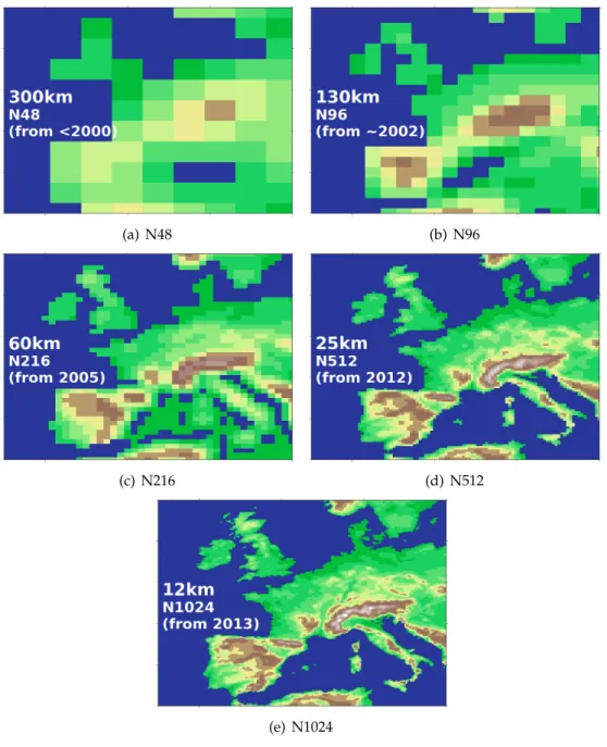
Higher spatial resolutions provide a number of benefits for atmospheric models. Firstly, high horizontal and vertical resolutions mean that atmospheric phenomena and topography are more accurately represented (demonstrated in Figure 2.2), improving the accuracy of mod-els. Secondly, with higher resolutions less parametrisation (representing phenomena with pa-rameters when they are not resolvable) is needed, potentially improving the accuracy of mod-els. For instance, at higher resolutions (around 1km) convection is resolvable.

Higher temporal resolutions are often required to ensure stability with higher resolution models. Also, higher temporal resolutions can resolve phenomena more accurately. Quite often, not all timesteps are outputted from the model – either timesteps are skipped when saving the data, or an average is calculated over a time period, and the result saved. Higher temporal resolutions are needed when analysing models if fast moving phenomena are being studied, such as gravity waves.

Ensembles are used to capture variability in chaotic systems. Each ensemble member has slightly different initial conditions, so each will have a different representation of the atmo-sphere. The variability in the atmosphere is more accurately represented by having a larger number of ensemble members, but this also means there is more data to analyse.

The volume of data in atmospheric science is a problem since I/O is a major bottleneck (M´endez et al., 2013; Gao et al., 2011). With traditional, serial analysis programs which are

(21)

often either made for a very specific task, or are legacy programs which were used for analysis on smaller data sets, the program may not complete the analysis in a timely manner. The latter is an obvious problem, but the former is a problem from a productivity standpoint – having to wait a long time for analysis to finish degrades productivity. Analysis programs taking less time, and producing results faster also means that more science can be done.

Before discussing an example of why big data is a problem in atmospheric science, the nomenclature of the resolution of atmospheric models needs to be described. Figure 2.2 shows an example of the nomenclature used with climate models to describe the resolution (this nomenclature is used for the MetOffice Unified Model, other models may use different nomen-clature). Nxdescribes the horizontal resolution according to the formula[2x,3x/2], for instance N216 has 532 longitude points, and 324 latitude points, N512 has 1024 longitude points and 768 latitude points, and N2048 has 4096 longitude points and 3072 latitude points – the number of points for all the resolutions in Figure 2.2 is shown in Table 2.1 (plus N2048). The number of levels in the model is then describe by an L followed by a number, i.e. L80 has 80 vertical levels, and L180 has 180 vertical levels. This is combined to give a spatial description of the model, e.g. N512L180 would have dimensions (in height, latitude, longitude order) of [180,768,1024] – this order is used in the thesis to describe the slowest to fastest varying dimension.4

Table 2.1: Number of latitude and longitude grid points for each resolution. Resolution Longitude Latitude Size in MB

N48 96 72 0.055 N96 192 148 0.22 N216 512 324 1.33 N512 1024 768 6.3 N1024 2048 1536 25 N2048 4096 3072 100

As an example of why data volume is a problem for atmospheric analysis, consider the following when analysing stored data (most analysis in atmospheric science is done post run-time, when the data is stored in an archive, or analysis platform). In the first case consider results from an atmospheric simulation run for 1 year with a 6 hourly timestep and a middling resolution of N216L80, meaning the dimensions are [1440x80x324x512]. This means the dataset has a size 152 GB with each element an 8 byte floating point numbers. At peak read rate of 1GB/s (the approximate theoretical maximum for a serial process on JASMIN (Lawrence et al., 4_{Longitude values for the first latitude value and height value are contiguous on disk, followed by the next set}

(22)

(a) N48 (b) N96

(c) N216 (d) N512

(e) N1024

Figure 2.2: Representation of Europe in the different resolution models as part of a global model. Blue denotes sea, and the other colours denote the elevation of land.

2012)), this read would take around 152 seconds. At a realistic inefficient read rate of ap-proximately 10MB/s (from the investigation into read performance in Chapter 3), this would increase to 253 minutes – a significant increase but not unreasonable.

Now consider the same analysis on high resolution N512L180 hourly data, with dimen-sions of [8640x180x768x1024] – 9.8TB in size. At the 1GB/s read rate it would take 163 minutes to read the data, however at 10MB/s it would take 11.3 days to read the data - obviously impractical. At even higher resolution this problem would be compounded. As well as resolu-tion, when analysing ensembles this must be multiplied by the number of ensemble members. There are a number of ways to potentially improve the read rate: identifying where there

(23)

are factors influencing the read rate (Section 2.6), implementing the analysis in parallel (Section 2.7), along with other techniques discussed in Section 2.8.

One of the most widely used data formats in atmospheric science is the Network Common Data Format (NetCDF)5_{. Figure 2.3 shows an example of the proportion of data stored in the}

JASMIN workspaces. NetCDF4 is built on HDF5 (Hierarchical Data Format version 5). (Note, NetCDF3 is an older format of NetCDF not built on HDF5, and does not allow chunking (see Section 2.4.1) so is not investigated in this thesis, for a comparison between NetCDF3 and 4 performance see Welch et al. (2010)).

1-9B 10-99B

_100-999B

1-9kB

_10-99kB

100-999kB

1-9MB

10-99MB

100-999MB

1-9GB

10-99GB

100-999GB1-10TB

0 1,000

2,000

3,000

4,000

5,000

6,000

Volume (TB): All

bundle

code

figs

hdf

nc

other

pp

txt

wmo

Figure 2.3: Data stored at JASMIN on the group work spaces (June 2017), split into the file size(x-axis), total volume (y-axis), and the composition from different file types. (B.Lawrence, personal communication) Note, the histograms are stacked.

2.4.1 HDF5

HDF5 is a versatile, portable data format which can be used to store large data sets, and it allows the use of chunking and compression6_{. Chunking (an implementation of}

multidimen-sional tiling) allows files to be reorganised on disk to improve read rates for different access patterns (Welch et al., 2010) – discussed in Section 2.6.3. Chunking can improve the perfor-mance of partial I/O (when only sections of the file are being read) (Rew, 2013). This is

(24)

be-Chapter 2. Background 2.5. Parallelisation

cause, in order for partial I/O to be most efficient the data selected must be contiguous on disk, which chunking allows. The chunks can be compressed to reduce the size of data on disk – compression is discussed in Section 2.6.4. Chunking and compression can have a large effect on the read rate (Bartz et al., 2015).

2.4.2 NetCDF4

NetCDF4 is popular in the scientific community because it is a self describing, platform in-dependent binary file format. NetCDF4 allows the use of zlib compression (Lee et al., 2008) which allows sections of the file to be compressed and accessed individually (in this case the sections are chunks) – compression is discussed in more detail in Section 2.6.4. zlib compres-sion provides a good balance between comprescompres-sion ratio and comprescompres-sion speed (Liu et al., 2015) without losing accuracy in the data (lossless compression). The data size is reduced so less data is read from disk, meaning the time to read the file could decrease (Miller, 2015), but obviously this data will then need to be uncompressed on the processing node, meaning there is a balance between increased read rate due to fewer bytes being read, and the extra compu-tation required to uncompress the data. The compression of NetCDF4 requires the data to be chunked so the interplay between chunking and compression could have a significant effect on the read rate. The author is not aware of any literature which looks at how the interplay between compression and chunking affects the read rate.

2.5 Parallelisation

Running an algorithm in parallel means splitting an algorithm into sections and running these sections on multiple processors. If these section are run simultaneously they are concurrent. This may be done because of the volume of work (calculations or I/O) in the algorithm, or because a single node does not having enough memory to process the data required (utilising multiple nodes can increase the effective memory available for the algorithm). Parallelising an algorithm into multiple tasks can reduce the time for an algorithm to complete. Parallelisation on multiple nodes also means utilising more network interface cards (NICs), increasing the available I/O bandwidth; so that if the I/O is run in parallel, the I/O time can be reduced. This last point is important as it is well known that I/O is a major bottleneck for analysis in atmospheric science, serial data processing is no longer an optimum solution (Balaji, 2015),

(25)

Chapter 2. Background 2.5. Parallelisation

and concurrent reads are crucial for high speed reads (Lofstead et al., 2011).

2.5.1 Strong and weak parallel scaling

Strong and weak scaling is an important concept for analysing results with parallel application performance. Strong scaling is where the size of the problem stays fixed, but the number of concurrent tasks is increased. Weak scaling is keeping the size of the problem per task the same, but the total size of the problem increases with the number of tasks. An example of the difference can be demonstrated when reading data to test the I/O scalability of a system. In the strong scaling case a single task could read from a 1 GB file, then two tasks would either read half the file each, or two 500 MB files – keeping the total size the same. In the weak scaling case, with two tasks, each would read from a 1 GB file – the total size of the problem has doubled.

2.5.2 Amdahl’s Law and Gustafson’s Law

In its simplest sense, parallel computing is purely using more than one processor to complete a task. However, the proportion of a workflow which must be executed in series limits the available speedup (the parallel algorithm’s time to complete divided by serial algorithm’s time to complete). With a fixed problem size this is described by Amdahl’s law, which gives an upper, theoretical, limit on how much a task can be sped up, depending on how much must be executed in serial. The maximum speedup of a task is described by:

R(P)/R(1) = 1

S+ (1−S)/P (2.1)

whereR(P)is the rate of completion of a task usingP processors andS is the fraction of the time spent doing tasks in serial (Amdahl, 1967). In an idealised situation using an infinite number of processors, the maximum speedup is maximum1/S, so for example for a process in which 10% must be done in serial, the maximum speed up is 10 times.

Gustafson’s Law does not assume a fixed problem size (strong scaling), and instead as-sumes that as the computational power of a system increases, more work will be done (weak scaling) (Gustafson, 1988). This gives no limit to the possible speedup when the problem size increases.

(26)

2.5.3 Flynn’s Taxonomy

Flynn’s taxonomy is a classification scheme for central processing units (CPUs). There are four classifications, which are described by the number of instruction or data streams are being used, this is shown in Table 2.2. SISD (single instruction multiple data) is where a single pro-cessing unit (PU) receives a single instruction stream from memory and a single data stream, giving a single operation at a time; an example of this would be old single core personal com-puters (PCs). MISD (multiple instruction single data) describes when multiple instructions streams operate on the same data. MISD is generally used for fault tolerance, where all results from the instruction stream must agree. SIMD (single instruction multiple data) describes a computer in which a single instruction stream works on different streams of data working in parallel to process data faster with no parallelisation of the instruction stream. An example of SIMD would be a graphics processing unit (GPU). MIMD (multiple instruction multiple data) on the other hand, parallelises the instruction stream and the data stream, an example of which would be a modern PC or cluster. (Flynn, 1972)

Table 2.2: The four types of computer architecture according to Flynn’s taxonomy. Single instruction stream Multiple instruction streams

Single data stream SISD MISD

Multiple data streams SIMD MIMD

MIMD can be further divided into SPMD (single program multiple data), and MPMD (mul-tiple program mul(mul-tiple data). These two roughly describe different techniques to parallelise workflows: either as a single program executing on different sections of data, to process the data faster, which could also be described as data parallel or domain decomposition; or multi-ple different programs where sections of the workflow are split between processors, this could also be called task parallel (Blank and Nickolls, 1992). Typically, data parallelisation is the dom-inant form of parallelisation on modern computers (MIMD type) (Hager and Wellein, 2010). Typically, most applications, however, will use a combination of data and task parallelism.

2.5.4 Parallel computing models

During the discussion on Big Data Ogres in Fox et al. (2014)(the key facets were discussed in Section 2.2), there were five computing models described (the problem architecture facet). It is important to discuss the relevance of these computing models for the work in this thesis. These are:

(27)

• classic MapReduce,

• iterative Map-Collective,

• iterative Map-communicative,

• pleasingly (or embarrassingly) parallel,

• and shared memory .

The MapReduce and pleasingly parallel models are shown in Figure 2.4. All of these in terms of Flynn’s taxonomy would, for most workflows, be classed as SPMD, or data parallel.

Figure 2.4: Representation of the three families of MapReduce, plus pleasingly parallel (or map only). From Fox et al. (2014) (Figure 2).

The first family of MapReduce is commonly known as classic MapReduce; it was the orig-inal version of MapReduce introduced by Google (Dean and Ghemawat, 2008). In this version of MapReduce the input data or input files are split and sent to map functions which then perform some algorithm, which, for example, could be a sort or search algorithm. The results from the map stage are then sent to the reduce stage where a function typically will summa-rize the results from the map stage, or could merge values to give a smaller set of results. Typically MapReduce is used for analysis tasks such as web based big data, but there has been some work on how to extend this to scientific data (see Section 2.8 for a discussion on some approaches).

The other two families of map reduce are iterative Collective and iterative Map-Communication. The former uses a collective stage to gather data and recast it out for another iteration of the algorithm. A common implementation of this would be in clustering, where data is collected into regions over a number of iterations, becoming more accurate after more iterations of the algorithm. Map-Communication has the communication included as part of

(28)

Chapter 2. Background 2.6. Factors affecting I/O performance

the processing algorithm (before the reduce) and is also iterative. An example of the use of this would be for solving graph algorithms.

Pleasingly (or embarrassingly) parallelism is in many ways similar to MapReduce, but with no reduce stage. Like the map stage of MapReduce, the input data is split between processors and these processors implement an algorithm. There is no communication between processors. Shared memory is a technique that allows multiple processors to access a large pool of memory, negating the need for explicit communication between the processors, because they can all access data in the memory.

2.6 Factors affecting I/O performance

Many factors can affect the read performance of analysis. Figure 2.5 depicts factors which can affect the read performance, and from what area of the software-hardware stack they originate. The I/O time is affected by the size of the data, the software, the bandwidth defined by the hardware, and the access pattern to the data. The size of the data and the system settings are generally not adjustable by the user implementing the analysis – the system options, such as stripe width, are sometimes configurable but often users do not configure them. It is well known that access patterns and data organisation have a large impact on I/O rate and can dominate other costs in analysis (Childs et al., 2005). How the software and hardware, and the tunable parameters chosen either by the user or the system administration, interact can also have a large impact on the I/O rate and therefore affect the workflow.

Figure 2.5: Factors which can affect the read rate for a program. The blue boxes show in which section of the software-hardware stack each factor is contained.

(29)

can have a significant effect on the read rate. Before going into detail about access patterns, it is useful to discuss how data is accessed on a hard disk drive (HDD).

2.6.1 Data access from a HDD

Data is stored on disk as a one-dimensional stream of bytes. The relation between the logical order in array space and file space is depicted in Figure 2.6. When the file system requests data from a storage disk, the read head is moved to the correct distance from the centre of the disk so that the correct track on the disk is selected – the track is the path covered by the read head as the disk rotates. The time for this movement of the read head to the track is called the seek time. Once the head is on the correct track, it needs to wait for the data to move under the head, this time is known as rotational latency. The total time to access the data on the disk is the sum of these two times. The initial part of data read from the sector is the header (a sector being the smallest amount of data that can be read or written to disk) and the last part of the sector is the trailer. A header defines the start of the sector and contains metadata about the sector. The trailer defines the end of the sector and contains error correcting code for the sector. This is not to be confused with the header for a file, which can contain metadata on the file. A file is composed of many sectors. The mapping between files and sectors is controlled by the file system. A file is composed of many of these sectors, which, in an idealised situation or clean disk, are stored in order (in practice files will be fragmented, or spread, throughout the disk). (Silberschatz et al., 2013)

Figure 2.6: Relationship between the logical layout of the data in array space (left), and file space (right). The fastest varying dimension is labelled ’Dim 1’.

Data is stored as a one-dimensional stream of bytes, so understanding how this translates to multidimensional data is important. In the array order, the fastest varying dimension (x in the examples here) sits contiguous on disk for the first value of y, z, and t. The next set of x values, for the second y value and first z and t, lies next on disk. Once y has reached its

(30)

in Figure 2.7(a) (in this example there are 4 x, 2 y, 2 z, and 2 t values).

2.6.2 Read patterns with multidimensional arrays

The read pattern can have a significant effect on the read rate. Figure 2.7, and 2.8 shows an example of how the read pattern affects the read rate. With the ’normal’ laid out file, the x-t read would be a non-sequential read, which severely reduces the read rate. One technique to avoid this would be to rearrange the data in the file, either by changing the layout of the files (Dong et al., 2013), or by using multidimensional tiling (Section 2.6.3). By optimising the read rate for one read pattern, the read rate for other read patterns can be handicapped. One strategy to avoid this is to store multiple versions of the data. This is not an ideal solution, however, because it increases data storage costs, although compression can reduce this cost by reducing the data volume. Compression of data could also increase the read rate because of less data being read from disk (Baker et al., 2014).

(a)

(b)

Figure 2.7: Demonstration of the effect of multidimensional tiling to the logical layout of a file in 1D. The blue colour shows an x-y read and red shows an x-t read. (a) shows the normal layout of the file with no chunking applied – x varying first, then y, z, finally t until the end of the array. (b) shows a layout with a chunk shape that contains all x and t – x varies, then t, then y, z until the end of the file. This means that a read in x-t space will read significantly faster in (b) than (a), but the x-y read will be slower.

2.6.3 Multidimensional tiling

Multidimensional tiling is where the logical order of the array is maintained, but the order of bytes on disk is changed, depicted in Figure 2.9. An example of this would be in Figure 2.7

(31)

Figure 2.8: Same as Figure 2.6, but with the red box showing how a slice in array space relates to the access pattern in file space.

– when the tiling has changed the order of the file to [z,y,t,x], the arrays are still indexed as [t,z,y,x]. This is a trivial example, but keeping the logical array indexing the same is important in cases where the chunking does not just change the order of the dimensions. For instance, the tiles could be small hypercubes a tenth of the size of each dimension; if this changed the way to index the array it would significantly complicate analysis scripts. The flexibility of multidimensional tiling allows the performance of many different read patterns to improve, but at the cost of the performance of others. An implementation of multidimensional tiling is HDF5’s chunking.

Figure 2.9: Same as Figure 2.6, but with multidimensional tiling applied to the file, giving four chunks. The layout is changed so the access pattern in the red box is contiguous in file space. The yellow boxes show where the file size has been increased because of the mismatch between the tile shapes and the array dimensions.

2.6.4 Compression

Compression reduces the size of data by using an algorithm to discover patterns in the data, so that the file can be represented as repetitions of patterns in the file; reducing the amount of bytes it takes to represent it. There are many different types of compression algorithm, which fall into two main groups, either lossy, or lossless compression. Lossless compression compresses the data without losing any accuracy in the data. Lossy compression however does reduce the accuracy of the data: it identifies unimportant information and removes it from the data (Huang et al., 2016).

(32)

imple-Chapter 2. Background 2.7. Parallel data analysis in a HPC environment

edge of the data itself. The algorithm then identifies redundancy in the byte stream. This method is generally not very effective with floating point numbers. The second method in-troduces some prior knowledge about the data type, so is more effective with floating point numbers. However, the floating points are still treated as a one-dimensional array, so it does not perform well with scientific data, where redundancy is often in higher dimensions. The third method applies more prior knowledge about the data, including the relationships be-tween the dimensions. This allows redundancy to be identified along multiple dimensions, which allows greater levels of compression for scientific data. However, this method is slower. It is well known that floating points do not compress particularly well with lossless com-pression (H ¨ubbe et al., 2013). An example of a lossy comcom-pression method could reduce the accuracy of the data, removing non-scientific, essentially random, data by reducing the signif-icant digits of the data and so reducing the number of bits needed to store the data when con-verted to integers using a scale and offset (Zender, 2016) (reducing the accuracy of the floating point numbers is not suitable for every work flow, for example, budget studies). Bit grooming is an example of this method, and is similar to the more well known method, ’bit shaving’. Bit shaving converts the floats to integers by multiplication by the number of decimal places, then sets numbers beyond the number of significant digits (nsd) to 0 (Caron, 2014); introducing er-rors as an underestimation of the true values. Setting the bits to 1 instead overestimates the true values. Bit grooming alternates between 1s and 0s giving a better estimation of the true value (Zender, 2016). The data is still stored as floats in the NetCDF4 file, so not reducing the size of the file – it needs to be compressed in order to gain the benefit of reducing the number of significant digits. This method can improve the effectiveness of NetCDF4 compression.

2.7 Parallel data analysis in a HPC environment

A HPC data analysis cluster is composed of, generally, two components: a processing cluster, and a parallel file system. Each are connected via a high-speed network, and can consist of homogeneous (all the same), or heterogeneous (not all the same) nodes.

2.7.1 Compute cluster

Processing nodes in a HPC compute cluster are connected to each other via a network, and to a filesystem. Each node consists of one or more multicore processors with memory which

(33)

Chapter 2. Background 2.7. Parallel data analysis in a HPC environment

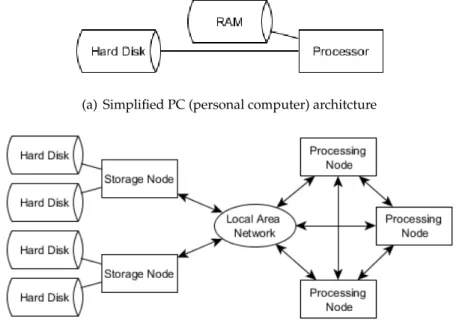
all cores can access. Comparing a personal computer (PC) and a HPC cluster (Figure 2.10), a PC consists of typically one multicore processor, and HDD (or other drive), which are directly mounted, whereas the connections to the storage system in a HPC cluster are over a network. Access to a HPC cluster is usually by a batch queuing system, allowing jobs to be submitted to be processed.

(a) Simplified PC (personal computer) architcture

(b) Simplistic schematic of a HPC cluster with parallel file system. The processing cluster is on the right composed of processing nodes, and the file system is on the left composed of storage nodes and hard disks. NB a processing node consists of RAM and a processor.

(c) Hadoop type cluster

Figure 2.10: Comparison between a typical PC, and a HPC cluster (a) and (b), and a parallel filesystem and distributed filesystem (b) and (c). Lines denote direct mounting, and arrows denote a network.

(34)

Chapter 2. Background 2.7. Parallel data analysis in a HPC environment

2.7.2 Parallel file systems

A parallel file system consists of multiple storage nodes connected to a network, designed to store large volumes of data, with fast (often parallel) access, while also providing a global shared namespace for directories and files. The shared global namespace allows access of the data without the user needing information about which specific nodes or disks the data is stored on – this is handled via metadata in the filesystem. A distributed filesystem (an example of which is Hadoop, shown in Figure 2.10) is also designed to store large volumes of data for fast access. The differences are that:

• On a distributed file system, each file is stored on a single node, whereas on a parallel file system a file can be split over multiple nodes.

• With a distributed file system, the storage is often, but not always, directly mounted to the processing nodes, whereas a parallel file system will be separate from the processing nodes.

To determine how a file is split between disks and nodes, a RAID (redundant arrays of in-dependent disks) algorithm is often used to ’stripe’ the data (see Figure 2.11) – note RAID algorithms are also used in non-parallel filesystems where multiple disks are used. Both RAID and parallel filesystems can be used to improve I/O performance.

Figure 2.11: Same as Figure 2.6, but with striping applied to the file. In this example, the file is split between two disks in a round-robin style, where alternate stripes are stored on each. (Note, this example shows RAID0 because no redundancy is included.)

A RAID algorithm can offer improved access speed or redundancy for data, depending on the type. The most important types of RAID algorithms to discuss here are RAID 0, RAID 1, and RAID 5. RAID 0 is where the files are ’striped’ across multiple disks to improve the trans-fer rate – striping is where the blocks (small elements of the file) are spread across multiple disks. RAID 0 does not provide any redundancy. RAID 1 is where the disks have a mirrored copy. This provides strong redundancy, and increased access speed, but is expensive for large

(35)

Chapter 2. Background 2.8. Alternative approaches to handling big data

volumes of data. RAID 5 uses the same striping idea as RAID 0, but with redundancy pro-vided by distributed parity. Parity is a system which can be used to detect errors in data and reconstruct it (Silberschatz et al., 2013).

The way the data is distributed in a parallel file system can have a large effect on I/O per-formance. The data distribution will depend upon the parallel file system settings, including RAID, stripe width (size of the stripes), and a minimum file size for striping. A logical file is a stream of bytes, in a parallel file system this is split amongst multiple nodes, and where each section of the file is stored is controlled by a manager node, transparently to the user. The dis-tribution is often a round-robin disdis-tribution as shown in Figure 2.11. Using multiple storage nodes enables greater maximum achievable bandwidth to the data, however, the performance could also be affected by the relationship between the read and the stripe width – performance is best when the read matches the stripe width – and likewise, multidimensional tiling will interact with the striping.

More specific details on the platforms used in the thesis are included in Appendix A.

2.8 Alternative approaches to handling big data

The aim of this thesis is not to compare different approaches to parallel data analysis, but to provide quantitative knowledge about factors which affect the I/O performance in a workflow; to provide more general information for developers of software and users of HPC clusters. However, there are many projects looking to improve parallel analysis. Some are outlined here.

Parallel libraries, particularly in Python, attempt to implement parallelism with minimal effort for the user. For example, DistArray7 _{aims to have a similar API to the Python library}

NumPy (popular array based data processing library), but to parallelise operations by using distributed arrays. Another library, Dask8, represents parallel computations as a task graph, with each operation represented as a node, and the vertices describing how the operations interact. A task scheduling algorithm then implements the graph in parallel.

Middleware (software which sits between the application and operating system), can be used to improve the I/O speed either by implementing the I/O in parallel (MPI-IO9),

continu-7_{http://docs.enthought.com/distarray/} 8_{https://dask.pydata.org/en/latest/}

(36)

Chapter 2. Background 2.8. Alternative approaches to handling big data

ously characterising I/O patterns to improve the parallel access (Darshan10), or separating the I/O from the application allowing the same script to be run on different platforms efficiently (ADIOS11).

ADIOS is middleware which allows an application to decouple from the platform I/O (Lof-stead et al., 2008). ADIOS provides a system to describe the data and platform specific factors outside the application through a simple configuration file, meaning that a single application can be effective on multiple platforms. ADIOS also has the ability to use BP (binary packed) files, which gives beneficial performance for reads along multiple dimensions (not normally the case, see Section 2.6) for data with greater than two dimensions with large files (Lofstead et al., 2011). This could solve many of the problems for large data analysis in atmospheric science, if a similar technique was applied to NetCDF4 files.

MapReduce and Hadoop are commonly used in BigData analysis in fields other than at-mospheric science. Their advantage is that they easily allow large scale parallelisation across clusters (Dean and Ghemawat, 2008). However, for scientific data, the MapReduce model may not work well because of the mismatch between the logical layout of the data in dimension space, and the physical layout on disk. Buck et al. (2011) aimed to provide metadata about the dimensionality of the data to the Hadoop framework in order to improve its performance with scientific data. Another approach to using Hadoop for processing scientific data is to provide HPC levels of performance to Hadoop-like workflows (Jha et al., 2014). Spark12is an adaptation of Hadoop which reduces I/O operations by keeping data in memory. SciSpark is an extension of Spark to scientific data (Palamuttam et al., 2015), which could give signifi-cant benefits to big data analysis in atmospheric science. H5Spark (Liu et al., 2016) is another similar approach of using Spark with atmospheric data.

Along with the more general tools and approaches above, another way of providing good performance for big data analysis is to create bespoke applications, or software suites. This allows any complicated programming to be implemented by software engineers, in order to free up scientists to focus on scientific analysis. An example of this is OODT (Mattmann et al., 2006). Some other technical solutions are described in Schnase et al. (2016) and Crichton et al. (2012).

In the concluding chapter of this thesis, the results from Chapters 3-6 are compared with 10_{http://www.mcs.anl.gov/research/projects/darshan/}

11_{https://www.olcf.ornl.gov/center-projects/adios/} 12_{https://spark.apache.org/}

(37)

Chapter 2. Background 2.9. Summary

other relevant approaches from literature, some of which are not discussed here.

2.9 Summary

There are many factors which can affect the performance of an application. The key bottleneck to analysis application performance for atmospheric big data is the read rate. Generally, the work which has been discussed in this chapter assesses how an application will perform on a specific system, or provide some ways of dealing with large data sets. What is not quanti-tatively investigated is how each layer of the software-hardware stack would affect an appli-cation. This is crucial in order to make application design decisions before development and assess how categories of analysis would perform. This thesis provides the first steps to this: when considering the analysis which needs executing, what factors affect performance, and so what design decisions should be made to avoid poor performance. Figure 2.12 shows which factors affecting read performance are being analysed in each chapter of the thesis.

Figure 2.12: Different factors that can affect read performance, with the different colours show-ing what chapter in the Thesis they are investigated in: green is Chapter 3, red is Chapter 4, and orange is Chapter 5. White boxes are not investigated.

(38)

Chapter 3

NetCDF4 Performance on HPC Parallel

File Systems

NetCDF4 (see Section 2.4.2) is frequently used in atmospheric science (See Figure 2.3), as is Python. The NetCDF4-python library is a very commonly used interface to NetCDF4 files with Python, and other libraries are often built using it. An important aspect of NetCDF4, which also makes it popular, is the ability to chunk and compress the data (see Section 2.4.2, and Chapter 4). The performance studies investigating NetCDF4 mainly focus on the performance compared to NetCDF3 (Lee et al., 2008), or as part of another library. An important first step in investigating the effect on read rate from the software stack, is to establish the baseline performance (meaning the best possible serial performance) when using netCDF4-python and NetCDF4 files. As far as the author is aware there are no published studies which investigate the performance of NetCDF4 in a serial implementation on HPC parallel file systems.

Analysing the performance of NetCDF4 for typical scientific workflows is critical, and is the first stage in determining the effect on the read rate of chunking, compression, and parallel reads.

The aims of this chapter are to:

• Evaluate the performance effect of using NetCDF4-python, and assess the reasons for any reduction in performance.

• Evaluate the effect on the read rate for different read patterns and read sizes.

Knowledge of any effect on performance from factors outlined in the aims will enable de-cisions to be made on what combination of factors gives the best compromise for read rate for

(39)

Chapter 3. NetCDF4 Performance 3.1. Methodology

large data sizes, and for different read patterns. Also, this knowledge will enable the identifica-tion of bottlenecks in the I/O pipeline and whether the effect can be mitigated, or the problem solved. The results from this chapter will provide a comparison for investigations into chunk-ing and compression (Chapter 4), parallel reads from NetCDF4 files (Chapter 5), and the effect on read rate for realistic workflows (Chapter 6).

Literature on the performance of NetCDF4 generally looks at the performance compared to previous versions of the library, with performance examples of new features (Lee et al., 2008). They do not assess the performance which would be seen from a typical user’s perspective. The reason for this is that each work flow is very different and there is not a general solution for every work flow and machine architecture.

The contributions from this chapter are:

• Quantitative read rate analysis from NetCDF4 files under a typical HPC analysis envi-ronment for atmospheric science.

• Comparison between the performance of the NetCDF4 C library and the netCDF4-python library.

• An evaluation of serial NetCDF4 performance on three UK atmospheric science HPC platforms: JASMIN, ARCHER, and the RDF, each of which has a different type of parallel file system (see Appendix A for details).

This chapter has been published in Jones et al. (2016), copies of which are available on request.

3.1 Methodology

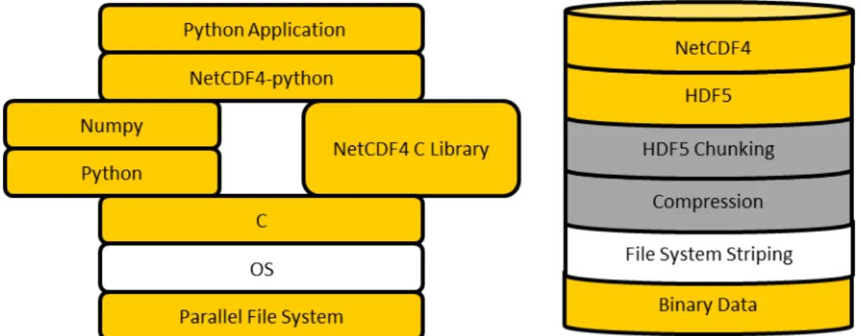
Performance is affected by different layers of the software stack shown in Figure 3.1. The yellow shaded boxes show the variables being investigated in this chapter, and the grey boxes show the variables tested in Chapter 4. The variables for each test are summed up in Figure 3.2. These variables are ones which a scientist wanting to do analysis can easily change, or are factors which could affect the performance further up the stack.

(40)

Chapter 3. NetCDF4 Performance 3.1. Methodology

Figure 3.1: The left image shows the software stack for applications built on NetCDF4-python. The netCDF4-python library relies on python (some of which is written in C) and the C NetCDF library. C interfaces with the operating system (OS) which interfaces with the par-allel file system to access the NetCDF4 data files. The right image depicts the NetCDF4 data format. NetCDF is built on HDF5, which is a type of binary file. Boxes shaded in yellow are being tested in this chapter, and areas shaded in grey will be covered later in the thesis.

Figure 3.2: Testing domain for this chapter, each box showing the variables, and each group showing the category they lie in.

3.1.1 Testing Domain

The main investigation in this chapter is into the effect using netCDF4-python has on the read rate. In addition, the file type and language were varied in order to identify any reduction in performance in the software stack, this being necessary to localise the cause of any impact on performance. Multiple file systems were used (by execution on different platforms) not as a comparison between platforms, but to provide a wider test base to strengthen conclusions. However, it is also a useful comparison to ascertain whether there is any difference in perfor-mance between the platforms.

There are factors which can be varied in the OS and parallel file system related to how the file system handles the data (storage location, and strip width for example), and how the OS