Data-driven Decision Support for perishable Goods
Inauguraldissertation
zur Erlangung des akademischen Grades eines Doktors der Naturwissenschaften
der Universität Mannheim
vorgelegt von
Jakob Huber
aus Ludwigshafen am Rhein
Korreferent: Prof. Dr. Nikolaos Kourentzes, Lancaster University, United Kingdom
Abstract
Retailers offering perishable consumer goods such as baked goods have to make hundreds of ordering decisions every day because they typically operate numerous stores and offer a wide range of products. Daily decisions or even intraday decisions are necessary as perishable goods deteriorate quickly and can usually only be sold on one day. Obviously, decision making concerning ordering quantities is a challenging but important task for each retailer as it affects its operational performance. Ordering too little leads to unsatisfied customers while ordering too much leads to discarded goods, which is a major cost factor. In practice, store managers are typically responsible for decisions related to perishable goods, which is not optimal for various reasons. Most importantly, the task is time consuming and some store managers may not have the necessary skills, which results in poor decisions. Hence, our goal is to develop and evaluate methods to support the decision-making process, which is made possible by advances in information technology and data analysis. In particular, we investigate how to exploit large datasets to make better decisions.
For daily ordering decisions, we prose data-driven solution approaches for inventory man-agement models that capture the trade-off of ordering too much or ordering too little such that the profits are maximized. First, we optimize the order quantity for each product indepen-dently. Second, we consider demand substitution and jointly optimize the order quantities of substitutable products. For intraday decisions, we formulate a scheduling problem for the optimization of baking plans based on hourly forecasts.
Demand forecasts are an essential input for operational decisions. However, retail fore-casting research is mainly devoted to weekly data using statistical time series models or linear regression models, whereas large-scale forecasting on daily data is understudied. We phrase the forecasting problem as a supervised Machine Learning task and conduct a comprehensive empirical evaluation to illustrate the suitability of Machine Learning methods.
We empirically evaluate our solution approaches on real-world datasets from the bak-ery domain that are enriched with explanatory feature data. We find that our approaches perform competitive to state-of-the-art methods. Data-driven approaches substantially out-perform traditional methods if the dataset is large enough. We also find that the benefit of improved forecasting dominates other potential benefits of data-driven solution methods for decision optimization. Overall, we conclude that data-driven decision support for perishable goods is feasible and superior to alternatives that are based on unreasonable assumptions or established time series models.
Zusammenfassung
Einzelhändler, die verderbliche Konsumgüter wie Backwaren anbieten, müssen täglich hun-derte Bestellentscheidungen treffen, da sie viele Filialen betreiben und ein breites Sortiment anbieten. Tägliche oder gar untertägige Entscheidungen sind notwendig, da verderbliche Waren in der Regel nur an einem Tag verkauft werden können. Natürlich sind Bestel-lentscheidungen eine herausfordernde, aber wichtige Aufgabe für jeden Einzelhändler, da sie sich auf das Betriebsergebnis auswirken. Eine zu geringe Bestellmenge führt zu unzufriede-nen Kunden, während eine zu hohe Bestellmenge zu überschüssigen Waren führt, die ein wesentlicher Kostenfaktor sind. In der Praxis sind die Filialleiter für die Bestellentschei-dungen verderblicher Waren verantwortlich, was aus verschiedenen Gründen nicht optimal ist. Hervorzuheben ist, dass die Aufgabe zeitaufwendig ist und einige Filialleiter nicht über die notwendigen Fähigkeiten verfügen, wodurch schlechte Entscheidungen getroffen werden. Daher ist es unser Ziel, Methoden zur Unterstützung des Entscheidungsprozesses zu entwick-eln und zu bewerten, die durch Fortschritte in der Informationstechnologie und Datenanalyse ermöglicht werden. Insbesondere untersuchen wir, wie man große Datensätze nutzen kann, um bessere Entscheidungen zu treffen.
Für tägliche Bestellentscheidungen entwickeln wir datengetriebene Lösungsansätze für Bestandsführungsmodelle, die den Kompromiss zwischen zu viel oder zu wenig zu bestellen erfassen, so dass die Gewinne maximiert werden. Zunächst optimieren wir die Bestellmenge für jedes Produkt unabhängig voneinander. Danach berücksichtigen wir Substitution und optimieren die Bestellmengen von substituierbaren Produkten gemeinsam. Für untertägige Entscheidungen formulieren wir ein Planungsproblem zur Optimierung von Backplänen auf Basis von stündlichen Prognosen.
Bedarfsprognosen sind ein wesentlicher Einflussfaktor für operative Entscheidungen. Die Forschung widmet sich jedoch überwiegend wöchentlichen Daten unter Verwendung statis-tischer Zeitreihenmodelle oder linearer Regressionsmodelle, während Prognosemethoden auf großen Mengen täglicher Daten nicht untersucht werden. Wir formulieren das Prognoseprob-lem als überwachte Maschinelle Lernaufgabe und bieten eine Bewertung verschiedener daten-getriebener Methoden an.
Wir evaluieren unsere Lösungsansätze empirisch mit echten Datensätzen aus der Bäck-ereindustrie. Wir stellen fest, dass unsere Ansätze wettbewerbsfähig mit etablierten oden sind. Maschinelles Lernen ist wesentlich leistungsfähiger als herkömmliche Meth-oden, wenn der Datensatz groß genug ist. Wir stellen auch fest, dass der Nutzen einer verbesserten Prognose andere potenzielle Vorteile datengetriebener Lösungsmethoden do-miniert. Insgesamt kommen wir zu dem Schluss, dass eine datengesteuerte Entscheidung-shilfe für verderbliche Waren möglich und Alternativen überlegen ist, die auf unangemesse-nen Annahmen oder etablierten Zeitreihenmodellen basieren.
Acknowledgments
When I started my studies in Mannheim, I never dreamed that I would write my dissertation about ten years later. Now, I would like to thank some people who played an important role in making this happen.
The first person I am very grateful and deeply indebted to is Heiner Stuckenschmidt, who is the supervisor of this thesis and the best superior anyone can imagine. During the last years, he gave me lots of freedom, supported my decisions, and also gave me the necessary guidance.
I joined Heiner’s group about nine years ago and had the chance to work with many great people. In particular, during my time as a student assistant, I worked for a long time for Christian Meilicke, Jan Noessner, and Mathias Niepert who always gave me interesting tasks that made me repeatedly renewing my contract. Ultimately, I was convinced by Christian to do a PhD and join the group as a research assistant. Additionally, I am deeply grateful to Christian because he helped me to refine my research skills and taught me how to approach research projects.
I am extremely grateful to Alexander Gossmann and Marc Huber, the founders of OPAL - Operational Analytics GmbH, who gave me the chance to do my PhD on such an interesting topic as well as funding my research. It was also a very valuable experience to work on sev-eral innovative industry projects and discussing various topics with my colleagues at OPAL, especially Andrej Krakau, Marta Castela and Marius Wirths.
I am also very grateful to Sebastian Müller and Moritz Fleischmann, who played a very important role in connecting machine learning and operations research. Working with them was invaluable as they offered a slightly different view on the research problems that we collaborated on.
Special thanks to Sebastian Kotthoff and Markus Oestringer for enabling the extensive evaluation in this thesis by setting up the necessary infrastructure and immediately resolving any kind of technical issues. Thanks also to Stephanie Keil for handling many administrative barriers and organizational tasks.
I would like to thank my friend Timo Sztyler with whom I studied together and who was always there to discuss anything. While we did not collaborate during our time as PhD students, we participated together as a team in the Hypo University Challenge where we beat all competitors. It was a remarkable experience as well as a remembrance of past times.
Finally, I would like to thank my family for their constant encouragement and support that enabled me to achieve my goals.
Contents
List of Tables iv
List of Figures vii
I Motivation & Foundation 1
1 Introduction 3
1.1 Research Motivation . . . 3
1.2 Problem Description . . . 6
1.3 Research Questions . . . 8
1.4 Contributions & Published Work . . . 9
1.5 Outline . . . 10
2 Preliminaries 13 2.1 Time Series Forecasting . . . 13
2.1.1 Methods . . . 13
2.1.2 Forecast Uncertainty . . . 15
2.1.3 Hierarchical Forecasting . . . 16
2.2 Machine Learning . . . 16
2.2.1 Time Series Forecasting . . . 17
2.2.2 Methods . . . 18
2.3 Performance Assessment . . . 20
2.3.1 Evaluation Criteria . . . 20
2.3.2 Evaluation Schemes . . . 23
3 Data Foundation & Characteristics 27 3.1 Data Sources & Features . . . 27
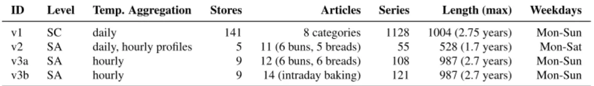
3.2 Datasets . . . 28
3.3 Data Characteristics . . . 30
3.3.1 Hierarchies & Article Clusters . . . 30
3.3.2 Seasonalities . . . 34 3.4 Summary . . . 35 II Forecasting 37 4 Large-scale Forecasting 39 4.1 Introduction . . . 39 4.2 Related Work . . . 40 i
4.2.1 Forecasting using Machine Learning . . . 41
4.2.2 Forecasting on Special Occasions . . . 41
4.2.3 Hierarchical Forecasting . . . 43 4.2.4 Discussion . . . 44 4.3 Methodology . . . 44 4.3.1 Model Scope . . . 45 4.3.2 Regression vs. Classification . . . 46 4.3.3 Additional Remarks . . . 48
4.4 Application: Store-Category Level and Special Days . . . 49
4.4.1 Day Classification . . . 50
4.4.2 Feature Engineering . . . 52
4.4.3 Experimental Setup . . . 53
4.4.4 Results & Discussion . . . 57
4.5 Application: Store-Article Level . . . 67
4.5.1 Experimental Setup . . . 67
4.5.2 Results & Discussion . . . 69
4.6 Application: Hierarchical Forecasts . . . 73
4.6.1 Experimental Setup . . . 74
4.6.2 Results & Discussion . . . 75
4.7 Conclusion . . . 80
III Decision Support 83 5 Daily Decision Support 85 5.1 Introduction . . . 85 5.2 Related Work . . . 89 5.2.1 Demand Uncertainty . . . 89 5.2.2 Demand Substitution . . . 90 5.3 Single-Product Newsvendor . . . 92 5.3.1 Methodology . . . 92 5.3.2 Empirical Evaluation . . . 97
5.4 Multi-Product Newsvendor with Substitution . . . 107
5.4.1 Methodology . . . 108
5.4.2 Empirical Evaluation . . . 111
5.5 Conclusion . . . 119
6 Intraday Decision Support 123 6.1 Baking Plan Generation . . . 123
6.1.1 Introduction . . . 123
6.1.2 Related Work . . . 124
CONTENTS iii 6.1.4 Empirical Evaluation . . . 131 6.1.5 Conclusion . . . 139 IV Wrap-up 141 7 Conclusions 143 7.1 Summary . . . 143
7.2 Practical & Managerial Implications . . . 145
7.3 Future Work . . . 146
List of Tables
3.1 Overview of the feature groups. . . 29
3.2 Overview of the evaluated datasets. . . 29
4.1 Transformation of a regression problem to a classification problem. . . 47
4.2 Classification: 1-hot encoding. . . 47
4.3 Classification: Ordinal encoding. . . 47
4.4 List of public holidays. . . 51
4.5 List of special days. . . 51
4.6 Example for special day features. . . 53
4.7 Statistics on the time series length. . . 53
4.8 Number of observations per special day type. . . 54
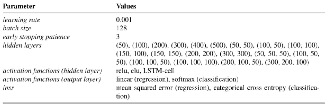
4.9 Evaluated architectures and hyper-parameters for neural networks. . . 55
4.10 Hyper-parameters for LightGBM. . . 55
4.11 Selected architectures and hyper-parameters for neural networks. . . 55
4.12 Results of the evaluation of the baseline and reference methods. . . 58
4.13 Results of the evaluation of the machine learning methods. . . 61
4.14 Comparison ofCL (median)andCL (max): Differences. . . 63
4.15 Comparison ofCL (median)andCL (max): Accuracy. . . 63
4.16 Machine Learning: Effect of re-fitting. . . 66
4.17 Training & test periods for different sample sizes. . . 68
4.18 Forecast accuracy at the store-article level. . . 69
4.19 Effect of re-fitting during the test phase. . . 72
4.20 Forecast accuracy using classification at the store-article level. . . 72
4.21 Classification at the store-article level: Effect of the threshold. . . 73
4.22 (Dis-)aggregation ratio between the levels. . . 75
4.23 Accuracy and key figures at different levels of the hierarchy. . . 77
4.24 Forecast accuracy for hierarchical forecasts. . . 78
5.1 Training & test periods for different sample sizes. . . 97
5.2 Forecast performance of the point predictions (sample size: 1.0). . . 100
5.3 Inventory performance analysis (sample size: 1.0) . . . 102
5.4 Correlation analysis: Costs vs. Accuracy. . . 103
5.5 Inventory performance analysis: Effect of the sample size. . . 106
5.6 Price and cost parameters for buns. . . 112
5.7 Price and cost parameters for breads. . . 112
5.8 Substitution rates of buns. . . 112
5.9 Substitution rates of breads. . . 113
5.10 Average proportion of demand of each product within each category. . . 113
5.11 Forecast performance of the point predictions. . . 114
5.12 Average profit and resulting fill rates. . . 116
5.13 Average profit and resulting fill rates under fill rate constraints. . . 120
6.1 Example of a baking plan. . . 123
6.2 Performance analysis of daily forecasts. . . 134
6.3 Performance analysis of hourly profile forecasts. . . 134
6.4 Performance analysis of hourly forecasts. . . 135
6.5 Scheduling: Operational performance. . . 136
6.6 Scheduling: Number of jobs. . . 138
6.7 Scheduling: Number of jobs per program. . . 138
List of Figures
1.1 Supply chain in the bakery domain. . . 7
1.2 Overview of the Decision Support System. . . 10
2.1 Evaluation: Train-test split. . . 24
2.2 Evaluation: Cross-validation. . . 24
2.3 Evaluation schemes. . . 24
3.1 Hierarchies in the retail domain. . . 31
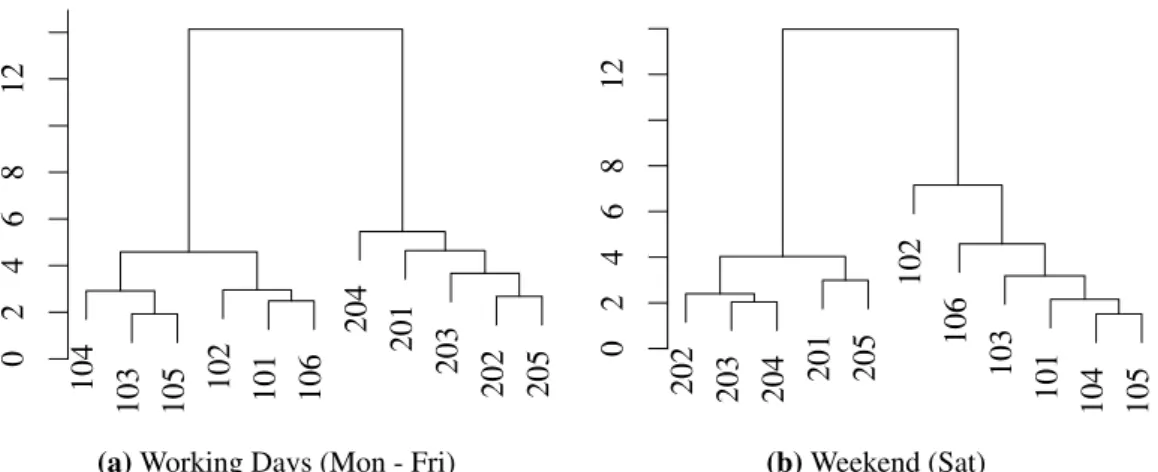
3.2 Hierarchical cluster analysis. . . 33
3.3 Intraday demand profiles. . . 34
3.4 Weekly seasonality of the demand. . . 35
4.1 Illustration of the special day challenge. . . 59
4.2 Comparison of the average rank of the machine learning methods. . . 62
4.3 Multi-step forecast errors at the store-category level. . . 65
4.4 Effect of data usage on the forecast accuracy. . . 70
4.5 Effect of the sample size at the store-article level. . . 70
4.6 Trade-off: Fill rate vs. loss rate. . . 74
4.7 Demand proportions at the store-article level. . . 75
4.8 Accuracy at different levels of the hierarchy. . . 76
5.1 The three levels of data-driven inventory management. . . 86
5.2 The three levels of data-driven inventory management in detail. . . 96
5.3 Forecasts for different service levels using ANN QR. . . 104
5.4 Effect of the sample size (TSL = 0.7). . . 105
5.5 The three levels of data-driven inventory management. . . 108
5.6 Average profit relative to ex-post maximum profit. . . 116
5.7 Average quantities of each product. . . 118
5.8 Average profit with fill rate constraints at category level. . . 119
6.1 Overview on the different phases of our approach. . . 125
6.2 Temporal hierarchy for intraday baking. . . 126
6.3 Demand distributions: Daily and intraday. . . 127
6.4 Illustration of the rolling scheduling approach. . . 131
Part I
Motivation & Foundation
1
Introduction
1.1
Research Motivation
Retailers offering perishable fast-moving consumer goods are required to make hundreds of ordering decisions on a daily basis as they typically run numerous stores and offer a broad assortment. Obviously, determining ordering decisions is a challenging but important task for each retailer as it affects its operational performance. In this section, we provide a brief overview of the specific challenges and highlight opportunities for improvement that motivate our research.
Characteristics of perishable Goods. Fast moving consumer goods (FMCG) comprise articles that are sold at a high frequency as they are mostly required to fulfill the daily needs (e.g. food, drinks) (Kaiser, 2011). The group of FMCG also includes goods that have a short shelf-life due to the perishable character of the products, which makes regular ordering necessary. van Donselaar et al. (2006) classify items as perishable goods if they have a high rate of deterioration at ambient storage conditions (e.g. vegetables) or an obsolescence date that makes reordering impractical (e.g. newspapers). They report that perishable items have
a 50%higher number of average sales per week and a40% smaller median case pack size
compared to non-perishable items. Thus, they conclude that the time between two orders
is 2.5 times smaller for perishable goods, which indicates that they are rather fast moving
goods. Perishable goods are typically delivered several times per week (van Donselaar et al., 2006) and can only be sold for at most a few days as the freshness of such products decreases rapidly. Hence, items that are not sold in time are waste and have to be discarded, which is a major cost factor. On the other hand, running out-of-stock (OOS) leads to loss of revenue as the customers cannot buy the item they are looking for. A retailer can increase its revenue and profit by increasing the availability of the articles while limiting the waste. A common problem for retailers related to the ordering of fresh food is that the order quantities are often determined by store managers based on their experience (van Donselaar et al., 2006, 2010).
Effects and Causes of Stock-outs. The effect of ordering too much can be quantified as the unsold items of perishable goods are waste and cannot be sold after the shelf-life expires. From a financial point of view, the retailer loses the costs related to the production and deliv-ery of the unsold items and has to pay waste collection fees or donate them to charity. For articles having a small profit margin, it is important to limit avoidable costs. On the other
hand, ordering too little leads to OOS, which is much harder to quantify as the customer re-action is uncertain. Ehrenthal and Stölzle (2013) consider that an article is OOS if it cannot be bought by a customer at a given point in time. Studies suggest that the global average
of OOS is 8.3%(Corsten and Gruen, 2003). OOS leads to an immediate revenue loss of
4%(Gruen et al., 2002) but also affects customer loyalty and jeopardizes future sales (Zinn
and Liu, 2008).
The effects of OOS have been widely investigated (Campo et al., 2000; Gruen et al., 2002; Gruen and Corsten, 2007; Helm et al., 2013). Campo et al. (2000) state that customers switch stores, substitute items, postpone the purchase or do not buy anything if the required item is not available. However, the actual response depends on factors like a pre-shopping agenda, urgency of the purchase, brand loyalty and store prices (Zinn and Liu, 2001). Therefore, OOS leads to lost sales, dissatisfied shoppers and diminishes store loyalty. It also obstructs sales planning as the historic sales data is distorted and does not reflect the actual demand. This affects the forecast accuracy and consequently decisions because of demand underestimation of items that were occasionally sold out in the past as well as to demand overestimation due to substitution effects. These effects are not limited to the directly affected article category. Ehrenthal and Stölzle (2013) report that OOS of fresh goods leads to the highest turnover loss compared to other categories. Hence, decreasing OOS is a possibility to increase revenue.
The described effects of OOS underline that a retailer gains a competitive advantage by avoiding OOS. Thus, understanding the causes of OOS is required as it points to issues that need to be improved in order to achieve a better service level. Ehrenthal and Stölzle (2013) report that the causes for OOS in the retail industry are specific to retailer, store, category and item. However, many researchers identified inefficient store operations (Gruen et al., 2002; Gruen and Corsten, 2007; Ehrenthal and Stölzle, 2013) and not issues in the upstream supply chain (e.g. shortage) as the primary cause for OOS (Aastrup and Kotzab, 2010). They also observed that the article availability decreases on the downstream towards the re-tail shelves. Collaboration and communication between supplier and rere-tailer provoke fewer problems regarding article availability. In an empirical study, Ehrenthal and Stölzle (2013) optimize the flow of goods by simplifying and structuring the tasks for the store personnel and bundling store deliveries and shelf replenishment. After the implementation of these op-erational changes, OOS was mainly caused by erroneous orders instead of fulfillment and replenishment problems.
Decision Support for perishable Goods. Retailers use automated ordering systems for most items. However, it is often the case that orders for perishable items are based on the experience and judgment of the store manager as the systems are not adapted to perishable goods (van Donselaar et al., 2006) which has several drawbacks:
1. The decision process is not transparent, i.e., store clerks in different stores apply dif-ferent rules for difdif-ferent article categories, and the decisions may not be as accurate as desired.
1.1. RESEARCH MOTIVATION 5
2. The manual decision process is often quite time consuming and does not scale. Some store clerks might consider comparable historic data (e.g. sales of previous weeks) as well as various factors like price, promotions, product quality (e.g. based on the origin country) or weather data if such data is available.
3. The skills of the store managers are not consistent across all stores of a retail chain which makes this approach unreliable.
4. Judgmental forecasts are often less accurate and more biased than statistical fore-casts (Fildes et al., 2009; Syntetos et al., 2010, 2016). In particular, if they are not carried out by experts.
Hence, the usage of an automated decision support system that implements the respective decision rules of the store managers leads to a competitive advantage for the retailer as it reduces the workload of the personnel. In addition to that, an improved decision quality has also a significant impact on the operational performance (van Woensel et al., 2007; Ehrenthal and Stölzle, 2013).
Decisions are based on the estimation of future demand, i.e., demand forecasts. Thus, the performance of a supply chain also depends on the accuracy of the demand forecasts (Ade-banjo and Mann, 2000; Ade(Ade-banjo, 2009) which is reflected by the fact that supply chain forecasting is an active field of research (Fildes et al., 2008; Syntetos et al., 2016). A study in the fast moving consumer goods sector reveals increased product availability, lower inventory levels along the supply chain and more effective use of current capital assets as major ben-efits of effective forecasting (Adebanjo and Mann, 2000). van Donselaar et al. (2006, 2010) argue that automated ordering systems should be customized for specific product groups in order to provide more reliable results which motivates research dedicated to decisions support systems for perishable goods.
Advances in Information Technology and Data Analysis. Retailers accumulate very large datasets (e.g. sales history) over the years that can also be enhanced by external information like calendric events (Hofmann and Rutschmann, 2018). Recent advances in information technology and developments in the area of large-scale data analysis provide new opportuni-ties for exploiting the data and optimizing short-term decisions related to perishable goods. The benefits of decision support systems (DSS) (Holsapple and Whinston, 1996; Holsapple and Sena, 2005; Power, 2008) in the context of supply chain management depend on the age of the dependent fact data as its value decreases between the occurrence of the respective business event and the executed action (Hackathorn, 2004; Watson, 2009). Traditional busi-ness intelligence (BI) systems (Chaudhuri et al., 2011) are too slow at gathering data that is relevant for short-term day-to-day decisions (Sahay and Ranjan, 2008; Hahn and Packowski, 2015). However, this is necessary in the context of decision support for perishable goods. Traditional BI systems access the data warehouse rather than the operational databases that are optimized for online transaction processing (OLTP) and contain the most recent data.
This separation was necessary as the requirements of online analytic processing (OLAP) (e.g. filtering, aggregation, drill-down, pivoting) are different from OLTP. Hence, an ETL (extract transform load) process is necessary for replicating the data into the data warehouse that is accessible by BI systems. In the last decade, the developments of database technol-ogy led to in-memory databases that are capable of efficiently handling OLTP as well as OLAP queries (Plattner, 2009; Sikka et al., 2012) based on fine-granular data. Maintaining the data in-memory allows using data structures that are not suitable for disk-based databases and reduces the latency which makes real-time analytics possible. Due to these advantages, in-memory databases become more popular in supply chain management. The largest class of benefits of real-time BI is related to enhanced operational decisions (Sahay and Ranjan, 2008).
Decision support for perishable goods is an application scenario that can be enhanced with a data-driven DSS. In particular, a DSS that supports a retailer at different organiza-tional levels during the planning process by providing demand forecasts as well as decision recommendations is required in order to standardize and optimize the process. Such a DSS needs to access a satisfying amount of historical as well as most recent point-of-sale (POS) data from the operational database in order to apply techniques and methods like pattern recognition, statistical analysis, regression analysis or predictive modeling. Thereby, POS data needs to be aggregated in real-time to the required temporal and organizational level. Hence, all prediction models are able to access the same operational data that contains near real-time information of the sales. Those requirements are met by state-of-the-art technology. To summarize, retailers offering perishable goods can expect various benefits from dedi-cated decision support for such goods (van Donselaar et al., 2006). First, the decision process can be standardized and more transparent. Second, the workload of store managers can be re-duced as decision recommendations are provided by a system. Third, by relying on statistical methods, the quality of the decisions can be improved, which may result in fewer stock-outs as well as less discarded goods. DSSs for perishable goods are not yet universally estab-lished in the retail industry as they are only enabled by advances in information technology in the last decade that allow the support of day-to-day decisions by exploiting a large data foundation containing the most recent information.
1.2
Problem Description
Our research is motivated by the requirements of retailers offering baked goods. More specif-ically, we will focus on the case of an industrialized bakery. Baked goods are classified as daily fresh items that are not only daily ordered but also have a high number of sales (van Donselaar et al., 2006). A major cost factor for baked goods are excessive stock levels that lead to marked down or thrown away items as the shelf-life of baked goods is usually not longer than one day. Daily production and ordering is necessary as the freshness of baked goods decreases rapidly, which allows selling only on the day of production. It is even the
1.2. PROBLEM DESCRIPTION 7
production facility store oven shelf
intraday in-store operations daily production & delivery
Figure 1.1: The figure depicts the typical supply chain in the bakery domain. The goods are produced in a production facility from which the stores are delivered on daily basis. A part of the assortment needs to be further processed in the stores (e.g. baked) and subsequently placed on the shelves.
case that some baked goods are only delivered in a pre-baked state which means that they need to be baked during the day in the stores. The typical supply chain in the bakery domain is depicted in Figure 1.1. This thesis is primarily concerned with the development and per-formance assessment of solution approaches concerning the following short-term operational decisions:
Daily order quantity. The order or production quantity of each article needs to be deter-mined on a daily basis. The lead time for baked goods is only one day, which means that short-term demand estimations are required.
Intraday baking / shelf replenishment. Some goods are not ready for sale when they arrive at the store and need to be baked during the day and consequently placed on the shelves. Hence, a baking plan, which aligns the baking process with the customer demand, needs to be provided to the store clerks.
The characteristics of the supply chain and the considered retailers allow to emphasize the decisions (e.g. order quantities) as the primary influence on the performance. The supply chain is short and quite agile as all important parts of it are operated by the company, i.e., production, distribution and stores. This reduces the barriers of collaboration between dif-ferent parts of the supply chain. For instance, trust is not an issue and unfiltered access to real-time demand information is given to all parties of the supply chain using state-of-the-art information technology in order to make the demand visible. With respect to baked goods, we do also not face the issue of inaccurate inventory levels as the perishability of the goods does not allow to keep inventory (Holweg et al., 2005), i.e., the goods are sold or discarded on the day of production. Hence, challenges like the bullwhip effect (Lee et al., 1997) are very unlikely and can be ignored.
It is also noteworthy that the final products (e.g. buns, breads) are highly perishable while this is not entirely true for the raw materials (e.g. wheat flour, sugar, salt) of baked goods that can be persisted for longer periods. The fact that the lead time of baked goods is only one day enables decision recommendations based on most recent demand observations.
The aforementioned characteristics underline that it is actually possible to execute short-term decision recommendations. Moreover, retailers typically operate numerous stores that offer a comparable assortment within a geographically restricted region and generate a large data foundation.
1.3
Research Questions
This thesis is concerned with data-driven decision support for perishable goods in the retail industry as described in the previous section. Thereby, we consider the complete process from data to decision. Hence, the central question of our research is:
RQ1 How can available data be leveraged in order to support and optimize operational
deci-sions in the present application scenario?
The question is generally relevant from a practical point of view as retailers accumulate large datasets while it is fairly unknown how the data can be exploited to enhance operations and how data usage affects the performance. In order to contribute to the wide-ranging research question RQ1, we address the following more specific research questions:
RQ2 Are data-driven methods for inventory management of perishable goods a viable
alter-native to model-based approaches?
RQ3 Can the typically separated phases of estimation and optimization be integrated into a
single optimization problem?
The choice of order quantities is ultimately an inventory decision. The literature on inventory management mainly assumes specific distributions, which is problematic as neither the type of the demand distribution nor its parameters are known in real-world applications. Hence, we investigate if it is possible to discard such likely imprecise assumptions and rely on large datasets that enable the use of empirical distributions. In this context, we also examine if the integration of the typically separated steps of demand estimation and decision optimization is feasible and reasonable.
RQ4 Has the forecast accuracy of a prediction model a noticeable influence on the
opera-tional performance?
While (point) forecasts are an essential input for operational decisions, they do hardly reflect them. For example, it makes sense to add safety stock for daily order quantities in order to increase the service level. Another example are the intraday decisions that are reflected in baking schedules, which take not only the demand estimations but also other restrictions like the availability of the ovens into account. Consequently, it is possible that the effect of more accurate predictions diminishes in a succeeding optimization step. Moreover, aside from established forecast accuracy measures, we also assess the performance based on other key figures like costs or achieved service level.
1.4. CONTRIBUTIONS & PUBLISHED WORK 9
RQ5 Are Machine Learning methods suitable for retail demand forecasting? What factors
affect the performance of Machine Learning methods?
Business forecasting literature is dominated by statistical time series forecasting models and the results of comparative studies (e.g. Ahmed et al. (2010); Makridakis et al. (2018a)) in-dicate that pure Machine Learning methods are no viable alternative. However, the charac-teristics of our application scenario (e.g. amount of data) should benefit Machine Learning methods compared to (univariate) time series models. We apply Machine Learning methods and identify factors influencing the performance with respect to data availability.
1.4
Contributions & Published Work
By answering the research questions outlined in the previous section, we contribute in many ways to the state of business forecasting, more precisely retail forecasting, and inventory management of perishable goods:
• We present the requirements of decision support for perishable goods in the bakery
industry and propose solution approaches that cover the whole process from data to operational decisions. We also empirically evaluate the proposed solution approaches on real-world datasets.
• We analyze Machine Learning models for large-scale demand forecasting on daily
re-tail data of fast moving goods.
– We show that Machine Learning methods are a viable alternative to statistical
time series models.
– We analyze factors that influence the performance of Machine Learning methods.
– We show that it can be beneficial to model forecasting as a classification problem
rather than a regression problem.
• We connect Machine Learning and Operations Research.
– We incorporate Machine Learning models and inventory management models for
perishable goods. In this regard, we propose data-driven integrated estimation and optimization solution approaches for the single-product newsvendor problem as well as the multi-product newsvendor problem with substitution.
– We show that the initial forecast accuracy has a significant influence on the
oper-ational performance.
– We show that data-driven approaches outperform their model-based counterparts.
The thesis is based on articles that are already published in international journals and a couple of working papers. I have been a major contributor to all of the following papers:
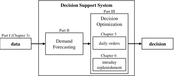
data decision Decision Support System
Demand Forecasting Decision Optimization daily orders intraday replenishment Part I (Chapter 3) Part II Part III Chapter 5 Chapter 6
Figure 1.2:Overview of the Decision Support System.
• J. Huber, A. Gossmann, and H. Stuckenschmidt. Cluster-based hierarchical demand
forecasting for perishable goods.Expert Systems with Applications, 76:140–151, 2017.
• J. Huber, S. Müller, M. Fleischmann, and H. Stuckenschmidt. A data-driven newsvendor
problem: From data to decision. European Journal of Operational Research, 278(3):
904–915, 2019.
• J. Huber and H. Stuckenschmidt. Daily Retail Demand Forecasting using Machine
Learning with Emphasis on Calendric Special Days. Submitted toInternational
Jour-nal of Forecasting (under review), 2018-2019.
• J. Huber and H. Stuckenschmidt. Intraday Shelf Replenishment Decision Support for
perishable Goods.Working Paper (unpublished), 2019.
• S. Müller, J. Huber, M. Fleischmann, and H. Stuckenschmidt. Data-driven Inventory
Management under Customer Substitution.Working Paper (unpublished), 2019.
1.5
Outline
While we formulated the research questions starting from the decisions, the structure of this thesis follows the computational process from data to decision as depicted in Figure 1.2. The thesis is divided into four main parts:
Part I: Motivation & Foundation
The first part provides the motivation and foundations of our research concerningData-driven
Decision Support for perishable Goods. InChapter 1: Introduction(this chapter), we provide a description of the application scenario that is the subject of our research. Additionally, we briefly discuss the challenges and opportunities for improvement that motivate our work and
1.5. OUTLINE 11
lead to the accompanying research questions.Chapter 2: Preliminariescontains a description
of the theoretical and methodical foundations that are the basis of our solution approaches. This predominantly includes time series forecasting and Machine Learning. In addition, eval-uation criteria and evaleval-uation schemes, which we use for the empirical evaleval-uations, are
pre-sented and discussed. InChapter 3: Data Foundation & Characteristics, we give an overview
on the types of data that are typically available to retailers in this application domain and can be used for operational decision support. We also introduce the datasets that are used for the empirical evaluation of our solution approaches and conduct a brief explorative data analysis in order to illustrate prevalent data characteristics.
Part II: Forecasting
We dedicate a self-contained part to demand forecasting (estimation) as this is a crucial input for operational decisions. To this end, we propose approaches to formulate forecasting as a supervised Machine Learning task and exploit the characteristics of the large-scale demand
forecasting scenario (see Chapter 4: Large-scale Forecasting). This includes a
transforma-tion of the regression problem to a classificatransforma-tion problem as well as an identificatransforma-tion of levels of data usage. We conduct a comprehensive empirical evaluation in order to illustrate the viability of Machine Learning.
Part III: Decision Support
After the consideration of data-driven approaches for demand estimation inPart II:
Forecast-ing, we focus on the optimization of daily decisions and intraday decisions as outlined in
the problem description. Consequently, we develop solution approaches for daily decisions inChapter 5: Daily Decision Support. Our methods are based on variants of the
newsven-dor model, which is an inventory management model for perishable goods. InSection 5.3:
Single-Product Newsvendor, we study how data can be exploited for decision optimization
while the daily order quantity of each product is optimized independently. InSection 5.4:
Multi-Product Newsvendor with Substitution, we propose and analyze methods for the joint optimization of order quantities of substitutable products. This is reasonable as high substi-tution rates are observed for baked goods in the event of shortages (e.g. van Woensel et al.
(2007)). Chapter 6: Intraday Decision Supporttargets the last step of the considered bakery
supply chain that is relevant for a subset of the assortment. Therefore, we develop a method for the generation of baking plans based on daily and intraday demand forecasts.
Part IV: Wrap-up
We conclude the thesis inChapter 7: Conclusionsby revisiting our central research questions
(see Section 1.3) and summarizing the key results of the presented research. We also briefly discuss practical and managerial implications of our work. Finally, we outline promising future research directions that extend or enhance our research.
2
Preliminaries
In this chapter, we provide a description of the theoretical and methodical foundations that are the basis of our solution approaches. This includes time series forecasting (see Section 2.1) and Machine Learning (ML) (see Section 2.2). In addition, we present and discuss evaluation criteria and evaluation schemes that we use for the empirical evaluation (see Section 2.3).
2.1
Time Series Forecasting
Retailers make many operational decisions based on forecasts that are calculated by time series forecasting methods (see Section 4.2 and Part III). Generally, time series forecasting is concerned with the prediction of the next values, or even the distribution of the next values,
of a sequence of uniformly spaced time instantsY = (y1, . . . , yn)withyt ∈ R(Hyndman
and Athanasopoulos, 2014). We denote the prediction withyˆt+hwithhbeing the forecasting
step.
2.1.1 Methods
We consider several standard benchmark methods as well as more sophisticated statistical time series models. We focus on methods that explicitly handle seasonal data as the demand of the considered products is subject to a strong weekly seasonality (see Section 3.3). The re-view of De Gooijer and Hyndman (2006) implies that the most popular traditional approaches are exponential smoothing models (Gardner, 1985, 2006) and auto regressive integrated mov-ing average (ARIMA) models (Box and Jenkins, 1976).
2.1.1.1 Baseline Methods
The considered simple baseline methods areS-Naïve, S-MAandS-Median. Those variants
are not only standard benchmarks for time series forecasting but also common in the bakery industry as they are easily understandable and cover the prevalent weekly seasonality. The
length of the seasonality is specified bym, e.g.,m= 7for daily data (Monday - Sunday).
Seasonal-Naïve. The forecast is set to the last observed value from the same part of the season:
S-N a¨ıve: ˆyt+h =yt+h−m (2.1)
Seasonal Moving Average. The seasonal moving average method (S-MA) sets the forecast to an average of the last observations from the same part of the season which is an advantage
compared toS-Naïvethat relies on a single observation. However, we need to setk, which
controls the number of considered values:
S-M A: ˆyt+h = 1 k k X i=1 yt+h−mi (2.2)
Seasonal-Median. The method is an alternative to S-MA as it employs a rolling median instead of a rolling average, which makes this method more robust with respect to outliers:
S-M edian: ˆyt+h = median({yt+h−lm|l∈ {1, . . . , k}}) (2.3)
2.1.1.2 Statistical Time Series Models
With respect to statistical methods, we rely on exponential smoothing models and autore-gressive integrated moving average (ARIMA) models. Both model families have shown to perform reasonably well in comparative studies (e.g. Makridakis et al. (2018a)) and are also well-suited for seasonal data.
Seasonal Autoregressive Integrated Moving Average. Autoregressive integrated moving
average (ARIMA) and its seasonal variant S-ARIMA represent a widely used forecasting
method. The autoregressive part (AR) of ARIMA represents a linear combination of past values, while the moving average part (D) is a linear combination of past forecast errors. The time series must be stationary, which can be achieved by differencing (I). The seasonal
model can be specified as ARIMA(p, d, q, P, D, Q)m. Here, p (P) represent the order of
the non-seasonal (seasonal) auto-regressive part, d(D) are the orders of non-seasonal
(sea-sonal) differencing and q (Q) are the order of the non-seasonal (seasonal) moving average
part. Moreover,mstates the periodicity of the time series. The seasonal ARIMA model is
defined as follows:
φ(B)Φ(Bm)(1−B)d(1−Bm)Dyt=µ+θ(B)Θ(Bm)et (2.4)
The operator B is the backshift operator, i.e.,Byt= yt−1, µis a constant andet are error
terms. The auto-regressive (φ(B), Φ(Bm)) and moving average (θ(B), Θ(Bm)) parts are
expressed as polynomials.
φ(B) = 1−φ1B1−φ2B2−. . .−φpBp (2.5)
Φ(Bm) = 1−Φ1B1m−Φ2B2m−. . .−ΦPBP m (2.6)
θ(B) = 1−θ1B1−θ2B2−. . .−θqBq (2.7)
2.1. TIME SERIES FORECASTING 15
Setting the parameters (p,d,q,P,D,Q,m) properly requires statistical knowledge and de-pends on the nature of the data. Hyndman and Khandakar (2008) and Rojas et al. (2008) propose methods that automatically determine the parameters. We rely on an implementa-tion of a method developed by Hyndman and Khandakar (2008) that automatically selects the ARIMA model having the lowest Akaike Information Criterion (AIC) (Akaike, 1974). AIC is a measure for describing the relative quality of a statistical model for a dataset by estimating the information loss and considering the complexity of the model. In order to select the parameters, they use a step-wise approach and traverse the space of possible mod-els in an efficient way until the optimal model is found. In our experiments, we employ the
auto.arima()function from theforecastpackage (Hyndman and Khandakar, 2008)
for the statistical software R (R Core Team, 2017) that implements the approach.
Exponential Smoothing. Exponential smoothing methods calculate the forecast by com-puting a weighted average of past observations. The weights decay as the observations get older. Hyndman et al. (2002, 2008) propose innovation space models that generalize
expo-nential smoothing methods (ETS). The model family comprises30 models that cover
dif-ferent types of errors, seasonal effects and trends (e.g. none, additive, multiplicative). We
use theets()function from theforecastpackage (Hyndman and Khandakar, 2008) for
the statistical software R (R Core Team, 2017) that selects the model with the lowest AIC.
Exemplary, the modelETS(ANA)(additive error term, no trend, additive seasonality) can be
used for many time series in our application scenario. The model can be written in the error correction form that consists of terms for the time seriesyt, the levellt and the seasonality
st. The frequency of the seasonality is controlled bym. The smoothing parametersαandγ
control the effects of the errorset.
yt=lt−1+st−m+et (2.9)
lt=lt−1+αet (2.10)
st=st−m+γet (2.11)
2.1.2 Forecast Uncertainty
The predictions computed by the methods introduced in the previous section are point fore-casts. The forecasts will as frequently underestimate as overestimate the actual demand if the models are correctly specified and unbiased. With respect to decision optimization, it is necessary to consider the uncertainty and the probability distribution related to a forecast. In forecasting literature, the uncertainty of a forecast is considered by density forecasts (Tay and Wallis, 2000) or expressed by prediction intervals (Chatfield, 2001). Prediction intervals describe the range into which a prediction falls with a prescribed probability, while density forecasts provide the probability distribution of the future value. Chatfield (2001) provides
an overview of approaches for calculating prediction intervals. The approaches are generally based on forecast errors:
et+h =yt+h−yˆt+h (2.12)
Thereby, it is important to distinguish between in-sample errors, i.e, errors of one-step pre-dictions in the training set, and out-of-sample forecast errors. The in-sample-errors, which are in fact the difference between the model fit and the actual values, are called residuals. They allow drawing conclusions about the uncertainty of the predicted values. However, they are only comparable with one-step out-of-sample forecast errors as errors accumulate as the forecast horizon increases. The prediction intervals can be calculated with a model dependent formula that typically assumes a standard normal distribution of the forecast errors (Hyndman and Athanasopoulos, 2014). Thereby, the uncertainty related to the model selection, model specification, and parameter estimation is not considered. This often leads to too narrow pre-diction intervals and unsatisfactory results (Chatfield, 2001; Lam and Veall, 2002; De Gooi-jer and Hyndman, 2006). An alternative are re-sampling methods based on empirical errors, which are more computationally intensive but can provide more accurate results (Chatfield, 2001). Fildes et al. (2008) argue that empirical estimates of quantiles are more accurate and that out-of-sample errors are the best estimate for uncertainty. Alternatively, quantile regres-sion allows the direct prediction of a specific quantile of the distribution (Koenker, 2005).
2.1.3 Hierarchical Forecasting
Hierarchical forecasting (Gross and Sohl, 1990) can be applied to exploit the structure of time series data. The main approaches are top-down and bottom-up forecasting. The top-down approach requires forecasting at an aggregate level and allocating the forecasts to the lower level time series (derived forecasts). The bottom-up approach requires forecasting at a lower level and summing the forecasts to obtain the aggregate level forecasts (cumulative forecasts). The applied approach depends on the objective of the forecast. According to Kahn (1998), top-down forecasting is preferred for strategical planning (e.g. budgets) while bottom-up forecasting is preferred for tactical forecasting where detailed forecasts are required (e.g. production and distribution).
2.2
Machine Learning
Machine Learning (ML) methods are by definition able to learn patterns from data without imposing many requirements on the data generating process (Hastie et al., 2009). They are able to learn patterns from data by exploiting large datasets, which makes them suitable for
big data applications. Supervised ML distinguishes between regression andclassification.
The difference is that the target values of a regression problem are quantitative, while the
target values of aclassificationtask are qualitative. In the following, we focus on the problem formulation forregressiontasks as this is the natural problem type for time series forecasting. However, the general concepts are identical for all supervised ML tasks.
2.2. MACHINE LEARNING 17
The general goal is to approximate a function f(·) that models the relation between a
vector (or matrix) of quantitative input variables, calledfeatures,X ∈Rp and a quantitative
output variable, calledtarget,Y ∈R(Hastie et al., 2009).
ˆ
Y =f(X) (2.13)
The predicted value is denoted by Yˆ while the observed value isY. In order to employ
a ML algorithm, we need to provide a (training) datasetD ={(xk, yk)}k=1..nconsisting of
a set of tuples containing featuresxk ∈ Rm that describe a target yk ∈ R. D can also be
expressed as a pair(X,Y)of a feature matrixX∈Rn×pand a target vectorY∈Rn.
Based on the observed training data, a ML algorithm approximates a function f(·) by
minimizing a loss function L(Y, f(x)) that assesses the fit of f(·). A loss function L is
typically a globally continuous and differentiable function, e.g., the squared loss (L2-norm) can be used for regression tasks:
L(Y, f(X)) = (Y −f(X))2 (2.14)
For classification problems, the cross-entropy loss−PK
k=1 gklog(f(x)(k))is typically used as loss function wheregkis a binary indicator for classkandf(x)(k)the predicted probability for classkof the modelf(·)given a feature vectorx.
The parameters θ of f(·) need to be tuned in order to minimize the loss function L.
A common problem is that the approximated function f(·) has a much lower error on the
training dataset Dtrain than on some unseen test dataset Dtest, i.e., it does not generalize
well. This phenomenon is called overfitting. In order to control and prevent that, a validation
dataset Dvalid is usually retained, which can be used to test if the model does overfit the
training dataset.
2.2.1 Time Series Forecasting
Besides traditional methods (see Section 2.1), data-driven approaches like artificial neural networks (ANNs) are also considered for time series forecasting (Zhang et al., 1998; Zhang, 2012). We extend the introduced notion of time series data and forecasting and adapt it to ML. Time series forecasting can be framed as a supervised ML task. In Section 2.1, we introduced a univariate time seriesY = (y1, . . . , yn) withyt ∈ R. Additionally, each data
point yt of a time series Y can be enriched by explanatory variables X = (x1, . . . , xn),
xt ∈ Rp comprising information that is not contained in the original time series but can be
exploited to understand and model the apparent patterns inY. Time series data along with the
explanatory information can be transformed to feature and target pairs that can be processed by a ML algorithm. For instance, a time series(y1, . . . , yn) representing an autoregressive
X= y1 y2 . . . ya .. . ... ... ... yt−a yt−a+1 . . . yt−1 .. . ... ... ... yn−a yn−a+1 . . . yn−1 Y= ya+1 .. . yt .. . yn (2.15)
Hence, the lagged time series observations build the feature matrixX. For the present
appli-cation scenario, each time series is enhanced with explanatory information. Therefore,Xcan
be extended with additional feature data:
X= y1 y2 . . . ya xa+1,1 . . . xa+1,p .. . ... ... ... ... ... ... yt−a yt−a+1 . . . yt−1 xt,1 . . . xt,p .. . ... ... ... ... ... ... yn−a yn−a+1 . . . yn−1 xn,1 . . . xn,p (2.16)
The present modeling is a multiple regression as a single target variable depends on multiple variables covering autoregressive and external information. A ML method can be employed to approximate the functional relation in a data-driven fashion. Thereby, it does not dis-tinguish between the origin of the feature variables, i.e., autoregressive or external, as the semantics are hidden to the method.
2.2.2 Methods
In this section, we briefly introduce ML methods for function (2.13) that we use in this thesis. In particular, we consider ANNs and gradient boosted regression trees. Those types of models have in common that they rely on a gradient-based approach to optimize the model parameters
θ. However, all methods process data in a different way as we outline below.
2.2.2.1 Artificial Neural Networks
ANNs are data-driven models that can approximate any continuous function (Hornik, 1991), making them suitable for forecasting if it is difficult to specify the underlying data generation process. They are mathematical models that are inspired by biological brains and consist of nodes that are connected by weighted edges, which are represented by matrices and vectors. We consider two distinguishable types of ANNs: feed-forward ANNs and recurrent ANNs.
Feed-forward Neural Networks. Feed-forward Neural Networks (FNNs), e.g., a multi-layer perceptron (MLP), are the most popular neural network architecture for time series
forecasting over the last decades (Zhang et al., 1998). In a FNN havingLhidden layers (L≥
2.2. MACHINE LEARNING 19
h(k)(x) =σ(k)(b(k)+W(k)h(k−1)(x)) (2.17)
The output of the input layer is defined as h0(x) = x while the output of the last layer
represents the prediction of the network, i.e.,f(x) =h(L+1)(x). The output of each layer is
connected with a fully connected weight matrixW(k)to the next layer. The input of a layer
gets adjusted with the biasesb(k)of each neuron before it passes an activation functionσ(k).
Recurrent Neural Networks. Recurrent Neural Networks (RNNs) process the input fea-tures in sequential order and apply the same network to each step in a sequence. RNNs maintain an internal memory that allows them to track dynamic patterns. We use a variant of RNNs, called long short-term memory (LSTM) (Hochreiter and Schmidhuber, 1997), which has a sophisticated memory concept based on input gatesit, output gatesot, forget gatesft, and a cell statectthat allows tracking dynamic patterns:
ft=σsigmoid(Wfxt+Ufht−1+bf) (2.18)
it=σsigmoid(Wixt+Uiht−1+bi) (2.19)
ot=σsigmoid(Woxt+Uoht−1+bo) (2.20)
ct=ft◦ct−1+it◦σtanh(Wcxt+Ucht−1+bc) (2.21)
ht=ot◦σtanh(ct) (2.22)
The operator◦ is the Hadamard product, i.e., element-wise multiplication of matrices and
vectors having the same dimension. The parameters of an LSTM unit areW,U, andb.
For both types of ANNs, the input of a node in the network gets passed through an acti-vation function. Thus, we list frequently used actiacti-vation functions:
• logistic function:σsigmoid(x) = 1+1e−x
• hyperbolic function:σtanh(x) = e
x−e−x ex+e−x
• rectified linear activation:σrelu(x) =x+= max(0, x)
• exponential linear activation:σelu(x) =
x ifx≥0
ex−1 otherwise
• linear function:σlinear(x) =x
• softmax function:σsof tmax(x) = [Pexp(x1) cexp(xc). . .
exp(xC) P
cexp(xc)]
While the activation functions of an LSTM cell are specified, this is not the case for FNNs/MLPs, which requires selecting the activation functions during the model building process. In prin-ciple, all activation functions can be used at any layer. For time series forecasting,σlinear(x) is often used at the output layer, but it is also possible to useσrelu(x)to avoid negative
pre-dictions. The activation functionσsof tmax(x) is used for classification and normalizes the
The parameters (weights) of an ANN can be trained with a stochastic gradient-based algorithm. For this purpose, we use the stochastic gradient-based algorithm ADAM proposed by Kingma and Ba (2015). The performance of an ANN also depends on its initial weights, which are randomly set. In order to reduce the variance and to obtain more robust results, we
employ an ensemble of ANNs with themedianensemble operator, as this approach is robust
to the initial weights and provides reliable results (Barrow et al., 2010; Kourentzes et al., 2014).
Bergmeir et al. (2018) show thatk-fold cross-validation is suitable to control overfitting
when ML methods are employed. We employ k-fold cross-validation (Barrow and Crone,
2016; Bergmeir et al., 2018) on the training dataset in order to validate and design the models as the ordering of the observations does not have to be preserved.
ANNs are also able to deal with seasonal time series data. In order to encode a deter-ministic seasonality, we use trigonometric functions as features, as proposed by Crone and Kourentzes (2009). This is a parsimonious approach that requires only two additional input variables per seasonality. Additionally, the approach is non-parametric as no seasonal indices need to be estimated. The two variables arexi,1andxi,2 in periodi, withmrepresenting the
frequency of the seasonality:
xi,1 =sin(2πi/m) (2.23)
xi,2 =cos(2πi/m) (2.24)
2.2.2.2 Gradient Boosted Regression Trees
Decision trees (DTs) are simple binary trees that map an input to the corresponding leaf node. Since the introduction of classification and regression trees, several approaches have been de-veloped that combine multiple DTs for one prediction (e.g. random forest (Breiman, 2001)). Gradient boosted regression trees have gained much interest in recent years and are an
alter-native to ANNs for structured data. The most popular implementations areLightGBM (Ke
et al., 2017a) andxgboost(Chen and Guestrin, 2016). Like any boosting algorithm, they train
a series of simple modelsfk(x)(i.e. decision trees) based on accumulated residuals of the
previous modelL(k)(y,yˆ(k−1)+f
k(x)). Hence, the prediction is the sum of all trained simple modelsfk(x), i.e.,f(x) =PKk=1fk(x).
2.3
Performance Assessment
In this section, we outline and discuss performance measures and evaluation schemes that are used to assess the prediction and decision quality of our solution approaches.
2.3.1 Evaluation Criteria
We rely on established forecast accuracy measures (see Section 2.3.1.1) and additional crite-ria that are more suitable indicators for the assessment of the operational performance (see
2.3. PERFORMANCE ASSESSMENT 21
Section 2.3.1.2). We define all measures based on target valuesy1, . . . , yN and predictions
ˆ
y1, . . . ,yˆN. We can assume that target values (yn) and predictions (yˆn) are larger than zero as we focus on fast moving goods.
We also test if the performance differences are statistically significant. For this purpose, we employ the Wilcoxon signed-rank test (Wilcoxon, 1945) to determine if there are
statis-tically significant differences among the evaluated methods at0.05significance level. It is a
rank-based test that does not require assumptions on the distributions of the key figures. If not stated otherwise, we underline the best performance for each metric and print results that that do not differ from the one of the best method at a significance level of 5% in bold face.
2.3.1.1 Forecast Accuracy
A variety of forecast accuracy measures have been proposed that have different strengths and weaknesses (Hyndman and Koehler, 2006; Hyndman and Athanasopoulos, 2014). The different error measures can be grouped into scale-dependent errors, percentage errors and scaled errors.
Scale-dependent errors include the mean absolute error (MAE) and the root mean square error (RMSE). They are typically used to compare results on datasets having the same units and comparable scales. In general, minimizing the MAE leads to the median while minimiz-ing the RMSE yields the mean (Gneitminimiz-ing, 2011) of the distribution, which is often desired. RMSE penalizes larger errors more than smaller errors in contrast to MAE. An advantage is that both measures are always defined and rather easy to interpret.
M AE= 1 N N X n=1 |yn−yˆn| (2.25) RM SE= r 1 N XN n=1(yn−yˆn) 2 (2.26)
Percentage errors include the mean absolute percentage error (MAPE) and the symmetric mean absolute percentage error (SMAPE). The measures allow the comparison of time series at different scales but are not defined if the target value and/or the prediction is zero. However, this is not an issue with respect to our research as the considered items are sold in rather high quantities every day. Additionally, the mean percentage error (MPE) can be used as a bias indicator as negative and positive errors offset each other.
M AP E = 100· 1 N N X n=1 |yn−yˆn| yn (2.27) SM AP E= 100· 1 N N X n=1 |yn−yˆn| (yn+ ˆyn)/2 (2.28)
M P E= 100· 1 N N X n=1 yn−yˆn yn (2.29)
Scaled errors like the mean absolute scaled error (MASE) (Hyndman and Koehler, 2006) have been introduced as an alternative to percentage-based errors when comparing forecasts on datasets having different scales or units. The absolute forecast errors are scaled based on the error of a simple forecast method, i.e., in our case the seasonal naïve forecast, on the training data. The scaled error is smaller than one if the error of the evaluated method is smaller than the error of the simple reference method on the training data, e.g., the seasonal naïve forecastyˆt=yt−mfor ordered observationsytwith seasonalitym(e.g. m= 7for the weekly seasonality of daily data).
M ASE = 1 N N X n=1 |yn−yˆn| T T−m PT t=m+1|yt−yt−m| (2.30)
In this research, we address the problem of decision support for perishable goods. Thus, the unit of the data is typically the number of items of a specific product which enables the use of MAE and RMSE. However, as we compute the key figures across different stores, we also compute percentage-based errors and scaled errors as the scale of the demand can differ sig-nificantly. By considering different types of error measures, it is less likely that the results are mostly influenced by a small subset of the evaluated time series which makes the results more robust. While other evaluation criteria are available, we selected the aforementioned criteria as they are widely used and easy to interpret. For instance, SMAPE and MASE were used for the evaluation of point forecasts in the recent M4 Forecasting Competition (Makridakis et al., 2018b). Kolassa (2016) highlights that MAE and MASE are not suitable measures for count data and proposes to evaluate the entire predictive distribution rather than single functionals (e.g. mean). However, the study focuses on intermittent demand data instead of fast moving goods that are sold in higher volumes.
2.3.1.2 Operational Performance
In addition to the point forecast accuracy measures, we consider performance metrics that are reasonable indicators for the operational performance of the supply chain. In order to satisfy the customers and to generate revenue, it is important to fulfill a large portion of the demand. Hence, we consider the fill rate (FR) and the service level (SL).
FR = 1− 1 N N X n=1 (yn−yˆn)+ yn (2.31) SL = 1 N N X n=1 I(yn≤yˆn) (2.32)
2.3. PERFORMANCE ASSESSMENT 23
The fill rate is a quantity-based service level as it measures the proportion of the demand that can be fulfilled. The service level (SL) is event-based and indicates the probability that the complete demand can be served. The expected service level for unbiased point forecasts is50%. A higher fill rate and a higher service level is linked to a higher number of items that
have to be discarded. Thus, we also measure the loss (overage) rate (LR).
LR = 1 N N X n=1 (ˆyn−yn)+ yn (2.33)
The overage rate indicates the percentage of goods that need to be discarded in relation to the actual demand. As either the fill rate or the overage rate can be manipulated, we can
sum the deviation from the optimum of both key figures, i.e., (1−FR) + LR. In order to
balance overage and underage, it is necessary to consider costs and apply an asymmetric loss function.
In many cases, the most relevant performance indicator is the actual profit or costs, i.e., deviation from the maximum profit, that are associated with a decision. A decision reflects
the chosen order quantityq for an article having demand d. A retailer sells items for price
p which costc per unit (e.g. production costs). Hence, the retailer bears opportunity costs
or underage costs u = p−c for the unfilled demand, i.e., the chosen order quantity q is
smaller than the demandd. The underage costs can be interpreted as the profit margin of an
item. Contrary, items that are not sold cause overage costso= cif salvage value or waste
management costs are ignored.
Profit =p·max(q, d)−q·o (2.34)
Cost =u·(d−q)+−o·(q−d)+ (2.35)
A general issue with evaluating profits and costs is that exact parameters are hardly known and that long-term effects are difficult to estimate, e.g., customers might switch stores when the demand is frequently not completely fulfilled. Moreover, the point forecast (e.g. expected demand) only maximizes the profit if costs of underestimation and overestimation are equal
(o == u). If this is not the case, the optimal order quantity can be obtained by applying a
newsvendor model (Silver et al., 2017).
2.3.2 Evaluation Schemes
In order to assess the performance of the methods, we need to split an available dataset into a training set and a test set. The training set is used for the selection and training of the models (e.g. fitting the coefficients) while the test set is used to measure the out-of-sample performance. As auto-correlation can be prevalent in time series data, it is important that observations in the test set temporally succeed the training set (see Figure 2.1). Otherwise,
cross-validation (see Figure 2.2) that is frequently used in the context of the evaluation of ML models is not suitable to measure the out-of-sample performance.
Statistical time series models are frequently selected by minimizing an information cri-teria like AIC (Akaike, 1974) (e.g. Hyndman and Khandakar (2008)) which considers the complexity and fit of a model. For ML methods, cross-validation is used for model selection. Hence, the full training set needs to be further split into a training set (i.e. a subset of the full training set) and a validation set. Typically, roughly 80% of the data is used for training and the remaining 20% for testing (Hastie et al., 2009; Hyndman and Athanasopoulos, 2014).
Bergmeir et al. (2018) show thatk-fold cross-validation can be used for selecting ML models
in the context of time series forecasting.
training data test data
time
Figure 2.1:Split of training data and test data. The test data succeeds the training data.
training data test data
k -f o lds ( k =5 )
Figure 2.2:Illustration ofk-fold cross-validation.
training data test data
(a)standard
training data test data
(b)standard (fixed size)
training data test data
(c)fixed train, rolling test
Figure 2.3:Evaluation schemes.
Once the models have been selected, the next step is to determine the out-of-sample per-formance. In general, a rolling-origin evaluation is typically applied in order to increase the robustness of the results. We consider several evaluation schemes as illustrated in Figure 2.3:
Standard The standard approach is to shift the origin of the forecast by one step (e.g. a day) after each prediction (Hyndman and Athanasopoulos, 2014). Thereby, the size of the training set increases as the most recent observation is added to the training set. After each step of the evaluation, the model is trained with all available data.
Standard (fixed size) A small change to the standard approach is to maintain a constant size of the training data. Hence, the oldest observation is discarded as a new observation is added to the training data.
2.3. PERFORMANCE ASSESSMENT 25
Fixed train, rolling test Another alternative is to train the models only on the initial training set, but the evaluation is performed in a rolling-origin fashion. Hence, most recent observations can serve as input for the models, but the models are not trained with those observations.
The standard approach should lead to the most accurate results as the model is frequently trained with all data that is available but this approach is very computationally expensive and might not be feasible in a productive setting for certain types of models. The variant with a fixed training size allows to investigate the effect of the size of the training data on the performance, e.g., some model types might require or benefit more from a larger training set than others. The motivation of the last evaluation scheme is to simulate a more realistic application of the models as it cannot be expected that the models are trained after a new observation becomes available. Hence, the models are not frequently (e.g. daily) trained, but new observations can be used as input for the model. However, if the test set covers a long time span (e.g. several months of daily data), an update of the models (e.g. once a month) can be considered.
When we compare methods in this thesis, we always compare them on the same test set (i.e. empirical observations) and the evaluated methods do only incorporate data that would be available beforehand in a productive application scenario. In some cases, we alter the evaluation schemes in order to highlight characteristics of specific model types, but this is always explicitly mentioned and explained.