Mitigating Algorithmic Bias: Evolving an Augmentation Policy that is Non-Biasing

(1)

Mitigating Algorithmic Bias: Evolving an

Augmentation Policy that is Non-Biasing

Philip Smith

University of North Carolina at Wilmington [email protected]

Karl Ricanek

University of North Carolina at Wilmington [email protected]

Abstract—Artificial Intelligence promises to make the world a safer place through automation. Automobiles can be steered between traffic lines, spoken words can be translated into textual commands, and wanted persons can be identified by law enforcement. These tasks, once only surmountable by humans, can now be performed by AIs with great speed and precision. If these algorithms are negatively biased against certain groups, what unforeseen harm may come to society?

This work focuses on the classification of gender and age, a problem known to have systemic negative bias for certain subgroups, to investigate the role of data augmentation in the mitigation of such bias. A novel approach is proposed for mitigating bias in a deep learning algorithm that estimates age and gender. Settings for numerous data augmentation techniques are learned through an evolutionary process that optimizes data augmentation for specific subgroups. This approach proves to reduce systemic bias while also generalizing models and obtaining results that are state-of-the-art. The tools we use for determining human biometrics must be fair and non-discriminatory. This work examines not only bias, but also the insights gleaned from successful and unsuccessful policies in certain scenarios.

I. INTRODUCTION

Deep learning has proven effective for a wide variety of tasks which were formerly only surmountable by humans. Deep neural networks (DNNs) have been applied to a plethora of emerging technologies such as autonomous vehicles [1], automated content moderation [2], and intrusion detection systems [3]. Many applications of DNNs focus on being able to understand human beings. Studies on sentiment analysis [4], speech recognition [5], and natural language processing [6] demonstrate promising strides towards that goal. Several studies, including face recognition and verification, facial expression analysis, and age and gender classification focus on gleaning details from human faces. While some good results have been reported for the use of deep convolutional neural networks (DCNNs) in the task of age and gender estimation, these works fail to acknowledge that the resultant models are strongly overfit to the characteristics of the dataset. Neural networks are data-driven models, so if the dataset used to train a neural network is biased, then the resultant model will also be biased. Torralba and Efros [7] identify three types of dataset bias and examine cross-dataset results to show how classifier performance can suffer as a result of bias. This algorithmic bias may lead to outcomes that are unfairly inaccurate and/or unrealistic. When considering age and gender estimation, algorithmic bias may arise due to

un-derrepresented subgroups of a population. Certain subgroups may simply be more challenging to identify, and, therefore, would require more data or a more robust model in order to achieve unbiased results. Data augmentation has proven to generalize models while decreasing error by manufacturing more data upon which a model can be trained [8] [9] [10] [11] [12]. Hand-picked data augmentation strategies will sometimes decrease error, but can also lead to an increase in error. Thus, for this work, data augmentation policies are adopted from [13] and an evolutionary algorithm is used to optimize the policies. The application of data augmentation policies has been shown to reduce error by a significant amount, but this can actually worsen the bias ingrained in a model by decreasing error for dataset majorities and increasing error for dataset minorities. As such, in this approach, data augmentation policies are evolved to specifically reduce bias. The bias-mitigating poli-cies also result in a reduction of overall error while further generalizing the model.

II. THEDATASETS

Three large face-image datasets were used for this study: IMDB, Wiki, and MORPH-II (hereafterI, W, andM respec-tively). The IMBD and Wiki datasets were assembled by Rothe et al. in 2016 by crawling the IMDB and Wikipedia websites and by crowd-sourcing some gender labels [14]. MORPH-II is a collection of 55,134 mugshots assembled by Ricanek et al. starting in 2006 [15]. A fourth dataset, the PPB (Pilot Parliments Benchmark) dataset, is used as a final examination of gender bias and is never included in the training validation data. PPB is a collection of 1270 gender-labeled images that was assembled by Buolamwini and Gebru in 2017 [16] for the purposes of studying bias in gender classification models. In [16], subjects from six different countries are labeled with gender and a Fitzpatrick skin type1_{. IMDB, Wiki, and}

II are labeled with age and gender, and MORPH-II is additionally labeled with race. The IMDB and Wiki datasets were cleaned by using a face detector2 _{to locate}

images where only one face was detected with a face score of higher than 70%. The mean face width and height for

1_{Fitzpatrick skin types range from 1-6 where 1 is the fairest skin tone and} 6 is the darkest.

2_{The face detector is a MobileNet-V2 model that was trained on the WIDER} FACE dataset [17]. It is available at https://github.com/yeephycho/tensorflow-face-detection.

(2)

MORPH-II was calculated to be width W = 113.48px and heightH = 130.86px using the corners of the bounding boxes output by the face detector. All IMDB-Wiki faces were resized to the II mean using algorithm 1. Most MORPH-II images have a width and height of 200x240, so all face images are cropped down to this size. Hereafter, image width

iw= 200 and heightih= 240.

Algorithm 1: Crop face to mean face size

Result:A face-cropped image.

/* the bounding box corners below are returned by the

face detector */

x_min; y_min x_max; y_max

center_x = x_min+x₂ _max center_y = y_min+y₂ _max face_width = w = x_max - x_min face_height = h = y_max - y_min

/* W and H are defined in section II */ if w_h>_WH then resize_ratio = rr = W/w else resize_ratio = rr = H/h end center_x = rr * center_x center_y = rr * center_y

/* resize the image in the x and y directions by

resize_ratio */

img.resize(rr, rr)

/* crop an image of size iw×ih around the center of

the face */

img.crop(center_x, center_y, (iw,ih))

A pretrained age and gender estimator from [18] was used to identify potentially mislabeled images which were then manually verified, and the images which were clearly mislabeled were deleted. After the datasets were cleaned there were 55,038 images included from MORPH-II, 35,169 from Wiki, and 131,091 from IMDB. These three datasets S are combined to produce a training set Str which comprises 50% of the dataset. The validation and test sets Sva and

Ste comprise 25% each. This scheme was chosen over the usual 80/10/10 train/validate/test splits for two reasons. Firstly, enough validation data needed to be present in order to create the challenge set (section VI). Secondly, this study was not designed to achieve the lowest error rates, but to show how a limited amount of data can be augmented to mitigate the effects of algorithm bias. Subgroups of the dataset can be defined by the image labels. Every subset is a proper subset of

S and|S|= 221,298. Let Gg be the set of all gender labeled images whereg∈ {m, f}.Gmis all male labeled images and

Gf is all female labeled images. Not all dataset images are gender labeled so|S−(Gm∪Gf)|= 2,812.Ddis the set of all age labeled images where d ∈ {x∈Z|0≤x < 10} and ages for each decade are in the range [10d,10(d+ 1)−1], so D2 would consist of all 20-29 year-old subjects. The final

subset isRr which is the set of all race labeled images where

r ∈ {b, w, o} (black, white, and other), and R ⊆ M. The “other” label refers to all MORPH-II images not labeled black or white so Ro = R −(Rb ∪ Rw). In addition to racial bias, error is observed based upon face illumination. A mean

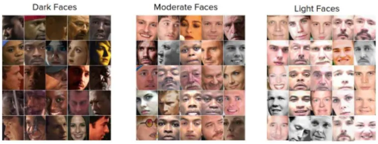
pixel value µ is calculated for the region of the face that exists in 80% of the mean bounding box(WxH). This tighter face crop helps to exclude background and hair. In set B, or face brightness, B0 is the set of all of the darkest faces

with 0 ≤µ < 85, B1 is the set of all moderate faces with

85 ≤ µ ≤ 170, and B2 is the set of all light faces with

170< µ≤255. See figure 1 for examples.

Fig. 1. Separating the dataset by face brightness illustrates the general trend in accuracy by skin tone and also tests the model’s performance in poorly-lit conditions.

III. THEMODEL

The Inception-ResNet-v2 DCNN model was chosen for this project because of its strong ImageNet challenge [19] performance and its relatively lightweight design. Inception-ResNet-v2 combines Google’s Inception modules [8] with Microsoft’s residual connections [20] to yield a 572 weight-layer neural network. Its architecture consists of an input stem which downsamples the image three times before using several stacks of Inception A, B, and C modules, separated by Reduction modules, to extract features before passing them to the final global average pooling and softmax layers. With an age output layer of 100 nodes, and a gender output layer of 2 nodes, both models consist of about 55 million weights and biases. Age models use MAE (mean absolute error) loss while gender models use binary crossentropy loss. Binary crossentropy was chosen for the gender model because training set loss gets very low and a mislabeled or non-cisgender image could disrupt the weights if a higher loss penalty is enforced. All models were trained with the adadelta optimizer [21] because it eliminated the need to tune the learning rate and decay. All input is standardized to the training set mean and standard deviation after data is augmented (in the non-baseline models) but directly before being fed into the network. DLDAE (dynamic label distribution age encoding) [18] is used to encode and decode age labels, and age error is reported as an MAE. As such, all age results are an average error in years. Gender recognition (GR) is interpreted as a binary score. If the gender network output layer node 0 has a value of greater than .5, then it has rendered a prediction of female, otherwise it has predicted male. Gender recognition accuracy is reported in terms of binary accuracy and also as an

F1 score. The F1 score is the harmonic average of precision

and recall, so it is used to more accurately observe the change in model bias. Iftpis a true positive,tnis a true negative,f p

(3)

P = _tp+tpf p and recall C = tp

tp+f n. An F1 score is then

calculated via equation 1.

F1= 2 P C

P+C (1)

IV. BASELINEEXAMINATION

To identify sources of bias, separate models are trained on

Str∩D for age and Str∩G for gender. During training, a randomly selected 1

4 of Svais used as validation data to save

the top 5 models in terms of lowest validation loss. Training is stopped when the model goes for 10 or more epochs with no improvement. All results are reported only on Ste. Sva results are ignored although they are very similar toSte which indicates a lack of validation set overfitting. The cardinality of each subgroup in the test set is shown in table V. As can be seen, some subgroups are severely underrepresented in the dataset and this tends to be the reason for high error. There is an inverse correlation of −0.3222 between Ste subgroup count and age error. An age error standard deviationσis also calculated for each subgroup which shows that estimations can vary wildly for underrepresented subgroups. The Ste MAE overall was 4.62 years – 4.36 for males and 5.13 for females. The results in tables I, II, and IV help identify the greatest sources of age and gender error by subpopulation. In almost every category the baseline models perform better on men than women. This is to be expected since women only comprise 33% of the dataset. Both age and gender models have a difficult time on children and the elderly. The gender recognition model tends to identify boys and young men as women but the reverse is true for the elderly. Faces that are more poorly illuminated are also not as easily identifiable by both the age and gender models. The results for each distinct dataset vary largely as well. The error for MORPH-II is much lower than Wiki and IMDB for a few different reasons. MORPH-II contains no children or elderly past the age of 77, and it was not captured in the wild. Every image is a frontal face image that was taken with camera flash in-front of a neutral background. Wiki is the most challenging dataset because of its lower image count and more frequent facial obstructions. Wiki dataset images tend to be captured by amateur photographers whereas most IMDB photos are taken from movies or shows. It should be noted that the low counts in some categories cause a high standard deviation for error depending on the dataset split.

V. DATAAUGMENTATION

In this instance, the goal of mitigating bias in a trained AI model involves targeting subgroups with high error. Ideally, the error for these subgroups can be decreased without in-creasing the error for other subgroups. A traditional approach to reducing model bias in statistical classifiers like SVMs is to partition the dataset into subgroups that are more balanced [22]. Deep neural networks benefit greatly from being trained on large datasets given their ability to keep generalizing as more examples are seen. As such, a reduction in some of the larger male populations such asD2thoughD4 would not

TABLE I

BASELINERESULTS BYDECADE

Ste∩Gm Ste∩Gf Ste∩Gm Ste∩Gf

Male Female Male Female

Age MAE |σ Age MAE |σ GR Error GR Error

D0 9.24 | 12.35 11.12 | 13.16 27.66% 5.80% D1 3.85 | 6.14 6.43 | 8.35 5.51% 2.83% D2 3.79 | 5.27 4.18 | 5.50 1.47% 1.50% D3 3.70 | 4.98 4.03 | 5.24 1.24% 1.15% D4 4.36 | 5.77 5.96 | 7.52 0.99% 1.67% D5 5.50 | 7.19 8.26 | 10.40 0.75% 3.06% D6 6.24 | 8.41 9.34 | 12.38 0.60% 4.14% D7 8.53 | 10.54 12.77 | 15.62 0.73% 7.45% D8 13.14 | 14.69 15.24 | 17.53 0.00% 4.35% D9 16.94 | 18.17 26.02 | 29.78 0.00% 28.57% TABLE II

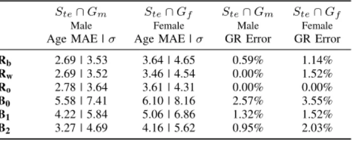
BASELINERESULTS BYRACE ANDILLUMINATION

Rb 2.69 | 3.53 3.64 | 4.65 0.59% 1.14% Rw 2.69 | 3.52 3.46 | 4.54 0.00% 1.52% Ro 2.78 | 3.64 3.61 | 4.31 0.00% 0.00% B0 5.58 | 7.41 6.10 | 8.16 2.57% 3.55% B1 4.22 | 5.84 5.06 | 6.86 1.32% 1.52% B2 3.27 | 4.69 4.16 | 5.62 0.95% 2.03%

result in more robust filters for women, but only less robust filters for men. Since augmenting data has been identified as an efficacious method for virtually increasing the size of a dataset, it can be reasoned that data augmentation techniques could be learned that most effectively augment data for the targeted subgroups. For this experiment, the data augmentation policies from [13] are adopted with some minor improvements. The data augmentations policies in [13] consist of 5 subpolicies with 2 image manipulation techniques per subpolicy. During training, when an image is loaded, a subpolicy is randomly chosen, and its image manipulation techniques are applied.

TABLE III

BASELINERESULTS BYDATASET

M 2.70 | 3.53 3.58 | 4.61 0.52% 0.96%

I 5.07 | 6.80 5.89 | 7.10 1.96% 1.25%

W 5.34 | 7.18 5.25 | 7.88 1.68% 5.99%

TABLE IV BASELINEGENDERSCORES

Ste∩Gm Ste∩Gf

Male Female

Precision 98.55% 98.23%

Recall 99.10% 97.14%

(4)

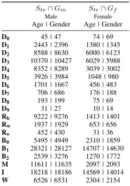
TABLE V TESTSETCARDINALITIES

Ste∩Gm Ste∩Gf

Male Female

Age | Gender Age | Gender

D0 45 | 47 74 | 69 D1 2443 | 2396 1380 | 1345 D2 8588 | 8630 6000 | 6123 D3 10370 | 10427 6029 | 5988 D4 8352 | 8289 3039 | 3002 D5 3926 | 3984 1048 | 980 D6 1701 | 1667 456 | 483 D7 706 | 686 176 | 188 D8 193 | 199 75 | 69 D9 31 | 27 10 | 14 Rb 9222 | 9276 1413 | 1401 Rw 1937 | 1929 653 | 656 Ro 452 | 430 31 | 36 B0 5495 | 4949 2310 | 1859 B1 28321 | 28127 14707 | 14630 B2 2539 | 3276 1270 | 1772 M 11611 | 11635 2097 | 2093 I 18218 | 18186 14569 | 14014 W 6526 | 6531 2304 | 2154

This work applies the evolutionary strategy from [23], rather than the original reinforcement learning technique used in [13], because aging evolution proved to more quickly arrive at near-optimal solutions in a neural architecture search space. The evolutionary algorithm also allows for changes in the number of configurable parameters per data augmentation technique. Rather than using evenly spaced settings for each technique in the policy, this work chooses a set of reasonable defaults to narrow the valid search space. The boundaries and increments for these defaults are based on the results of [13] and also our own prior experimentation with manipulating settings. For example, posterizing image colors down to 3 bits would eliminate most of the features from the image and would not make for good training data, so the posterization technique is limited to 4 bits or higher. The evolutionary algorithm, as opposed to the reinforcement learning strategy, also allows for the expansion and contraction of techniques within a sub-policy. So while the data augmentation policy (DAP) always maintains 5 subpolicies, the number of image manipulation techniques applied by each subpolicy can change. This work also introduces the concept of top-level policies. Some data augmentation techniques have proven to be effective in many other works, so they are considered with a learned probability to be applied to each image after applying a subpolicy. The top-level policies selected for this work are horizontal flipping, mixup [24], cutout [12], and DLDAE. DLDAE is not a form of data augmentation but it is implemented as a top-level policy in order to optimize effective hyperparameters for it. Similar to [13], every data augmentation technique, including the top-level techniques, are applied with a probabilitypwhere

p∈ {0.1x|x∈Z,0< x≤10}except where otherwise speci-fied in table VI. Some of the image manipulation techniques from [13], such as pixel-wise inversion, were not considered because, though they might yield valuable information when

considering images of house numbers, they would not improve the quality of a face-image model. Two new data augmentation techniques are introduced: an improvement to random crop resampling, and a noise robustness technique called random Gaussian tinting. If these techniques did not prove effective then they would be eliminated from subpolicies during the evolutionary process.

A. Random Crop Resampling

Fig. 2. Random cropping witha= 15.

Earlier in the deep learning revolution, image resampling was commonly used as a form of data augmentation [10] [8]. 12-crop resampling, for example, involved taking a crop from each corner of an image, the middle of the image, and resizing the full image down to the target size. Each of these 6 crops would then be flipped horizontally and then all 12 unique images would be fed into the network as training data. Random crop resampling was devised as a way to handle minor discrepancies in image center, scale, and translation all at once. A slight change in a face’s scale should not cause a vastly different age prediction. When random crop resampling is applied, a black border of a width learned using the reasonable defaults seen in table VI encompasses the image. Then, the image is cropped with a random center down to a size that is proportional to, but not necessarily equal to, the input size of the network. Finally, the image is resized to fit the network.

B. Random Gaussian Tinting

Fig. 3. Random Gaussian Tinting witha= 30andb= 5.

In addition to random crop resampling, random Gaussian tinting is introduced as a method of increasing model robust-ness. A small amount of noise on an image should not greatly effect the output of a network; nor should a slight variation in the tint of the image. Random Gaussian tinting works by choosing a subset of the R, G, and B channels, and adding or subtracting a layer of Gaussian noise from those channels. The mean of the Gaussian distribution from which noise is drawn may be shifted by its learnedavalue, and the sampled noise will have a standard deviation of b (see table VI). For example, ifa= 50andb= 5, then the average color channel

(5)

Algorithm 2: Random Crop Resampling

Result:A randomly cropped image.

defrandomly_crop(img, border_width):

img.add_border(border_width, color=black)

/* randomly choose a top-left corner for the crop that will cause it to be larger than or equal

to the target size */

x_min = randint(0, border_width * 2) y_min = randint(0, border_width * 2)

/* ratios to iw and ih of potential crop size from

the top-left corner */

remaining_w_ratio = wr = (iw+border_width∗2)−x_min iw

remaining_h_ratio = hr = (ih+border_width∗2)−y_min ih

width_is_min = wr < hr ? true : false

ifwidth_is_minthen

crop_w =iw+ randint(0,iw+ border_width * 2 - x_min) crop_h = crop_w * ih

iw

else

crop_h =ih+ randint(0,ih+ border_width * 2 - y_min)

crop_w = crop_h * iw ih

end

x_max = crop_w + x_min; y_max = crop_h + y_min img.crop(x_min, y_min, x_max, y_max)

img.resize(iw,ih) return img

shift for the selected channel will be ±50px and the noise standard deviation will be 5px. In this way, if the blue and green channels are selected to be modified, and the sampled noise is added to both layers, then the resultant image will have a teal tint to it and will appear to be of slightly lower quality due to the noise.

VI. THECHALLENGESET

The results of the baseline tests are used to partition a challenge set that contains subgroups that are high in error. As noted earlier, there is a clear gender bias in the baseline models. Children and the elderly tend to be particularly difficult to identify in terms of age and gender, and darker faces also pose a challenge. As such, the challenge set is comprised of validation set images that fit these difficult categories. Only images from Sva are used. During the evolutionary process, the challenge set is used as validation data to evaluate the fitness of the model that’s currently being trained. This forces the algorithm to learn policies that most effectively reduce error specifically for the groups that make up the challenge set. These groups can be seen in table VII. The challenge set contains a total of 5,323 images. 79.8% of the selected images are female. Although the error for males aged 60-79 is relatively high, only 13 of these images are included in

the challenge set and they are randomly drawn for each DAP permutation that is tested to help prevent overfitting.

VII. EVOLVINGDAPS

The first phase of the evolutionary process involves generat-ing and evaluatgenerat-ing a startgenerat-ing population of randomly initialized data augmentation policies. For these policies, between one and three image manipulation techniques are chosen for each subpolicy, and every technique is initialized with settings that are randomly chosen from its reasonable defaults (table

VI). Inception-ResNet-v2 is trained for age estimation for 80 epochs on 11,000 images that are randomly chosen fromStr. The reduced training set size allows models to be trained at a rate of roughly 25 per day using four Tesla V100 video cards. Only age estimation is targeted for bias reduction because it has a larger output vector and is a more challenging problem than gender recognition. The policies learned for gender recognition would probably not transfer well to age estimation because they would allow for stronger data augmentation policies that would make it difficult to recognize age. Each epoch, images are loaded and one subpolicy is applied to each image along with the top-level policies. The challenge set is used as validation data in order to record the lowest loss achieved during training. The validation loss is the fitness score that is used by the evolutionary algorithm to determine which candidate should be mutated. Aging evolution is used as described in [23] which involves recording a population and history of DAPs and their fitness scores. The population has a fixed size of 50. During the evolutionary process, 13

of the population is drawn, and the most fit candidate is chosen to be mutated and evaluated. Three different mutation types are used. The first is a setting mutation where one of the settings for one technique is randomly redrawn from its reasonable defaults. The second is a technique mutation where one technique is chosen to be replaced by a new randomly initialized technique. The third is a size mutation where the number of techniques per subpolicy is increased or decreased. If the subpolicy size is decreased, one of its techniques are simply deleted. If the subpolicy size is in-creased, a new technique is randomly initialized and appended to the subpolicy. The top-level policies are included only in the settings mutation. The average, minimum, and maximum validation losses of the starting population are 0.0141, 0.0122, and 0.0146 respectively. These numbers for the final popula-tion are 0.0092, 0.0086, and 0.0103 which shows a marked decrease in error through evolution. The best discovered policy is illustrated in figure 4. The most commonly chosen data augmentation techniques were random rotation and random Gauss. Random rotation even monopolized an entire subpolicy so, in retrospect, it should probably become a top-level policy. Every data augmentation technique is used at least once which indicates that a wider breadth of techniques is optimal for generalizing models. The bounds on the technique settings are relatively similar for techniques that are chosen more than once. The settings tend to apply mild image manipulations indicating that stronger manipulations make the data unusable. Most subpolicies grew larger in size which rapidly increases the number of potential images that could be generated by a policy.

VIII. RESULTS

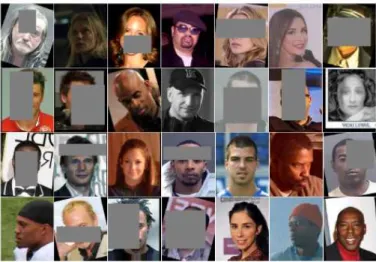
Final models were trained for age and gender using the top five learned augmentation policies. For the final models, while images are being loaded, one of the top five DAPs is chosen for each image. As shown in [13], using more than five DAPs has little further effect on the performance of the model. Figure

(6)

TABLE VI

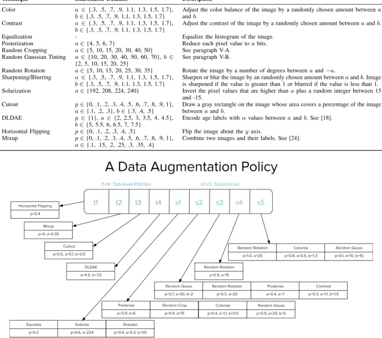
DATAAUGMENTATIONTECHNIQUES

Technique Reasonable Defaults Description

Color a ∈ {.3, .5, .7, .9, 1.1, 1.3, 1.5, 1.7},

b∈{.3, .5, .7, .9, 1.1, 1.3, 1.5, 1.7}

Adjust the color balance of the image by a randomly chosen amount betweena

andb. Contrast a ∈ {.3, .5, .7, .9, 1.1, 1.3, 1.5, 1.7},

b∈{.3, .5, .7, .9, 1.1, 1.3, 1.5, 1.7}

Adjust the contrast of the image by a randomly chosen amount betweenaandb.

Equalization - Equalize the histogram of the image.

Posterization a∈{4, 5, 6, 7} Reduce each pixel value toabits. Random Cropping a∈{5, 10, 15, 20, 30, 40, 50} See paragraph V-A.

Random Gaussian Tinting a∈{10, 20, 30, 40, 50, 60, 70},b ∈ {2, 5, 10, 15, 20, 25}

See paragraph V-B.

Random Rotation a∈{5, 10, 15, 20, 25, 30, 35} Rotate the image by a number of degrees betweenaand−a. Sharpening/Blurring a ∈ {.3, .5, .7, .9, 1.1, 1.3, 1.5, 1.7},

b∈{.3, .5, .7, .9, 1.1, 1.3, 1.5, 1.7}

Sharpen or blur the image by an randomly chosen amount betweenaandb. Image is sharpened if the value is greater than 1 or blurred if the value is less than 1. Solarization a∈{192, 208, 224, 240} Invert the pixel values that are higher thanaplus a random integer between 15

and -15. Cutout p∈{0, .1, .2, .3, .4, .5, .6, .7, .8, .9, 1},

a∈{.1, .2, .3},b∈{.3, .4, .5}

Draw a gray rectangle on the image whose area covers a percentage of the image betweenaandb.

DLDAE p ∈ {1},a ∈{2, 2.5, 3, 3.5, 4, 4.5},

b∈{5, 5.5, 6, 6.5, 7, 7.5}

Encode age labels withαvalues betweenaandb. See [18].

Horizontal Flipping p∈{0, .1, .2, .3, .4, .5} Flip the image about theyaxis. Mixup p∈{0, .1, .2, .3, .4, .5, .6, .7, .8, .9, 1},

a∈{.1, .15, .2, .25, .3, .35, .4}

Combine two images and their labels. See [24].

Fig. 4. This figure represents a data augmentation policy proposed by this work. The top policy learned during evolution is depicted here.

TABLE VII THECHALLENGESET Subgroup Count Gm∩Gf∩D0 114 Gf∩(D1∪D5) 2345 Gf∩(D6∪D7) 625 1 3 Gm∩(D6∪D7) 769 (Gm∩Gf)∩(D8∪D9) 329 (Gf∩Rb)−(Gf∪D0∪D1∪D5∪D6∪D7∪D8∪D9) 1141 Total 5323

5 provides some examples of what training images look like before they are standardized and then fed into the network. The results in tables VIII, IX, and X show that age error is reduced in every single subgroup except for D3 males and

females, and females in the wiki dataset. Age estimation error decreased more forRw than it did forRb suggesting that it is more challenging to recognize the age of black people. This correlates with the face brightness results which indicate that darker faces are much more challenging to recognize even though there is more data available for them than for the light faces. In fact, although B1 is by far the most populous face

(7)

Fig. 5. A random sample of training images with the top 5 data augmentation policies applied.

brightness subgroup, results are best forB2 which is the least

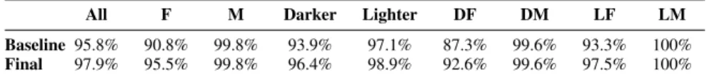
populous subgroup. Overall, MAE went from 4.62 to 4.21 with a final MAE of 4.13 for males and 4.90 for females. The overall gender accuracy went from 98.44% to 98.92%. The gender model was additionally evaluated on the PPB dataset which was held-out during the entire experiment and was not used as training or validation data. Results for PPB are reported in table XII in the same way that they are reported in [16]. The bias-mitigating effect can be seen to improve gender recognition accuracy by 4.7% for females without a decrease in male accuracy. It improved the results for darker-skinned people much more than it did for lighter-skinned people, and the subgroup that showed the most improvement was dark females. Despite these good results, D6 and Rb females in our dataset actually showed an increase in error even though they were included in the challenge set. This indicates that a data augmentation policy may be effectively transferred from age to gender to improve accuracy and mitigate bias, however, to achieve the strongest mitigating effects, the evolutionary algorithm would have to be run again to discover policies that work best for gender.

The final MORPH-II MAE was 2.835 and the gender recognition accuracy was 99.60%. These are the best known results for generalized age and gender estimation models that have not been fine-tuned to overfit the dataset [25] [26].

IX. CONCLUSIONS

The results of this work show that bias in an AI model can be reduced without sacrificing model performance as a whole. In fact, performance increased for almost every single subgroup. State-of-the-art results are obtained for age and gender on the MORPH-II dataset, and results for the IMDB and Wiki datasets are reported for the first time in order to provide an idea of general performance. Running the evolutionary algorithm and evaluating hundreds of models is a computationally expensive process, but further tuning of the DAPs suggested in this paper could result in even

TABLE VIII FINALRESULTS BYDECADE

D0 7.33 | 9.69 8.42 | 10.01 17.02% 5.80% D1 2.82 | 4.79 5.18 | 7.04 2.71% 2.38% D2 3.27 | 4.80 3.77 | 5.23 0.60% 1.37% D3 3.79 | 5.10 4.17 | 5.47 0.78% 1.19% D4 3.86 | 5.40 5.18 | 6.95 0.51% 1.93% D5 5.05 | 6.67 7.18 | 9.51 0.40% 2.86% D6 5.75 | 7.84 7.85 | 10.89 0.30% 4.76% D7 7.29 | 9.54 9.25 | 11.85 0.00% 5.32% D8 11.16 | 13.18 12.03 | 15.46 0.00% 8.70% D9 15.66 | 17.01 17.43 | 19.20 3.70% 28.57% TABLE IX

FINALRESULTS BYRACE ANDILLUMINATION

Rb 2.43 | 3.25 3.35 | 4.42 0.31% 1.36% Rw 2.31 | 3.07 2.82 | 3.78 0.00% 0.91% Ro 2.43 | 3.26 2.85 | 3.63 0.00% 0.00% B0 5.13 | 7.03 5.75 | 7.76 1.36% 3.66% B1 3.48 | 5.44 4.57 | 6.33 0.91% 1.52% B2 2.94 | 4.30 3.67 | 5.17 0.00% 1.69%

better bias-mitigating results. This work shows that DAPs can be transferred from one task to another on the same dataset to reduce bias with some success, however, a deeper exploration into this effect is warranted to understand the dynamics at play. Algorithmic bias should be a standard metric for evaluating data-driven models. It is not enough to report overall performance measures because, as has been proven in the popular press, these metrics do not identify algorithmic bias.

TABLE X FINALRESULTS BYDATASET

M 2.40 | 3.22 3.18 | 4.22 0.27% 1.10%

I 4.62 | 6.38 4.75 | 6.58 1.03% 1.31%

W 4.92 | 6.74 5.50 | 7.46 0.80% 5.25%

TABLE XI FINALGENDERSCORES

Ste∩Gm Ste∩Gf

Male Female

Precision 99.26% 98.25%

Recall 99.12% 98.52%

(8)

TABLE XII PPB GENDERACCURACY

All F M Darker Lighter DF DM LF LM

Baseline 95.8% 90.8% 99.8% 93.9% 97.1% 87.3% 99.6% 93.3% 100%

Final 97.9% 95.5% 99.8% 96.4% 98.9% 92.6% 99.6% 97.5% 100%

REFERENCES

[1] Y. Tian, K. Pei, S. Jana, and B. Ray, “Deeptest: Automated testing of deep-neural-network-driven autonomous cars,” inProceedings of the 40th international conference on software engineering. ACM, 2018, pp. 303–314.

[2] J. Pavlopoulos, P. Malakasiotis, and I. Androutsopoulos, “Deeper atten-tion to abusive user content moderaatten-tion,” inProceedings of the 2017 Conference on Empirical Methods in Natural Language Processing, 2017, pp. 1125–1135.

[3] O. Al-Jarrah and A. Arafat, “Network Intrusion Detection System using attack behavior classification,” in2014 5th International Conference on Information and Communication Systems (ICICS). IEEE, 2014, pp. 1–6.

[4] C. Dos Santos and M. Gatti, “Deep convolutional neural networks for sentiment analysis of short texts,” inProceedings of COLING 2014, the 25th International Conference on Computational Linguistics: Technical Papers, 2014, pp. 69–78.

[5] A. Graves, A.-r. Mohamed, and G. Hinton, “Speech recognition with deep recurrent neural networks,” in2013 IEEE international conference on acoustics, speech and signal processing. IEEE, 2013, pp. 6645– 6649.

[6] K. Hashimoto, C. Xiong, Y. Tsuruoka, and R. Socher, “A joint many-task model: Growing a neural network for multiple nlp many-tasks,”arXiv preprint arXiv:1611.01587, 2016.

[7] A. Torralba and A. A. Efros, “Unbiased look at dataset bias,” inCVPR 2011, June 2011, pp. 1521–1528.

[8] C. Szegedy, W. Liu, Y. Jia, P. Sermanet, S. E. Reed, D. Anguelov, D. Erhan, V. Vanhoucke, and A. Rabinovich, “Going Deeper with Convolutions,” CoRR, vol. abs/1409.4842, 2014. [Online]. Available: http://arxiv.org/abs/1409.4842

[9] L. Taylor and G. Nitschke, “Improving deep learning using generic data augmentation,”CoRR, vol. abs/1708.06020, 2017. [Online]. Available: http://arxiv.org/abs/1708.06020

[10] M. D. Zeiler and R. Fergus, “Visualizing and understanding convolutional networks,” CoRR, vol. abs/1311.2901, 2013. [Online]. Available: http://arxiv.org/abs/1311.2901

[11] H. Zhang, M. Cissé, Y. N. Dauphin, and D. Lopez-Paz, “mixup: Beyond empirical risk minimization,” CoRR, vol. abs/1710.09412, 2017. [Online]. Available: http://arxiv.org/abs/1710.09412

[12] T. Devries and G. W. Taylor, “Improved regularization of convolutional neural networks with cutout,” CoRR, vol. abs/1708.04552, 2017. [Online]. Available: http://arxiv.org/abs/1708.04552

[13] E. D. Cubuk, B. Zoph, D. Mané, V. Vasudevan, and Q. V. Le, “Autoaugment: Learning augmentation policies from data,” CoRR, vol. abs/1805.09501, 2018. [Online]. Available: http://arxiv.org/abs/1805.09501

[14] R. Rothe, R. Timofte, and L. Van Gool, “Dex: Deep expectation of apparent age from a single image,” in Proceedings of the IEEE International Conference on Computer Vision Workshops, 2015, pp. 10– 15.

[15] K. Ricanek and T. Tesafaye, “Morph: A longitudinal image database of normal adult age-progression,” in Automatic Face and Gesture Recognition, 2006. FGR 2006. 7th International Conference on. IEEE, 2006, pp. 341–345.

[16] J. Buolamwini and T. Gebru, “Gender shades: Intersectional accuracy disparities in commercial gender classification,” inConference on fair-ness, accountability and transparency, 2018, pp. 77–91.

[17] S. Yang, P. Luo, C. C. Loy, and X. Tang, “Wider face: A face detection benchmark,” in IEEE Conference on Computer Vision and Pattern Recognition (CVPR), 2016.

[18] P. Smith and C. Chen, “Transfer Learning with Deep CNNs for Gender Recognition and Age Estimation,” in2018 IEEE International Confer-ence on Big Data (Big Data). IEEE, 2018, pp. 2564–2571.

[19] O. Russakovsky, J. Deng, H. Su, J. Krause, S. Satheesh, S. Ma, Z. Huang, A. Karpathy, A. Khosla, M. Bernstein, and et al., “ImageNet Large Scale Visual Recognition Challenge,” International Journal of Computer Vision, vol. 115, no. 3, p. 211–252, Nov 2015.

[20] K. He, X. Zhang, S. Ren, and J. Sun, “Deep Residual Learning for Image Recognition,” CoRR, vol. abs/1512.03385, 2015. [Online]. Available: http://arxiv.org/abs/1512.03385

[21] M. D. Zeiler, “ADADELTA: an adaptive learning rate method,” CoRR, vol. abs/1212.5701, 2012. [Online]. Available: http://arxiv.org/abs/1212.5701

[22] G. Guo and G. Mu, “Simultaneous dimensionality reduction and human age estimation via kernel partial least squares regression,” inCVPR 2011, June 2011, pp. 657–664.

[23] E. Real, A. Aggarwal, Y. Huang, and Q. V. Le, “Regularized Evolution for Image Classifier Architecture Search,”CoRR, vol. abs/1802.01548, 2018. [Online]. Available: http://arxiv.org/abs/1802.01548

[24] H. Zhang, M. Cissé, Y. N. Dauphin, and D. Lopez-Paz, “mixup: Beyond empirical risk minimization,” CoRR, vol. abs/1710.09412, 2017. [Online]. Available: http://arxiv.org/abs/1710.09412

[25] G. Antipov, M. Baccouche, S.-A. Berrani, and J.-L. Dugelay, “Effective training of convolutional neural networks for face-based gender and age prediction,”Pattern Recognition, vol. 72, pp. 15–26, 2017.

[26] R. Rothe, R. Timofte, and L. Van Gool, “Deep expectation of real and apparent age from a single image without facial landmarks,”