6HPLQDU 3DSHU 1Rï ççí
352'8&7,9,7< ',))(5(1&(6
E\
'DURQ $FHPRJOX DQG )DEUL]LR =LOLERWWL
,167,787( )25 ,17(51$7,21$/ (&2120,& 678',(6
6WRFNKROP 8QLYHUVLW\
,661 íêéæðåæçä
6HPLQDU 3DSHU 1Rï ççí
352'8&7,9,7< ',))(5(1&(6
E\
'DURQ $FHPRJOX DQG )DEUL]LR =LOLERWWL
3DSHUV LQ WKH VHPLQDU VHULHV DUH DOVR SXEOLVKHG RQ LQWHUQHW
LQ SRVWVFULSW DQG $GREH $FUREDW õ3')ô IRUPDWVï
'RZQORDG IURP KWWSãîîZZZïLLHVïVXïVHî
6HPLQDU 3DSHUV DUH SUHOLPLQDU\ PDWHULDO FLUFXODWHG WR
VWLPXODWH GLVFXVVLRQ DQG FULWLFDO FRPPHQWï
1RYHPEHU ìääå
,QVWLWXWH IRU ,QWHUQDWLRQDO (FRQRPLF 6WXGLHV
6ðìíç äì 6WRFNKROP
First Version: August 1998 This Version: November 1998
Productivity Di¤erences
¤Daron Acemoglu
yFabrizio Zilibotti
zAbstract
Many technologies used by the LDCs are developed in the OECD economies, and as such, are designed to make optimal use of the skills of these richer countries’ workforces. Due to di¤erences in the supply of skills, some of the tasks performed by skilled workers in the OECD economies will be carried out by unskilled workers in the LDCs. Since the technologies in these tasks are designed to be used by skilled workers, productivity in the LDCs will be low. Even when all countries have equal access to new technologies, this mismatch between skills and technology can lead to sizable di¤erences in total factor productivity and output per worker. Our theory also suggests that productivity di¤erences should be highest in medium-tech sectors, and that the trade regime and the degree of intellectual property right enforcement in the LDCs have an important e¤ect on the direction of technical change and on productivity di¤erences.
JEL Classi…cation: F43, O14, O34, O47.
Keywords: Development, Directed Technical Change, Intellectual Property Rights, Skills, Technology, Total Factor Productivity.
¤We thank Christina Lönnblad, Chris Mazingo and Marcus Salomonsson for technical assistance, and Josh Angirst,
Abhijit Banerjee, John Hassler, Jose V. Rodriguez Mora, Jonathan Temple, Jaume Ventura, and seminar participants at Boston University, Brown, Columbia, IIES and MIT for useful comments. Acemoglu acknowledges …nancial support from NSF Grant SBR-9602116.
yDaron Acemoglu: Massachusetts Institute of Technology, NBER and CEPR. Address: Department of
Economics, E52-371, MIT, 50 Memorial Drive, Cambridge, MA 02142-1347. Ph.: (1) 617 253 1927; fax: (1) 617 253 1330; e-mail: [email protected].
zFabrizio Zilibotti: Institute for International Economic Studies and CEPR. Address: Institute for
Inter-national Economic Studies, Stockholm University, S-106 91 Stockholm, Sweden. Ph.: 46-8-16 22 25; fax: 46-8-16 14 43; e-mail: [email protected]; web page: http://www.iies.su.se/data/home/zilibott/homepage.htm.
I. Introduction
Most economists view technological di¤erences as an important part of the large disparities in per capita income across countries. For example, Paul Romer (1993, p. 543) argues that many nations are poor, in large part, “...because their citizens do not have access to the ideas that are used in industrial nations to generate economic value.” (see also Prescott, 1998). This view receives support from a number of recent studies, such as Klenow and Rodriguez (1997), Caselli et al. (1997), and Hall and Jones (1998), which …nd signi…cant “total factor productivity” (TFP) di¤erences across countries. Large cross-country di¤erences in technology are di¢cult to understand, however. Ideas, perhaps the most important ingredient of technologies, can ‡ow freely across countries, and machines, which embed better technologies, can be imported by less developed countries. This compelling argument has motivated papers such as Mankiw, Romer and Weil (1992), Mankiw (1995), Chari, Kehoe and McGrattan (1997), Parente, Rogerson and Wright (1998) and Jovanovic and Rob (1998) to model cross-country income di¤erences as purely driven by di¤erences in factors rather than in technology.
In this paper, we argue that even when all countries have access to the same set of technologies, there will be large productivity di¤erences among them.1 The center-piece
of our approach is that many technologies used by less developed countries (LDCs/the South) are imported from more advanced countries (the North) and, as such, are designed to make optimal use of the prevailing factors and conditions in these richer countries. To the extent that these conditions are di¤erent in the South, the technologies developed in the North may be inappropriate for the LDCs. For example, the OECD economies prefer to develop new crops suitable for a temperate climate, while many LDCs would be unable to use these and instead need crops suitable to the tropics. Although there are many dimensions in which technological needs of the South di¤er from those of the North, including climate, geography, and culture, we focus on di¤erences in skill scarcity, which we believe to be important in practice. The North is more abundant in skills and tends to develop relatively skill-complementary (skill-biased) technologies, but these are only of limited use to the LDCs.
The main result of our paper is that the mismatch between technologies developed in the North and the skills of the South’s labor force will lead to productivity di¤erences between the North and the South even in the absence of any barriers to technology
1To focus on our mechanism, we abstract from other important determinants of productivity
di¤er-ences. Signi…cant productivity di¤erences across countries may arise due to institutional di¤erences, for example in the degree of property right enforcement, corruption, e¢ciency of the public administration, barriers to technology adoption, agency costs, etc.. See, for example, Parente and Prescott (1994) on barriers to technology adoption, and Acemoglu and Zilibotti (1999) on agency costs.
transfer. The South must use unskilled workers in tasks performed by skilled workers in the North. Since the technologies imported from the North are not suited to the needs of the unskilled workers performing these tasks, the South will have low productivity, even once we control for the contribution of physical and human capital to output. This mismatch between technologies and skills in the South will also naturally amplify the di¤erences in per capita income.
It is also important to investigate whether the di¤erences in productivity and output per worker predicted by our model could be sizeable. Our model gives a simple expression for output per worker as a function of the ratio of capital per worker, ratio of skilled to unskilled workers, and the equilibrium skill-bias in the North’s technology. By considering the U.S. as the North, we perform some back-of-the-envelope calculations. These exercises suggest that the di¤erences predicted by our model are sizeable, and signi…cantly larger than those predicted by a simple “neoclassical” model. More concretely, for example, using cross-country variations in physical and human capital (secondary school attainment), we …nd that the neo-classical model predicts, on average, that output per worker in the LDCs should be approximately 40% of the U.S. while our model predicts the same number to be 23%, much closer to the 21% number we observe in the data. Moreover, our calculations suggest that if technologies were not biased towards the needs of the U.S. economy, output per worker di¤erences would be much smaller. For example, when technologies are appropriate to the needs of the “average” country in our sample, predicted di¤erences in output per worker are reduced by a factor of more than two.
A number of other interesting results also follow from of our analysis. First, the LDCs are predicted to have productivity levels comparable to the OECD countries in very unskilled and very skilled sectors and tasks, but lower productivity in medium skilled tasks. In the most complex tasks, even the very skill-scarce LDCs have to employ skilled workers, who will use the skill-complementary technologies developed in the North and achieve a high level of productivity. In contrast, there will be large productivity di¤erences in sectors where workers are skilled in the North but unskilled in the South, because the technologies are not developed for the unskilled workers in these sectors. This pattern receives some support from the casual observation that there are pockets of e¢cient high-tech industries such as software programming in India.
Second, we show that international trade reduces productivity di¤erences because the LDCs specialize in sectors where technology is appropriate to unskilled workers. Inter-estingly, despite reducing productivity di¤erences, international trade causes divergence in output per worker. Trade reduces the prices of unskilled goods in the North, and dis-courages investment in unskilled technologies, which were those most bene…cial to the South. As a result, trade increases the relative productivity and pay of skilled workers,
and widens the output gap between poor and rich countries. Although other, bene…cial, e¤ects of international trade may be more important in practice, this novel e¤ect of trade on per capita income in the South, via its impact on the skill-bias of new technologies, is also worth bearing in mind.
Third, intellectual property rights emerge as an important determinant of technolog-ical development. When property rights are enforced internationally, …rms in the North have more incentive to develop technologies suited to the South, and output per worker di¤erences decline. However, each less developed country individually bene…ts from not enforcing these rights, creating a potential for a classic Prisoner’s Dilemma.
Finally, our theory suggests a stylized pattern of cross-country convergence in pro-ductivity and GDP. A less developed country diverges from the technological leader when it chooses to use local technologies for which there is no (or little) R&D, but eventually cross-country productivity and income di¤erences tend to become stable as the LDCs start importing the technologies developed in the North. On the other hand, productivity (and income) convergence occurs when a country improves its skill base relative to the North, which concurs with the experiences of Korea and Japan (see for example, Rhee, Ross-Larson and Pursell, 1984; Lockwood, 1968).
The two building blocks of our approach, that most technologies are developed in the North and that these technologies are designed for the needs of these richer economies (directed technical change), appear plausible. For example, over 90% of the R&D expen-diture in the world is carried on in the OECD, and over 35% is in the U.S..2 Moreover,
many recent technologies developed in the North appear to be highly skill-complementary and substitute skilled workers for tasks previously performed by the unskilled (e.g. Katz and Murphy, 1992; Berman, Bound and Machin, 1998). So it should perhaps not be surprising that there are many examples of developing countries, abundant in unskilled workers, which adopt labor-saving technologies requiring specialized technical skills. This has led many development economists, like Frances Stewart (1977, p. xii), to conclude that “...the technology Third World countries get from rich countries is inappropriate”, which is consistent with the approach in this paper.
A number of other papers have emphasized the di¢culties in adapting advanced technologies to the needs of the LDCs. Evanson and Westphal (1995) suggest that new technologies require a large amount of tacit knowledge, which cannot be transferred, slow-ing down the process of technological convergence. The importance of “appropriateness” of technology has also received some attention, for example Salter (1966), Atkinson and Stiglitz (1969) and David (1974). Diwan and Rodrik (1991) use some of the insights of
2Authors’ calculation from UNESCO (1997). UNESCO (1997) gives R&D expenditure as a percentage
this literature to discuss the incentives of Southern countries to enforce intellectual prop-erty rights, as we do in Section V. An important recent contribution to the appropriate technology literature is Basu and Weil (1998), who adopt the formulation of Atkinson and Stiglitz whereby technological change takes the form of learning-by-doing and in‡uences productivity at the capital labor ratio currently in use (see also Temple, 1998). Basu and Weil characterize the equilibrium in a two-country world where the less advanced econ-omy receives productivity gains from the improvements in the more advanced econecon-omy. Our paper di¤ers from Basu and Weil, in particular, and the rest of the appropriate tech-nology literature, in general, in a number of ways. First, what matters in our theory is not capital-labor ratios (as in Atkinson and Stiglitz and Basu and Weil) or size of plants (as in Stewart), but relative supplies of skills, which we believe to be more important in practice. Second, our results do not follow because productivity depends on the ex-act capital-labor or skilled-unskilled labor ratios in use, but because skilled workers use di¤erent technologies than unskilled workers, and in the North skilled workers perform some of the tasks performed by unskilled workers in the South. Third, and perhaps most important, technological change is not an unintentional by-product of production, but a purposeful activity. In particular, R&D …rms in the North direct their innovations to-wards di¤erent technologies depending on relative pro…tability. All our results originate from the fact that the relative abundance of skills in the North induces “skill-biased” in-novations. In this respect, our model is closely related to Acemoglu (1998), which models directed technical change, but primarily focuses on its implications for wage inequality.3
Finally, there is now a large literature on innovation, imitation and technology trans-fer, for example, Vernon (1966), Krugman (1979), Grossman and Helpman (1991), Rivera-Batiz and Romer (1991), Eaton and Kortum (1997) and Barro and Sala-i-Martin (1997). Some of these models, as well as the more traditional models of trade and innovations, such as Krugman (1987), Feenstra (1991) and Young (1991), obtain the result that trade may reduce the growth rate of less developed countries, but the channel is very di¤erent. Moreover, in our model, trade a¤ects TFP and GDP in opposite directions, and a¤ects only relative GDP levels, not long-run growth. The most important di¤erence from our work, however, is that these papers do not analyze an economy in which technological knowledge ‡ows freely across countries, and they do not allow technical progress to be
3We should further note that as is known from trade theory, when there are deviations from factor
price equalization, there will also be factor productivity di¤erences due to di¤erent factor proportions in production. These same forces are present in our economy. But more importantly, directed technical change, the fact that new technologies are developed for the North’s skilled workers, ensures that pro-ductivity in the North is always higher than in the South, and ampli…es the di¤erences in output per worker. Without directed technical change, there is no reason for these factor productivity to be larger in countries with more skilled workers, especially once we control for the direct contribution of physical and human capital to output.
directed towards di¤erent levels of skills.
The plan of the paper is as follows. Section II introduces our basic model and characterizes the equilibrium in the North and the South in the absence of commodity trade and intellectual property rights in the South. Section III shows that productivity is higher in the North than the South and performs some simple back-of-the-envelope calculations to evaluate the potential contribution of our mechanism to the di¤erences in output per worker. Section IV analyzes technical change and productivity di¤erences in a world with commodity trade. Section V analyzes the impact of property rights enforcement in the South on technical change. Section VI endogenizes skill acquisition decisions and shows that improvements in the relative supply of skills in the LDCs lead to productivity convergence, and Section VII analyzes the choice between local and imported technologies in the South. Section VIII concludes, while Appendix A contains the main proofs. Appendix B, which contains some additional results, is available upon request.
II. The Basic Model
A. Countries, Agents and Preferences
We consider a world economy consisting of two groups of countries. There is one large advanced country which we call the North, and a set of small less developed countries which we refer to as the South. To simplify the analysis, we assume all Southern countries to be identical. What distinguishes the North and the South, other than their relative sizes, is the abundance of skills. The North has Hn skilled workers and Ln unskilled workers, whereas the South has Hs skilled workers and Ls unskilled workers. We assume that Hn=Ln> Hs=Ls, so the North is more abundant in skills.
New technologies are developed using …nal output. As we will see shortly, due to a market size e¤ect in the creation of new technologies, countries in the South will per-form no R&D. All technological progress will therefore originate in the North. But the South can adopt these technologies. All consumers have linear preferences given by 1R
0
Ce¡rtdt ;where C is consumption and r is the discount rate, which will also be the interest rate. We suppress time indexes when this causes no confusion.
B. Technology
We …rst describe the production technology which is common across countries, and the R&D technology in the North. To simplify notation, we omit the country indexes for
now. Consumption and investment come out of an output aggregate, C+I+X ·Y ´exp ·Z 1 0 lny(i)di ¸ ; (1)
whereI is investment in machines, andX is expenditure on R&D. We normalize the price
of the consumption aggregate in each period to1. Good i is produced as:
y(i) = "Z NL 0 kL(i; v) 1¡¯dv # ¢[(1¡i)¢l(i)]¯+ "Z NH 0 kH(i; v) 1¡¯dv # ¢[i¢Z ¢h(i)]¯; (2) wherekz(i; v)is the quantity of machines of typevused in sectoritogether with workers of skill levelz (i.e. this is sector and skill-speci…c capital). There is a continuum of machines,
denoted by j 2 [0; NL], that can be used with unskilled workers, and a continuum of machines (di¤erent) j 2 [0; NH] used with skilled workers. Technical progress in this economy will take the form of increases inNL and NH, that is, technical change expands the range of machines that can be used with unskilled and skilled workers. This is similar to the expanding variety model of Romer (1990) (see also Grossman and Helpman, 1991), but allows for technical change to be skill-or labor-complementary as in Acemoglu (1998). Equation (2) also implies that each good can be produced by skilled or unskilled workers, using the technologies suited to their needs. The terms(1¡i)andi imply, however, that
unskilled labor is relatively more productive in producing goods with low indexes. The parameter Z (where Z ¸ 1) enables a positive skill premium. Feasibility requires that R1
0 l(i)di·L and
R1
0 h(i)di·H.
Producers of goodi 2[0;1]take the prices of their products,p(i), wages,wLandwH, and the rental prices of all machines, ÂL(v) and ÂH(v), as given, and maximize pro…ts. This gives the following sectoral demands for machines:
kL(i; v) = h (1¡¯)¢p(i)¢((1¡i)¢l(i))¯=ÂL(v)i1=¯ (3) kH(i; v) = h (1¡¯)¢p(i)¢(i¢Z¢h(i))¯=ÂH(v)i1=¯:
A (technology) monopolist owns the patent for each type of machine. We assume that it also owns machines and rents them out to users at the rental rates Âz(v):
Ma-chines depreciate at the rate ± and investments in machines are reversible. Consider the monopolist owning the patent to a machineº for skill classz, invented at time0. De…ne
the total demand for machine º for skill type z as Kz(º) =R01k(i; º)di: The monopolist
chooses an investment plan and a sequence of capital stocks so as to maximize the present discounted value of pro…ts, as given byVz(º) =R01e¡rt[Âz(º)Kz(º)¡µIz(º)] dt¡µKz0(º); subject to K_z(º) = Iz(º)¡±Kz(º) and to the set of demand constraints given by (3),
where we have suppressed time indexes. µ denotes the marginal cost of machine pro-duction, assumed to be constant; K0
monopolist at the time when the variety º is invented (in this case, at time 0); and
Iz(º) denotes gross investment. Since (3) de…nes isoelastic demands, the solution to this program involves Âz(º) = µ(r+±)=(1¡¯); that is, all monopolists charge a con-stant rental rate, equal to a mark-up over the marginal cost times the interest rate plus the depreciation rate. We assume that the marginal cost of machine production in the North is µ ´ (1¡¯)2=(r +±); so that  = (1¡¯). Pro…t-maximization also implies K0
z(º) =Kz(º) = Kz andIz(º) = ±Kz(º) = ±Kz, that is, each monopolist rents out the same quantity of machines in every period. Notice also that Vz(º) =Vz for allº, that is all machines produced for skill typez are equally pro…table (though this pro…tability can
change over time).
Substituting (3) and the machine prices into (2), we obtain
y(i) =p(i)(1¡¯)=¯¢N
L¢(1¡i)¢l(i) +p(i)(1¡¯)=¯¢NH ¢i¢Z¢h(i):
Therefore, increases in NH (NL) improve the productivity of skilled (unskilled) workers in all sectors. NH and NL are the only state variables of this economy.
R&D (in the North) leads to the discovery of new machine types (blueprints). We assume that technical change is directed, in the sense that the degree to which new tech-nologies are skill-complementary is determined endogenously (see Acemoglu, 1998). Some …rms improve technologies complementing unskilled workers, while others work to invent skill-complementary machines. The cost of discovering a new machine complementing workers of group z (z =L orH) is 1=Áz units of …nal output, so N_z =Á
z ¢Xz where Xz denotes total output devoted to improving the technology of group z. We assume that Áz = Á(xz); Á0 · 0, where xz ´ Xz=Nz, which implies that within a period (i.e., given
Nz) there are constant or decreasing returns to research in the aggregate.
There is a large number of small …rms which can enter to perform R&D for either sector, and each …rm ignores the e¤ect of its expenditure on the productivity of others. More formally, each R&D …rm takes Á(xz) as given when it decides its research expen-diture. A …rm which discovers a new machine becomes the monopolist producer of that machine. We assume Á(xz) = ¡xz¡°; where 0 · ° < 1. This parameterization of the Á function simpli…es the analysis of transitory dynamics.4 We can then write the law of
motion of technologies (new technologies) as:
_
Nz = ¡¢x1z¡° ¢Nz: (4)
Observe that directed technical change is a crucial ingredient in our results; it will enable
4We will focus on the case where° >0. If°= 0, then our balanced growth path results are unchanged,
but there are no transitory dynamics. If we change preferences to Constant Relative Risk Aversion, then there are transitory dynamics even when°= 0, but these are somewhat more complicated.
the North to develop the technologies most suited to its needs, which are di¤erent from those suited to the countries in the South.
C. Analysis
We …rst take the technology variables NL and NH as given and characterize the equilibrium in the North, and we continue to suppress country indexes. We also assume that there is no commodity trade between the North and the South. We start with an intuitive lemma. As with other proofs, the proof of this lemma is in Appendix A.
Lemma 1 There exists J such that for i < J,h(i) = 0 and i > J,l(i) = 0.
In words, all goods with indexes below the threshold J are produced with unskilled
labor, and those with indexes above J are produced with skilled labor only. Using this lemma, we can write the production in sector ias:
y(i) = ( p(i)(1¡¯)=¯¢(1¡i)¢N L¢l(i) if 0·i· J p(i)(1¡¯)=¯¢i¢N H ¢Z¢h(i) if J < i·1 : (5)
Utility maximization, in turn, gives the consumer indi¤erence condition: p(i)y(i) =Y for
alli2[0;1]. These equations enable us to prove:
Lemma 2 In equilibrium,
for any i < J,p(i) =PL¢(1¡i)¡¯and l(i) =L=J;and (6) for anyi > J, p(i) =PH ¢i¡¯and h(i) =H=(1¡J); (7) wherePL and PH are appropriately de…ned price indexes, and
PH PL = µN H NL J 1¡J ZH L ¶¡¯ : (8)
Goods with higher indexes produced with unskilled labor have lower productivity, and command higher prices. The converse is true for skilled goods. Equation (8) is then obtained using the consumer indi¤erence condition. It exploits the fact that goods markets have to clear in the North and the South separately.
To fully characterize the equilibrium for given NL and NH, we must determine J. GoodJ can be produced by either skilled or unskilled workers, and must yield zero pro…t
in either case, thus, wheni=J; both (6) and (7) apply. This implies:
PH PL = µ J 1¡J ¶¯ : (9)
(8) and (9) therefore determine equilibrium relative prices and the threshold sector for a given state of relative technology,NH=NL. Using the fact that the consumption aggregate is the numeraire, we obtain:5
PL = exp(¡¯)¢J¡¯ andPH = exp(¡¯)¢(1¡J)¡¯: (10) Noting that Y = R01p(i)y(i)di; and combining this with (5), (8), (9) and (10), and then simplifying, we obtain a simple reduced form equation for GDP:
Y = exp(¡¯)h(NLL)1=2 + (NHZH)1=2 i2
: (11)
Output per worker is then simply given asY =(L+H). Since wages are equal to marginal
products, we also have:
wH wL =Z µN H NL ¶1=2µZH L ¶¡1=2 : (12)
Finally, notice that combining (12) with (8) and (9), we …nd that the equilibrium share of skilled workers in labor costs is always 1¡J.
D. Technological Progress in the North
We start with the assumption that there are no intellectual property rights in the South, so R&D …rms in the North cannot sell their technologies to Southern …rms. The relevant market for technologies is therefore the North. Since there is no commodity trade, equilibrium R&D in the North can be determined without any reference to the South.
Recalling the above discussion regarding pro…ts of technology monopolists, and using (6) and (7), the return to inventing a new machine for skill class z is:
rVz =¼z+ _Vz; (13) where¼L=¯(1¡¯) (PLn) 1=¯RJ 0 ln(i)di=¯(1¡¯) (PLn) 1=¯ Ln and ¼H = ¯(1¡¯) (PHn) 1=¯R1 J hn(i)di = ¯(1¡¯) (PHn) 1=¯
ZHn are ‡ow pro…ts. Lnand Hn are e¤ectively the “markets” for new technologies, since technology monopolists can only sell machines to Northern producers employing Northern workers. The time derivative captures the fact that Pn
H and PLn may be changing out of the balanced growth path, so that the value of the patent to a certain machine may be di¤erent in the future. Free-entry implies that the value of a technology monopolist must be equal to the marginal cost of innovation, hence¡¡1x¡°
z Vz = 1 at all points in time.6
5That is, we use the normalizationexphR1
0 lnp(i)di
i = 1.
6Notice that if there were a consortium of R&D …rms rather than small ones, we would have (1¡ °)¡¡1x¡°
Along the Balanced Growth Path (BGP), NL and NH must grow at the same rate, thus the same research e¤ort must be allocated to skill- and labor-complementary inno-vations (xL=xH). This is only possible if¼L =¼H (since in BGP, V_L= _VH = 0). Hence, in BGP, we need Pn H Pn L = µZHn Ln ¶¡¯ : (14)
Using (8) and (9), this implies:
NH NL = 1¡J n Jn = ZHn Ln : (15)
This equation uniquely de…nes the relative productivity of skilled and unskilled workers along the BGP as a function of the relative supply of skilled workers in the North. It also determines the threshold sector Jn along the BGP.
The next proposition summarizes this result and the dynamics of the economy outside the BGP in the North.
Proposition 1 There exists a unique and globally (saddle path) stable BGP, given by (9), (10), (12) and (15), and along this growth path, output,NLandNH grow at the rate
g = ¡1=° ¢[exp(¡1)¢¯¢(1¡¯)¢(Ln+ZHn)=r](1¡°)=°:
There is a unique BGP, and starting from anyNL and NH, the economy converges to this BGP. Along this path, a constant fraction of output is devoted to R&D, and the economy grows at the constant rate g. Since both NL and NH grow at the common rate g, the relative productivities of skilled and unskilled workers are constant. Relative
productivities can change along the transition path, however.
As in Acemoglu (1998), an increase in Hn=Ln leads to skill-biased technical change, that is an increase in Hn=Ln raises N
H=NL. The skill premium in the North is always
wn
H=wnL=Z. The skill-biased technical change induced by an increase inHn=Lntherefore exactly cancels the negative direct impact of this variable on relative wages (see eq. (12)).
Finally, we can state the following corollary (proof omitted):
Corollary 1 Let NY ´ Y ¡X and C ´ Y ¡I ¡X: Then, the BGP value of NH=NL (cfr. equation (15)) maximizesNY and C in the North.
Both net output,NY, and consumption,C, are maximized in the BGP, because the
E. Equilibrium in the South
The R&D process speci…ed above entails a market size e¤ect. Since there are no international intellectual property rights, the share of GDP devoted to R&D is an in-creasing function of the country’s market size. To see this, notice that in BGP, free entry implies xc = ¼c=r = [exp(¡1)¢¯¢(1¡¯)¡1¢(r+±)¢µc
¢(Lc+ZHc)=r]1=°, where µc is the marginal cost of machine production in country c (a similar argument also applies
away from the BGP). The share of GDP spent on R&D is therefore an increasing function of Lc +ZHc. Since the South consists of a set of “small” economies, each will have an in…nitesimal market for R&D, and the South, collectively, will not invest in R&D. South-ern producers will instead import all their technologies from the North. More generally, one could also motivate the lack of substantial R&D investments in the South by weak property rights and scarcity of skills.7 Our assumption that each Southern country is
small captures these considerations in a simple way.
To achieve a simple parameterization, we assume that new technologies developed in the North can be adapted in each Southern at some small cost ". Since " > 0, once a
…rm adapts a new technology, it is not pro…table for any others to do so as this would lead to Bertrand competition and negative net pro…ts. Hence, machines in South will also be supplied by a (local) monopolist. However, the marginal cost of machine pro-duction for this local monopolist may be larger than for the inventor, as it does not have access to the inventor’s knowledge base, or because of other distortions. In particu-lar, we assume that the marginal cost of machine production in the South is µs:8 De…ne ½ ´ [µs(r+±)=(1¡¯)2](1¡¯)=¯. Recalling that marginal cost of machine production in
the North isµ ´ (1¡¯)2=(r+±), we have½ ¸ 1: Since this local monopolist also faces
isoelastic demands, machine prices in the South areÂs = (1¡¯)½¯=(1¡¯) =½¯=(1¡¯)Ân. If
½= 1, the same physical to human capital ratios will be used in the South and the North.
In practice, the evidence suggests that the relative price of capital goods is higher in the LDCs (e.g. Jones, 1995), so½ >1 may be more relevant, though this is not necessary for
any of our qualitative results. Equations from subsection C therefore apply with a small modi…cation to introduce½, while NH andNL are still given by R&D in the North as in subsection D. Thus (proof omitted):
7In particular, similar results would be obtained if R&D were performed by skilled workers rather by
using …nal output. In the North,hskilled workers would perform R&D while the remainingH¡hwould work in skilled tasks. With our assumption that each Southern country is small and does not enforce international property rights, the South would once againnot allocate any of its skilled workers to R&D, and we obtain exactly the same results as here. Moreover, with this formulation, even when the South consists of large countries, there will only be limited R&D investments in the South because skilled wages are high. We prefer the speci…cation in the text as it leads to simpler expressions.
8Alternativley, we could assume that the technologu sector in the South is competitive, with cost µs=(1¡¯), with identical results.
Proposition 2 There exists a unique equilibrium in the South where Js is given by 1¡Js Js = µN H NL ZHs Ls ¶1=2 ; (16)
where for alli < Js,h
i = 0andli =Ls=Js, and for alli > Js,li = 0andhi =Hs=(1¡Js), and technologies NH and NL are determined in the North (e.g. given by (15) in BGP). The level of output is:
Ys = exp(¡¯)¢½¡1¢h(NLLs)1=2+ (NHZHs)1=2 i2
(17) Output grows at the same rateg as in the North.
The equilibrium in the South therefore takes a very similar form to that in the North, except that the technology parameters, NH and NL, are taken from the North, and the cost of capital may di¤er (i.e. ½ > 1 is possible). Hence, when the North is in BGP, the South is also in BGP. In particular,Js is constant (thoughJs > Jn), and the growth rate is equal to that of the North,g. The ratio of consumption to GDP is higher in the South,
however, because there is no R&D there.
We can also note that in contrast to Corollary 1, which showed that the North’s net output was maximized, the world’s net output is not maximized. De…ning the world’s net output asNYw ´Yn+Ys¡Xn orCw ´Yn+Ys¡In¡Is¡Xn, we immediately see that neither of these are maximized when NH=NL is at its BGP value given by (15). The reason is that while new technologies developed by the North are appropriate to its needs, they are inappropriate for those of the South.
III. Productivity Di¤erences Between the North and the South
A. Productivity Di¤erences
In this section, we show that in our economy, productivity is higher in the North than in the South, and the mismatch between the technologies of the North and the skills of the South ampli…es the output gap across countries.
First de…ne: A(H; L; NL; NH j ½)´ Y L+ZH = exp(¡¯)¢½ ¡1¢ h (NLL)1=2 + (NHZH)1=2 i2 L+ZH ; y(H; L; NL; NH j ½)´ Y L+H = exp(¡¯)¢½ ¡1 ¢ h (NLL)1=2+ (NHZH)1=2 i2 L+H :
whereY is total output,Ais output per e¢ciency unit of labor, andyis output per worker. We condition on ½ because this variable determines the equilibrium capital labor ratio,
which a¤ects labor productivity. Straightforward di¤erentiation establishes that given
NH=NL,A(H; L; NL; NH j½)is an inverse U-shaped function ofH=Lwith a maximum at
H=L=NH=NL, whereasy(H; L; NL; NH j½)is an inverse U-shaped function ofH=Lwith a maximum at H=L=ZNH=NL:These observations immediately establish the following Proposition (proof omitted):
Proposition 3 Assume that NH=NL is given as in (15), then:
1. A(H; L; NL; NH j ½) is an inverse U-shaped function of H=L with a maximum at Hn=Ln. Hence, for any H=L 6= Hn=Ln, we have A(Hn; Ln; N
L; NH j ½) >
A(H; L; NL; NH j ½).
2. y(H; L; NL; NH j ½) is an inverse U-shaped function of H=L with a maximum at Z2Hn=Ln. Hence, for any H=L < Hn=Ln, we have y(Hn; Ln; N
L; NH j ½) >
y(H; L; NL; NH j ½).
When NH=NL is chosen according to the North’s needs, both output per e¢ciency unit of labor and output per worker are higher in the North than in the South. Moreover, output per e¢ciency unit is maximized in the North, whereas output per worker would be maximized by a skill endowment which is larger than the relative skill endowment in the North (recall thatZ ¸1). Furthermore, bothA(Hn; Ln; N
L; NH j½)=A(H; L; NL; NH j½) and y(Hn; Ln; N
L; NH j ½)=y(H; L; NL; NH j ½), productivity and output per worker in the North relative to the South, are strictly increasing inNH=NL:Hence, as technologies become more skill-biased, the gap in output per e¢ciency unit of labor and output per worker between the North and the South widen. These exercises compare two economies with the same cost of capital ½. It is also immediate that, since ½ = 1 in the North and
½ ¸ 1 in the South, we have A(Hn; Ln; N
L; NH j ½ = 1) > A(Hs; Ls; NL; NH j ½s) and
y(Hn; Ln; N
L; NH j½= 1)> y(Hs; Ls; NL; NH j½s)a fortiori when ½s>1.
Finally, we consider another measure of productivity, TFP, and in the process we attempt to clarify the origins of the productivity di¤erences between the North and the South in our model. Rewrite (5) to obtain:
yL(i) =bL(i)¢KL(i)1¡¯ ¢l(i)¯ and yH(i) =bH(i)¢KH(i)1¡¯ ¢[Z¢h(i)]¯; (18) where thebz(i)’s are the sectoral TFPs given bybL(i) = [(1¡i)¢NL]¯ andbH = [i¢NH]¯; and Kz(i)’s are the sectoral capital stocks given by Kz(i) ´ R0Nzkz(i; v)dº; where z 2 [H; L].9 Lemmas 1 and 2, together with equation (3), imply that Kz(i) = Kz; l(i) = l
9Notice that Z ¢h(i) is the “quantity of human capital” employed in sector i using Z as the
skill-premium. Z should not be part of sectoral TFP, since otherwise sectors and countries with more skilled workers would mechanically have higher TFP.
and h(i) =h: Thus, using (1), we can write total output as: Y = exp ÃZ J 0 lnyL(i)di+ Z 1 J lnyH(i)di ! =B(J; NL; NH)¢ ³ KL1¡¯l¯´J³KH1¡¯(Zh)¯´1¡J (19) whereB(J; NL; NH)´exp ³RJ 0 lnbL(i)di+RJ1lnbH(i)di ´
is aggregate TFP, obtained from separating the terms with factor content from the technology terms. By solving the integral we obtain:
B(J; NL; NH)´ h
NLJNH1¡J(1¡J)¡(1¡J)J¡Ji¯ ¢exp[¡¯]: (20) Notice that (19) factors out skills using the correct factor shares, ¯J for unskilled
workers, and¯(1¡J)for skilled workers, which means that the direct e¤ect of di¤erences in skill supplies on output are already controlled for. (20) therefore does not directly depend onH and L, and TFP di¤erences will not arise in our model due to mismeasurement of the human capital of workers. Also, as the contribution of capital is factored out, TFP does not depend on ½ either. Instead, TFP di¤erences will arise because productivity depends on the threshold sector,J. J determines the extent to which skilled and unskilled
workers are employed in sectors (tasks) for which they may or may not have a comparative advantage. The level of J therefore a¤ects aggregate productivity, and economies with
di¤erent threshold sectors will have di¤erent TFP levels.
Straightforward di¤erentiation establishes that, as with output per e¢ciency unit of labor, TFP is maximized in the North (proof omitted):
Proposition 4 For given NH and NL, B(J; NL; NH) (T F P) is an inverse U shaped functions of J with a maximum at Jm ´ N
L=(NL+NH). Therefore, when NH=NL is given by the BGP equilibrium condition in the North, (15), we have Js > Jn = Jm ´ arg maxB(J; NL; NH).
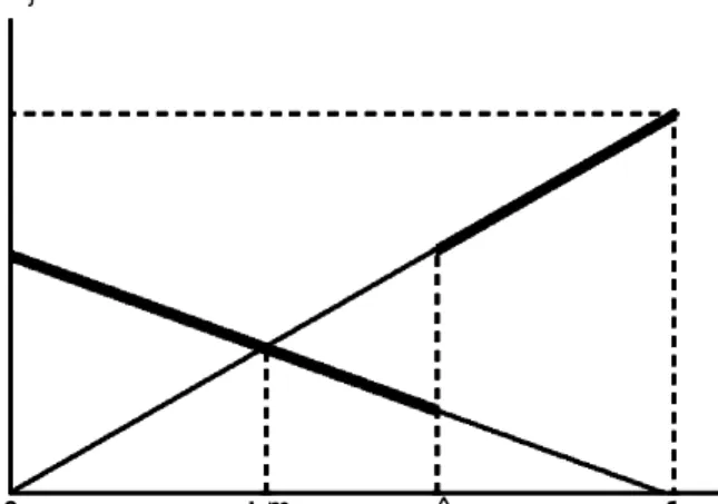
This proposition has an intuitive geometric representation. Figure 1 plots a monotonic transformation of the sectoral TFPs (b(i)1=¯) de…ned in (18). At Jm ´ N
L=(NL+NH); the two schedules cross. Hence, TFP is maximized, when an economy adopts the unskilled technology in all sectorsj· Jm and the skilled technology in all sectors j > Jm. The …g-ure also draws an arbitrary value of the threshold sector,J^, where TFP is not maximized.
SinceJm =Jn, when N
H=NL is chosen by the North, North’s TFP is maximized.
Intuitively, when most R&D is carried out in the North only, and is directed, TFP will be larger in the North than in the South, even though there are no barriers to technology transfer. In particular, as Hs=Ls < Hn=Ln, productivity is larger in the North than in the South, because some sectors in the South employ unskilled workers,
NH NL 0 Jm ^ J 1 j T F Pj1=¯ Figure 1: Sectoral TFP’s.
though productivity would be higher if production were carried out by skilled workers using skilled technologies.10 As we will see in more detail in Section V, if R&D …rms
could sell to Southern producers, they would invest more in unskilled technologies, and productivity in the South would not be as low. Similarly, as noted above, if the South could perform R&D, it would direct it to unskilled machines, and the productivity gap would be smaller. It is therefore the combination of the South importing technologies from the North and directed technical change in the North that leads to the productivity di¤erences between the South and the North.
Proposition 4 has an immediate corollary (proof omitted):
Corollary 2 There are no TFP di¤erences between the North and the South in sector
i for all i · Js or i ¸ Jn. Sectoral TFP is larger in the North than in the South for all
i2 (Js; Jn).
This Corollary can also be illustrated using Figure 1. WhenJs = ^J, sectoral TFPs will be as drawn by thick lines in the …gure. The South is using unskilled workers in sectors
j 2 ³Jm;J^´, where the technologies developed by the North make it more productive to use skilled workers. All productivity di¤erences between the South and the North therefore originate in these “medium-tech” sectors,i 2(Js; Jn). The South concentrates
10Naturally, there is an insu¢cient number of skilled workers in the South to allocate to all tasks
performed by skilled workers in the North. Also, as noted in the introduction, there will be TFP and productivity di¤erences between two economies even in the absence of directed technical change. This can be seen by noting that the productivity di¤erences between the North and the South would arise even for arbitraryNH and NL. However, in this case, the South could have higher TFP, even higher
output per worker, than then North. The novel feature of our model, directed technical change, ensures that the North has higher productivity than the South, as it implies that NH=NL takes the value that
its scarce endowment of skilled workers in a few highly complex tasks. Since technology is common knowledge, in these complex tasks and in the sectors where the North also uses unskilled workers, the South is as productive as the North. The productivity gap emerges instead in those sectors where it is easier to substitute unskilled workers for skilled workers— i.e. those tasks with intermediate i’s. This pattern may explain why India, which has relatively few skilled workers and low productivity compared to the U.S. has a relatively e¢cient software industry, but appears to have low productivity in a range of more traditional industries.
Therefore, overall, because new technologies are developed for the North’s needs, productivity is higher in the North than in the South. A reduction in the degree of skill-bias, which would make technologies more suited to the South’s needs, would reduce the di¤erences in output per worker, output per e¢ciency unit of labor, and TFP between the North and the South.
B. A Simple Quantitative Assessment
In this subsection, we investigate whether the theoretical mechanism we developed could be quantitatively signi…cant. At this point, it is important to note that we are not testing our mechanism, which is an altogether harder task, and a subject for future work. Instead, we simply assess the likely contribution of the mismatch between the technologies of the North and the skills of the South to output per worker di¤erences.
To make our model empirically operational, we need to determine how the ratio of skilled to unskilled workers varies across countries. The skills of importance for our mech-anism are those which facilitate the use of new technologies, such as, computer controlled machines, PCs, automatic retrieval systems, and even perhaps modern organizational forms. In the data, we only observe schooling, however. So, we use four di¤erent mea-sures of “skill” (H=L) to reduce the sensitivity of our results to this partly arbitrary
choice. These are, respectively, the ratio of the population over 25 with at least some primary school attainment to those over 25 with no primary school attainment; the ratio of the population over 25 with at least some secondary school attainment to those over 25 with no secondary school attainment; the ratio of the population over 25 with at least secondary school completion to those over 25 with no secondary school completion; and the ratio of the population over 25 with some higher education to those with none, all from the Barro-Lee data set.11 The second, third and fourth measures may be more
ap-propriate for the skilled-unskilled distinction in our model, since the technologies which can be e¢ciently used by workers with a high school or college would be quite di¤erent
11Web address for Barro-Lee data http://www.worldbank.org/html/prdmg/grthweb/ddbarle2.htm, see
than those appropriate for those with less than high school. Nevertheless, we also look at primary school attainment, which minimizes the cross-country variability in skills, in order to obtain a highly conservative estimate of the di¤erences in the supply of skilled workers between the North and the South.12 We will see below that with all measures, our
model predicts signi…cantly larger variations in output per worker than the neoclassical model.
Table A1 in the Appendix gives the output per worker calculated from the Summers-Heston data set, and our skill measures for a sample of 103 countries.13 As previously
noted by many authors, there are large di¤erences in output per worker across countries. A signi…cant part of this variation is due to di¤erences in physical and human capital per worker, which can be captured by a simple neoclassical model where countries only di¤er in factor endowments. For this reason, we take as our benchmark a neoclassical model where all countries have access to the same technology, as captured byQ, and output is
Cobb-Douglas in total human and physical capital. Then, countryc’s output would be
YNCc =Q¢(Kc)®¢(Lc+ZHc)1¡®:
This is, in fact, the model used by Mankiw, Romer and Weil (1992) and Hall and Jones (1998), among many others, adapted to our environment with two types of workers. We use Kc; Lc and Hc from the data, and set ® = 0:33 (which is equivalent to 1¡¯ in our model), since this is the share of capital in the model. Z is chosen to match the relevant wage premium observed in the U.S.. Given Kc; Lc; Hc; Z and ®; we can calculate the GDP per worker as predicted by the neoclassical benchmark model,y^c
N C, as: ^ yc NC = Yc NC Lc+Hc =Q¢ µ Kc Lc+Hc ¶® ¢ µLc+ZHc Lc+Hc ¶1¡® = = Q¢(½c)¡1 ¢ à KU S Lc+Hc !® ¢ µLc+ZHc Lc+Hc ¶1¡®
whereQ is chosen to normalize y^U S
N C = 1. The second equality follows from the fact that, since½ measures of cost of capital relative to the U.S.,Kc = (½c)¡1=®KU S.
In contrast, our model predicts output per worker,y^c
AZ, to be: ^ ycAZ = Y c AZ Lc +Hc = exp(¡¯)¢(½c)¡1 ¢h(NLLc)1=2+ (NHZHc)1=2 i2 Lc+Hc : (21)
12This is partly motivated by Klenow and Rodriguez (1997)’s critique of Mankiw, Romer and Weil
(1992), which argues that the success of this paper in explaining output per worker di¤erences is due to their use of secondary schooling only.
13Following Hall and Jones (1998), we calculate capital stock in 1985 using the perpetual inventory
method from investment data, and we subtract the contribution of the mining sector from the GDP and the capital numbers, to exclude di¤erences in output per worker caused by di¤erences in natural resource endowments.
where we treat the U.S. as the North, and therefore set NH=NL = ZHU S=LU S, as in equation (15). The level ofNL is set to normalize y^U SAZ = 1.
The relative productivity of skilled workers,Z, in our model corresponds to the skill
premium in the North (see section II.D). In the U.S., the mean earnings of workers with high school attainment (10th grade) or more divided by the mean earnings of workers with no high school attainment (9th grade or less) is over 2, while the mean earnings of full time workers with some college or more divided by the mean earnings of full time workers with no college is approximately 1.75 (all numbers calculated from Current Population Survey of the U.S., 1996). These numbers are quite large, partly due to the fact that in the U.S. relatively few workers have less than 9th grade and the earnings of workers with high school only have been falling. Since choosing a large value of Z ampli…es the
di¤erences in skill endowments across countries, and may overemphasize the importance of our mechanism, we use a range of di¤erent values for Z. We use Z = 1:8as an upper
bound of the relative productivity of skilled workers. We also useZ = 1:5, which we view as a more reasonable estimate of the relative productivity of “skilled” workers, especially when we use secondary school attainment, since the average earnings of those with high school attainment and completion to those with no high school (less than 9th grade) in the U.S. is approximately 1.5. Finally, to check the robustness of the results we also experiment Z = 1, which is clearly implausibly low, as it suggests no skill premium. Nevertheless, even in this case, H-workers use di¤erent technologies than L-workers, and
are more abundant in the North. Therefore, the fact that new technologies developed in the North will be more appropriate to theH-workers will lead to productivity di¤erences, and our mechanism will contribute to output di¤erences. We report this case as a lower bound on the importance of our mechanism.
In Table I, we report three statistics for each experiment, y^LDC, y^5th¡ and <2
s, sep-arately for the neoclassical model and our model. y^LDC denotes the average non-OECD GDP per worker relative to the U.S., andy^5th¡ denotes output per worker relative to the
U.S. in the 5th poorest country in the sample. <2
s, “constrained R2”, is a more general measure of goodness of …t. In particular, letyc denote output per worker from the data and s 2 fNC; AZg, then <2 s = 1 ¡ P c(yc¡ycs) 2 =P(yc)2 is the R2 from a regression
of output per worker in the data on predicted values when we constrain the slope to be equal to 1 and the constant to be 0. <2 would be equal to 1, if there were a perfect …t
between the model and the data, though this measure could also be negative if the …t were particularly bad.
Table I. Output per worker in our model and in the neoclassical model.
Neoclassical model Our model
H=L Z y^LDC N C y^NC5th¡ <2NC y^AZLDC y^AZ5th¡ <2AZ Primary 1.8 0.45 0.16 0.651 0.37 0.06 0.750 Sec. att. 1.8 0.39 0.15 0.816 0.22 0.03 0.936(¤¤) Sec. compl. 1.8 0.39 0.15 0.808 0.24 0.05 0.944(¤¤) Higher 1.8 0.43 0.18 0.718 0.34 0.11 0.881 Primary 1.5 0.46 0.17 0.625 0.37 0.06 0.749 Sec. att. 1.5 0.41 0.16 0.757 0.23 0.03 0.937(¤¤) Sec. compl. 1.5 0.42 0.17 0.745 0.26 0.06 0.940 Higher 1.5 0.45 0.19 0.666 0.36 0.12 0.847 Primary 1.0 0.49 0.21 0.540 0.37 0.06 0.744 Sec. att. 1.0 0.49 0.21 0.540 0.26 0.04 0.935(¤) Sec. compl. 1.0 0.49 0.21 0.540 0.32 0.08 0.903 Higher 1.0 0.49 0.21 0.540 0.42 0.15 0.744
Notes: y^LDCis the predicted average GDP per worker in non-OECD countries andy^5th¡is the predicted
GDP per worker of the 5th poorest country in the sample. In the data,yLDC = 0:21andy5th¡ = 0:03.
H=Lis the relevant ratio of skilled to unskilled workers, and Z is the skill-premium. (*) and
(**) denote that the joint hypothesis a=0 and b=1 in the regression yc=a+byc
s+" cannot be rejected at the 99% and the 90% con…dence levels.
The average output per worker among the non-OECD countries in the sample is about 21% of the output in the U.S., and output per worker in the …fth poorest country is about 1/30th of the U.S. level. The neoclassical model predicts average output among the non-OECD countries to be between 40% and 50%, and output per worker in the …fth poorest country to be between 1/5th and 1/7th of the U.S. level. Like the neoclassical model, our model also underestimates the output gap between rich and poor countries, but much less so. When the skill endowment is measured by secondary school attainment or completion, our model predicts output per worker di¤erences very close to those we observe in practice. For example, with secondary school attainment and Z = 1:5, we obtain y^LDC
AZ = 0:23, or with Z = 1:8, we have y^LDC
AZ = 0:22. Also, in this case our model predicts y^AZ5th¡ = 0:03 for both values of Z. Although in other cases the di¤erences predicted by our model are
less than the di¤erences in the data, these predictions are consistently better than those of the neoclassical model with the corresponding skill measure.
Using our constrainedR2, the neoclassical model also appears to perform reasonably
well, since the di¤erences in physical and human capital are important determinants of output per worker. For example, using secondary school attainment and Z = 1:5, we obtain <2
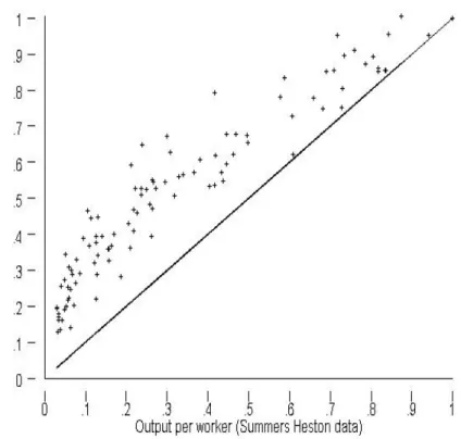
Incorporat-Figure 2: Output per worker: yc
NC vs. yc.
ing the fact that technologies are not appropriate to the LDCs’ needs improves the …t substantially; with secondary school measure and Z = 1:5, the constrained R2 rises to
<2
AZ = 0:94. The improvement is also signi…cant in all other cases, including the most conservative case which minimizes the skill di¤erences between the North and the South by using primary school attainment. Notice also that the results are very robust to dif-ferent values of Z. In particular, the performance of our model remains very good even with Z = 1.14
Figures 2 and 3 plot the output per worker yc and the predicted values from the two models, y^c
N C and y^cAZ. They show, once again, that our mechanism contributes
14We have repeated the calculations in Table I using other measures of skills, for example, primary
and college completion rather than attendance, and using other values ofZ. In all cases, the results are very similar. We have also looked at the performance of the neoclassical model using the measure of average human capital per worker calculated by Hall and Jones (1998), which aggregates workers with di¤erent schooling using di¤erent weights. It is di¢cult to use this measure in our model since there is no distinction between “skilled” and “unskilled” workers with this measure. The results of the neoclassical model with this measure arey^LDC
NC = 0:34, y^5th¡ = 0:10 and<2 = 0:877, thus slightly better than the
numbers for the neoclassical model in Table I, but still substantially worse than our model’s predictions exploiting the equivalent variation.
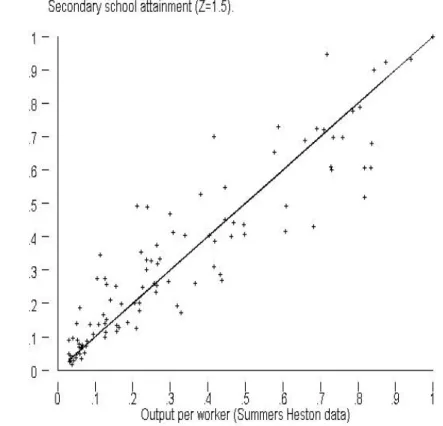
Figure 3: Output per worker: yc
AZ vs. yc: signi…cantly to di¤erences in output per worker (recall that yU S = ^yU S
N C = ^yAZc = 1). In particular, the neoclassical model systematically underpredicts the di¤erences in output per worker between the U.S. and the LDCs (…gure 2), while our model predicts di¤erences in line with those in the data (…gure 3). We therefore conclude that the mismatch between the technologies developed in the North and the skills of the LDCs could be an important factor in explaining the large di¤erences in output per worker and income per capita across countries. In fact, it appears that our mechanism, combined with the physical and human capital di¤erences we observe in practice, could account for a very large fraction of the di¤erences in output per worker in the data.
Finally, to assess the importance of directed technical change in these results, we perform another simple exercise. We calculate yc
ND (where ND stands for no-directed technical change) following equation (21), with the only di¤erences that technologies are now appropriate for the average country rather than for the U.S. That is, we choose
NH=NL =ZH=¹ L¹, whereH=¹ L¹ = (§nc=1Hc=Lc)=nis the (unweighted) average skill
endow-ment of the countries in the sample. With skills measured by secondary school attainendow-ment and Z = 1:5 (the case reported in …gures 2 and 3), we obtain that the average output
per worker in non-OECD countries would be 53% of the U.S. level instead of the 23% predicted by our model above, and the …fth poorest country’s productivity would be 16% of the U.S., as opposed to the prediction of 3% with directed technical change above (and also <2 = 0:26, instead of <2
AZ = 0:94!). Directed technical change is also very impor-tant, using higher education attainment measure, but somewhat less so when skills are measured by primary education attainment.15 These results therefore demonstrate that
directed technical change, which makes new technologies appropriate for the North and not for the South, is crucial for our results. Without this e¤ect, our model would explain substantially less than the simple neoclassical model. These …ndings also suggest that making technologies more appropriate to the needs of the South may be an important step in closing the very large output gaps between rich and poor economies.
IV. Trade and Technology
We now consider a world where all commoditiesi 2[0;1]are traded internationally. We continue to assume that intellectual property rights are not enforced in the South. The main result in this section is that free trade implies productivity convergence, but causes divergence in output per worker.
We use the convention thatHsis the total number of skilled workers in the South and
Ls is the supply of unskilled workers, as well as the supplies in a representative country in the South. Moreover, we normalize½= 1so that the price of capital goods is the same in all countries. International trade implies that commodity prices are equalized in all countries. Since di¤erent commodities can be produced by skilled or unskilled workers only, factor price equalization is always guaranteed. As a result, countries will now adopt the same technology (same thresholdJT). More speci…cally, we have
PT H PT L = à JT 1¡JT !¯ = à NT H NT L ZHw Lw !¡¯=2 ; (22) and wT H wT L =Z à NT H NT L !1=2µ ZHw Lw ¶¡1=2 ;
15With higher education attainment andZ= 1:5, we haveyLDC
ND = 0:52; y
5th¡
ND = 0:21and<2ND = 0:42.
When skills are measured by primary education attainment, we have yLDC
ND = 0:40; yND5th¡ = 0:08 and
<2
ND = 0:71. The reason why directed technical change appears less important with primary attainment
is that most countries in the sample have very high primary attainment (for example, H=L = 249 in
Japan, while onlyH=L = 65 in the U.S.). Thus, the world average H/L is not very di¤erent from the
H/L in the U.S., and directing technical change to the skill endowment of the average country rather than that of the U.S. only makes a small di¤erence. The result changes signi…cantly, if technical change is directed to the endowment of the median country, which is substantially lower than that of the U.S.. In this case, we would have yLDC
ND = 0:48, y
5th¡
N D = 0:13and <2N D = 0:54, signi…cantly worse than the
whereLw =Ls+LnandHw =Hs+Hn are the world supplies,PT
H andPLT are the world prices, and wT
H and wLT are the world wages with free trade.
As patents are not enforced internationally, the balanced growth equilibrium condi-tion, (14), is unchanged; Northern R&D …rms continue to consider Hn and Ln as their markets. Thus, (world) prices have to adjust to satisfy (14). This implies that in the BGP, world relative prices will only depend on the factor endowment of the North:
PT H PT L = à JT 1¡JT !¯ = µZHn Ln ¶¡¯ : (23)
This equation implies that along BGP with trade, world prices and threshold sector,JT, will be equal to those prevailing in the North before trade. However, world prices must also satisfy the world market clearing equation, (22), which now depends on world supplies rather than the supplies of the North only. The state of relative technology therefore has to change. In particular, since the supply of unskilled workers has increased, the relative productivity of skilled workers has to increase to ensure that (23) is satis…ed. More speci…cally, (22) and (23) imply
NT H NT L = µZHn Ln ¶1=2"Hn Ln µHw Lw ¶¡1#1=2 ; (24)
which is larger than the closed economy ratio, since(Hn=Ln)>(Hw=Lw). In other words, trade induces skill-biased technical change.16 More speci…cally, the direction of technical
change depends on the relative market sizes, H=L, and relative prices, pH=pL (recall ¼L and¼H above). Market sizes for technologies do not change, because inventors continue to sell their machines in the North only. But trade, at …rst, increases the relative price of skill intensive goods —i.e. equation (22) at a givenNH=NL. This makes skill-complementary innovations more pro…table and accelerates the creation of skill-complementary machines. In the after-trade BGP, the South, therefore, concentrates its unskilled production in fewer sectors and uses a larger number of skill-complementary machines, while the structure of production in the North reverts back to its pre-trade form. Nevertheless, since technologies are now more skill-complementary, skilled workers have higher relative productivities and wages.
In the next proposition, we characterize how the world economy adjusts to trade opening. To simplify the discussion, we limit our analysis to an unanticipated switch from a world of completely closed economies to one of free trade:
16This possibility was …rst raised by Wood (1994), though without providing a mechanism for it.
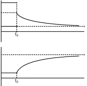
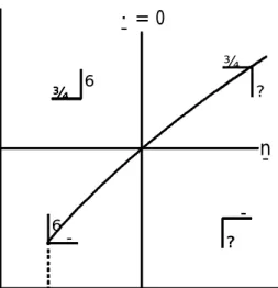
time time t0 t0 (PH=PL)n (PH=PL)Tt0 (PH=PL)s (NH=NL)¤ (NH=NL)n
Figure 4: Dynamics of prices and technology after trade opening.
Proposition 5 Suppose that the relative technologies and prices before trade,(NH=NL)n, relative prices and wages in the North (Pn
H=PLn)n and (wnH=wLn)n, and the equilibrium thresholdsJn andJsare as given by (12), (14), (15) and (16). Consider an unanticipated opening of the world economy to free trade. Then, upon trade opening PH=PL; J and
wH=wL increase in the North and decrease in the South, and are equalized. The system then converges to a new balanced growth path, with (NH=NL)T >(NH=NL)n, while the world price ratio PH=PL decreases to (PH=PL)T = (PH=PL)n and the world threshold sector J decreases to JT = Jn. w
H=wL, the world skill-premium, continues to increase after trade opening and reaches a new level (wH=wL)T > (wH=wL)n. The BGP growth rate of the economy is the same as before trade (g).
The dynamics of prices and technology are described in Figure 4. At the moment the trade regime changes (t0), the level of technology is predetermined at (NH=NL)n. The e¤ects are therefore the same as in the standard trade theory. As the North is more abundant in skills, the relative price of skilled intensive goods and the skill premium increase in the North and fall the South (upper quadrant). What is di¤erent in our theory, however, is the adjustment after this initial response. The change in commodity prices, i.e. the higher level of PH=PL, encourages more skill-complementary innovations, and
NH=NL increases (lower quadrant). The world economy reaches a balanced growth path, as the productivity of skilled workers increases su¢ciently, and the relative price of skill intensive goods return to their pre-trade levels in the North, i.e. (PH=PL)T = (PH=PL)n.
The skill premium in the North increases, not only due to standard trade reasons, but also due to the induced skill-bias technical change.
Since the world relative price of skill intensive goods returns to that of the North before trade, and the North and the South use the same threshold sectorJT, free trade implies that unskilled workers are employed in fewer sectors in the South, i.e. Js falls. Which sectors employ skilled workers in the South, however, is indeterminate as any part of the skilled production could be carried out in the North and imported to the South or vice versa. What is unambiguous is that, overall, the South will import skill-intensive goods and export unskilled goods. Finally, because the market size for new technologies is unchanged and world prices return to those of the North before trade, the long-run growth rate is una¤ected and remains at g.
The next proposition compares GDP and output per worker between the South and the North before and after trade.
Proposition 6 Let Yn be the GDP and yn the output per worker in the North, and Ys the GDP andys in the South before trade. Let YnT and YsT be the GDPs after trade, and
yT
n and ysT be the output per worker after trade. Then, we have YnT=YsT > Yn=Ys and
yT
n=ysT > yn=ys. That is, after trade opening, the GDP and output per worker di¤erences between the North and the South widen.
Trade therefore unambiguouslyampli…es income di¤erences between the South and the North. As we saw above, trade induces new technologies to be further biased towards skilled workers. This reduces the productivity of unskilled workers both in the South and the North, and because the South is more abundant in unskilled workers, its relative situation with respect to the North deteriorates after this change. A number of other papers also obtain the result that trade may lead to more relative inequality among countries (e.g. Krugman (1987), Feenstra (1991) and Young (1991)). Nevertheless, the mechanism in these papers is quite di¤erent from ours. Typically, trade induces less developed countries to specialize in sectors which bene…t less from learning-by-doing than the sectors in which the North specializes. In contrast, in our model, trade changes the direction of technical progress in the North, and leads to larger income di¤erences via this channel. Additionally, in these models trade leads to both TFP and GDP divergence, which is very di¤erent from our result, as we see next:
Proposition 7 Let AT
n and ATs denote after trade output per e¢ciency unit of labor in the North and in the South, respectively, and let BT
n and BsT be TFP. Then, ATn = ATs and BT
n = BsT. That is, after trade opening, di¤erences in output per e¢ciency unit of labor and TFP between the North and the South disappear.17
17If½6= 1, then we would haveAT