Bordo, M. D., Choudhri, E. U., Fazio, G. and MacDonald, R. (2017) The
real exchange rate in the long run: Balassa-Samuelson effects
reconsidered. Journal of International Money and Finance, 75, pp.
69-92. (doi:
10.1016/j.jimonfin.2017.03.011
)
This is the author’s final accepted version.
There may be differences between this version and the published version.
You are advised to consult the publisher’s version if you wish to cite from
it.
http://eprints.gla.ac.uk/141439/
Deposited on: 15 May 2018
Enlighten – Research publications by members of the University of Glasgow
1
The Real Exchange Rate in the Long Run:
Balassa-Samuelson Effects Reconsidered
Michael D. Bordo
Rutgers University, New Jersey Hall, 75 Hamilton Street, New Brunswick,NJ 08901 E-mail: [email protected]
Ehsan U. Choudhri
Department of Economics, Carleton University, Loeb Building 1125 Colonel By Drive, Ottawa, Ontario, K1S 5B6 Canada; E-mail: [email protected]
Giorgio Fazio
Newcastle University Business School, Newcastle University, 5 Barrack Rd, Newcastle upon Tyne, NE1 4SE
E-mail: [email protected]; SEAS, University of Palermo Ronald MacDonald
Adam Smith Business School, Gilbert Scott Building, University of Glasgow, G12 8QQ UK E-mail: [email protected]
Abstract
Historical data for over hundred years and 14 countries is used to estimate the long-run effect of productivity on the real exchange rate. We find large variations in the productivity effect across four distinct monetary regimes in the sample period. Although the traditional Balassa-Samuelson model is not consistent with these results, we suggest an explanation of the results in terms of contemporary variants of the model that incorporate the terms of trade mechanism. Specifically we argue that changes in trade costs over time may affect the impact of productivity on the real exchange rate over time. We undertake simulations of the modern versions of the Balassa-Samuelson model to show that plausible parameter shifts consistent with the behavior of trade costs can explain the cross-regime variation of the productivity effect.
JEL Classification: F41; F31
2
1. Introduction
A basic hypothesis about the behavior of the real exchange rate is that the Purchasing Power Parity (PPP) holds in the long run and the real exchange rate converges to a constant value. Empirical testing of this hypothesis (based on post Bretton Woods period as well as longer spans of time) has produced mixed results.1 The evidence that the real exchange rates series are stationary is not conclusive, but even when stationarity is indicated the series exhibit a high degree of persistence. Estimates of the half-life of deviations from the mean value (typically from 3 to 5 years) suggest the PPP puzzle (Rogoff, 1996) that they are too long to be produced by monetary shocks (needed to account for exchange rate volatility) under plausible nominal rigidities.
One explanation of the highly persistent behavior of the real exchange rate is provided by the Balassa-Samuelson model that includes nontraded goods.2 In the standard version of this
model, the long-run PPP holds only for traded goods and the real exchange rate in the long run is a function of the relative productivity of traded to nontraded goods in the home and foreign countries. The time series properties of the real exchange rate in the model depend on the behavior of home and foreign productivity ratios (for traded relative to nontraded sectors). The Balassa-Samuelson effects also suggest an explanation of the PPP puzzle: estimates of the half-life would be biased if they are based on deviations from a constant mean value when the long-run value of the real exchange rate is, in fact, time varying. Although we focus on the
1 For example, see Froot and Rogoff (1995), MacDonald (1995) and Taylor and Taylor (2004),
for overviews of the extensive empirical research on PPP.
2 We use the conventional name for this model based on Balassa (1964) and Samuelson (1964).
A number of studies also recognize the contribution of Harrod (1933) and call it the Harrod-Balassa-Samuelson model.
3 Samuelson explanation of the PPP puzzle in this paper, alternative explanation have also
emerged in the literature. Taylor, Peel and Sarno (2001) provide an explanation based on a nonlinear mean-reverting model of the real exchange rate. Imbs et al. (2005) show that dynamic aggregation bias can account for the PPP puzzle.3
There is a vast theoretical and empirical literature on modifying and testing the Balassa-Samuelson theory. A key development is the recognition that PPP does not hold for traded goods even in the long run.4 Departures from traded goods PPP can arise if, as suggested by recent trade and macroeconomic models, home and foreign goods are not perfect substitutes because of specialization in production or product differentiation. In this case, changes in traded goods productivity affect the real exchange rate not only through the relative price of nontraded goods (the conventional channel), but also via the relative price of home to foreign traded goods (the terms of trade). The terms of trade adjustment can diminish or even reverse the productivity effect operating through the conventional channel.5 The Balassa Samuelson theory has also been amended to incorporate non-productivity shocks. For example, Berka et al. (2016) emphasize the role of “labor wedge” discussed in the recent macroeconomic literature as an important
determinant of the real exchange rate.
There are numerous empirical studies, largely based on the data for the post Bretton Woods period (for which sector-level productivity data are available), which investigate the
3 Also see Macdonald and Ricci (2005) for an explanation highlighting the role of the
distribution sector within the Balassa-Samuelson framework.
4 There is considerable evidence of the failure of PPP for traded goods (e.g., Canzoneri, Cumby,
and Diba, 1999, Engel, 1999). See MacDonald and Ricci (2005) for a theoretical discussion.
5 For an example of the reversal of the productivity effect within a DGE model (calibrated to
4 Balassa-Samuelson effect.6 Many of these studies find that the effect of the productivity variable is significant and has the right sign. However, one issue that has not been adequately explored is whether the magnitude of the productivity effect is consistent with the conventional or the modern version (that incorporates the terms of trade effect) of the Balassa-Samuelson model. To explore this issue, we use a large data set spanning over one hundred years and including 14 countries. As productivity data at the sectoral level are not available for earlier periods, our empirical analysis follows the usual practice of using the income per capita differential between the home and foreign countries as a proxy for the traded goods productivity differential, and identifying the Balassa-Samuelson effect with the coefficient of the income differential in the real exchange rate relation.7 The magnitude of the effect (so interpreted) depends on the behavior of the nontraded good productivity differential. We show that if, as typically assumed, the shares and productivity growth of nontraded goods do not differ between countries, then the Balassa-Samuelson effect in the conventional model equals the relative share of nontraded to traded goods. We also show that the effect would be smaller (but not change sign) in a variation of the model where the nontraded good productivity differential varies less than proportionately to changes in the traded good productivity differential.
We also examine the Balassa-Samuelson effects in modern variants of the model, the first one based on specialization in production and the second on monopolistic competition. Both variants introduce the terms of trade channel, and the second variant also adds another channel
6 See, for example, Chinn and Johnston (1996), Choudhri and Khan (2005), Lee and Tang
(2007), and Ricci, Milesi-Ferretti and Lee (2008). See Tica and Druzic (2006) for a survey of empirical studies on the Balassa-Samuelson effect.
7 The use of this proxy, in fact, goes back to Balassa (1964) and Samuelson (1964) for explaining
the “Penn Effect” that richer countries have higher price levels. Rogoff (1996) uses this proxy to examine cross-sectional real exchange rate behavior in 1990. For a more recent use of this proxy for explaining real exchange rate movements over long periods, see Lothian and Taylor (2008).
5 operating via endogenous entry and exit of firms.8 In this second variant endogenous entry/exit (adjustment on the extensive margin) increases the productivity coefficient, but it does not alter the coefficient of the income differential, which remains the same as that in the specialization model. We show that, as compared to the conventional model, the Balassa-Samuelson effects can be smaller or even of the opposite sign in the two variants, depending on the extent to which the terms of trade adjust in response to productivity changes.9 The two key determinants of the terms of trade response are the elasticity of substitution between the home and foreign traded goods and the differential in the shares of home goods in the domestic and foreign consumption of traded goods.10
In our empirical analysis, we let the United States be the reference country and use Panel Dynamic Ordinary Least Squares (PDOLS) and Group Mean procedures to estimate the long-run Balassa-Samuelson effect. For the whole 1880-97 sample period, we find that the average long-run effect (across countries) is significantly positive, but is small and between 0.13 and 0.22 (depending upon which procedure is used and whether a trend is included or not). Assuming that the share of nontraded goods is at least 0.5, the conventional model predicts the effect to equal or exceed 1.0. It is difficult to explain such a large discrepancy between the estimated and predicted
8 In the monopolistic competition model, we focus on the conventional case of homogeneous
productivity (e.g., Krugman, 1980). Ghironi and Melitz (2005) suggest an alternative model of Balassa-Samuelson effects without nontraded good based on Melitz (2003) model of
heterogeneous productivity. Bergin, Glick and Taylor (2006) develop a model where the share of nontraded goods (in an exogenous set of goods) is determined endogenously.
9 The terms of trade adjustment can cause a reversal of the Balassa-Samuelson effect even in a
model with one factor of production. Other mechanisms such as labor market inefficiencies or biased technological change could also lead to a reversal of this effect in models with multiple factors: see, for example, Sheng and Xu (2011) andGubler and Sax (2013).
10 Choudhri and Schembri (2010) show that changes in the values of the substitution elasticity
and the home good share differential (within the range suggested in the literature) can cause considerable variation in the Balassa-Samuelson effect.
6 values. The discrepancy is smaller if the nontraded good productivity differential varies with the traded goods differential, but it is not reduced much under plausible assumptions. An explanation of the results is suggested by the modern versions that incorporate the terms of trade mechanism. We show that in these models, the size of the estimated effect can be accounted for by reasonable estimates of the home goods share differential and the elasticity of substitution (within the range of values used in macroeconomic models).
Our sample period encompasses major shifts in exchange-rate regimes around four main sub-periods: 1880-1913 (the classical gold standard), 1914-1945 (the wars and interwar), 1946-1971 (Bretton Woods), and 1972-1997 (managed floating). There were also important shifts in the structure of trade across these monetary regimes caused by changes in trade costs. To allow for differences in both the dynamics and the long-run effects among regimes, we also estimate the real exchange rate relation for each sub-period separately.11 We find that the average long-run productivity effect differs considerably across regimes: it is significantly positive but small in the 1880-1913 period; becomes significantly negative and large in the 1914-1945 sub-period; is generally not significantly different from zero in the 1946-1971 sub-sub-period; and is significant and positive for the 1972-1997 sub-period. The conventional model also does not provide a satisfactory explanation of these cross-regime differences. In the modern versions, however, we show that plausible changes in the home bias and the substitution elasticity caused
11 Recent papers also emphasize the importance of considering structural changes (Wang, Xu and
Zhu, 2016) and potential nonlinearities in the Balassa-Samuelson effect due to different stages of development (Hassan, 2016).
7 by shifts in the behavior of trade costs could account for key differences in the
Balassa-Samuelson effects across regimes.12
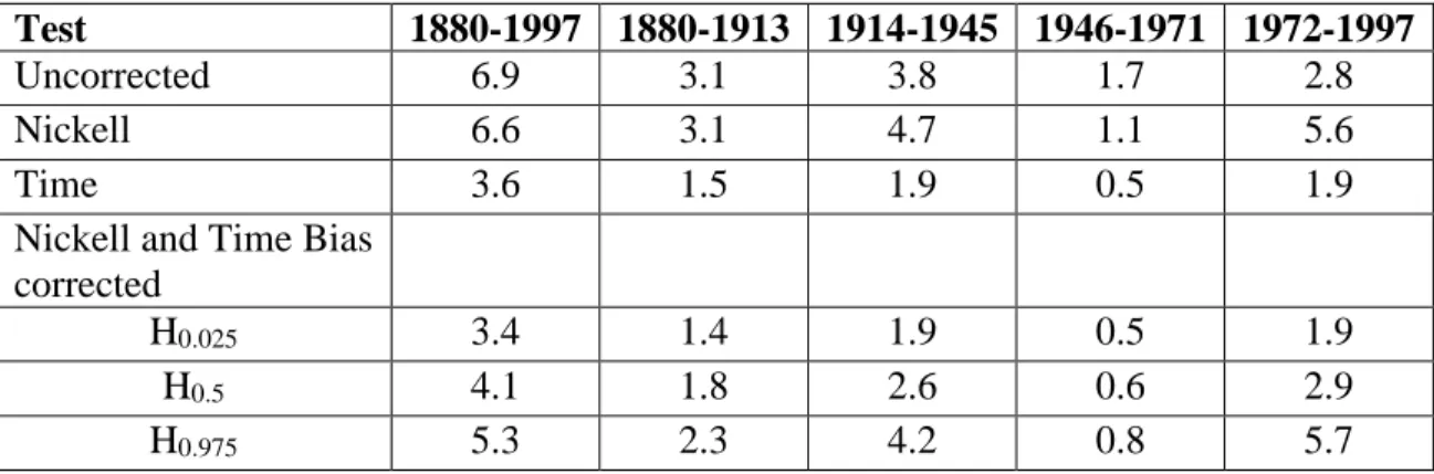
Although the Balassa-Samuelson effect tends to vary across regimes, the evidence suggests that it is present, and in the long-run the real exchange rate is not constant but conditioned on relative income levels. To explore the role of the Balassa-Samuelson effect in explaining the PPP puzzle, we examine both the conventional estimates of the half-life (based on the deviations from the mean) and the estimates controlling for the Balassa-Samuelson effect (based on the residuals in the real exchange rate regression). For the whole period, the (Nickel and time corrected) estimate of the half-life without the Balassa-Samuelson effect is between 3.4 and 5.3 years and is similar to conventional range of 3-5 years. Accounting for this effect lowers the estimated range to 1.9-2.6 years, which is much lower but still fairly long.13 The whole-period estimates, however, do not allow for a heterogeneous effect across regimes. Thus, we also estimate the half-life for each sub-period. The sub-period estimates (incorporating the Balassa-Samuelson effect) further reduce the half-life range to 0.4-0.7 years in the 1880-1913, 0.8-1.4 years in the 1914-1945, 0.3-0.6 years in the 1946-1971, and 0.7-1.2 years in the 1972-1997 sub-periods.14 These estimates suggest that the adjustment for a variable Balassa-Samuelson effect substantially lowers the persistence of the real exchange rate and helps resolve the PPP puzzle.
12 We also explore an extended real exchange rate relation that includes trade balance (a proxy
for net foreign assets) as an additional variable. The introduction of this variable makes little difference to the estimates of the Balassa-Samuelson effect (for the whole period as well as sub-periods).
13 The estimates for the whole period as well as for the sub-periods discussed below are based on
residuals in regressions with a time trend
14 Even the sub-period estimates without the Balassa-Samuelson effect imply shorter half-lives
since they partially account for the time variation in the real exchange rate by allowing a different mean for each regime. These estimates, however, do not reduce half-lives as much as the estimates with the Balassa-Samuelson effect.
8 Our paper is related to the Lothian and Taylor (2008) study, which uses data for three countries over a long span of time (nearly two centuries) to examine the importance of the Balassa-Samuelson effect. Their focus, however, is on testing the significance of this effect (assumed to be homogeneous over the entire period) within a framework that allows nonlinear reversion to the equilibrium real exchange rate and shifts in exchange rate volatility across regimes.15 The focus of our paper instead is on explaining the magnitudes and the signs of the Balassa-Samuelson effect under different regimes. Important contributions of our paper are to show that the estimates of the Balassa-Samuelson effect vary across regimes and to provide an explanation consistent with the modern versions of the Balassa-Samuelson model, which incorporate the terms of trade channel.
Our paper also relates to Chong, Jorda and Taylor (2012), who use panel data including a large number of countries and covering the recent period to provide support for the existence of a long-run Balassa-Samuelson relation. Their main objective is to measure adjustment to long-run equilibrium, which is purged of short-run frictions. Using a local projection approach, they find that the long-run adjustment has shorter half lives. Their results, however, do not explain the PPP puzzle related to short-run adjustment.16 Although explaining this puzzle is not the main concern of our paper, our empirical analysis does suggest that half lives of the short-run adjustment (after
15 Their estimate of the Balassa-Samuelson effectequals 0.125 for sterling-dollar and zero for the
sterling-franc real exchange rates. Interestingly, the average value of their estimates (0.0625) is not much different than our estimate of the average effect for the whole period without a time trend (0.068).
16 In fact, they restate the puzzle as “How can one reconcile the high-frequency variability and
flexibility of nominal exchange rates with the slow adjustment and persistence generated by frictions thought to have effects in the short term only?”
9 removing the long-run Balassa-Samuelson effect and allowing this effect to vary across periods) are not too long.
2. Data, Descriptive Evidence and Monetary Regimes
We have assembled annual data for 14 countries over the period 1880-1997 on real exchange rates relative to the U.S., real per capita GDP and the trade balance to GDP ratio. The countries covered, most of which are advanced countries are: Argentina, Australia, Canada, Denmark, Finland, France, Germany, Italy, Japan, Netherlands, Spain, Sweden, the UK and the US. For the data sources see the Data Appendix. Gaps in the annual data reflecting missing data during the World Wars for several countries were filled in by linear interpolation. The three series for each country ordered alphabetically are presented in figure 1 which shows both the actual data and the data filtered using a Hodrick-Prescott filter. The series presented are all relative to the U.S.
2.1 Monetary Regimes
Our data covers close to 12 decades. During that time span the world exhibited significant changes in the exchange rate regimes followed, as well as in the structure of the global economy, capital and trade flows. We demarcate the 12 decades into 4 distinct regimes: 1880-1913, the classical gold standard; l914-1945, the wars and interwar; 1946-1971, Bretton Woods; and 1972-1997 managed floating. These sub-periods represent not only different monetary regimes but (as discussed in Section 5) also diverse behavior of trade costs.
Our empirical analysis focuses on our basic sample, which ends in 1997 and does not cover the recent global recession. There has not been a major shift in either the monetary regime or the trade cost behavior since 1997. However, to explore whether the exclusion of the recent
10 period makes a difference to our results based on the basic sample, we also update our sample to 2014 and examine the sensitivity of the results to this extension.17
1880-1913
This was the period of the classical gold standard in which most countries of the world had fixed gold parities (in our sample Italy adhered to gold for only part of the period as did Argentina, Spain never did). It was also a period characterized by relatively low tariffs and non-tariff barriers in most countries (with the principal exception of the US), open capital markets, relatively flexible wages and prices and limited government intervention in the economy.
In this period most countries had relatively stable real exchange rates reflecting the fixed parity and relatively stable price levels. It was also a period of sustained growth across the world although with the principal exception of Canada and Sweden, not growing as rapidly as the US (see figure 1). In this period, there were massive capital flows from the advanced countries of Western Europe to the emerging countries of the day: Argentina, Australia and Canada. This was reflected in persistent current account surpluses in the former countries and deficits in the latter (Bordo, Eichengreen and Kim 1998).
1914-1945
This turbulent period marked a significant change in the policy regime and in structure. Most countries abandoned the gold standard during and after World War I and allowed their exchange rates to float, or they imposed extensive exchange and capital controls (Obstfeld and
17 The data in our basic sample has been carefully constructed to have consistent series across
different monetary regimes. For the update, we had to link series for recent data (from new sources) to the series in the basic sample (see Data Appendix).
11 Taylor 1998). The gold standard was reinstated from 1925-1936 as a Gold-exchange standard. It was followed by a period of heavily managed floating.
The 1930s were characterized by large increases in tariff and non-tariff barriers and extensive capital controls. The 1930s also was a period with considerable nominal rigidity and in which government intervention in the economy increased dramatically to protect income and employment from the shocks of the Great depression. World War II continued the trends of the 1930s.
In this period the real exchange rate was highly unstable with no distinct trend. Per capita real growth, although high in the 1920s, declined dramatically in most countries during the 1930s until they cut the link with gold (Eichengreen l992). There is little pattern of convergence with the US in the 1930s and substantial divergence in the war years (figure 1). The relationship between trade balances and the real exchange rate also appears to be weak in this period reflecting the disruption in trade and capital flows.
1946-1971
The Bretton Woods system established in 1944 required members to declare fixed
parities in terms of the dollar. It also required current account convertibility. The postwar era was characterized by significant declines in tariff barriers, continued restrictions on capital mobility, considerable government intervention in the macro economy and remarkable macro stability (Bordo 1993). Real exchange rates were stable. Economic growth in most countries was dramatic as they recovered from the war. The convergence that occurred in real per capita growth relative to the US is evident in figure 1.
12 1972-1997
In this period, the Bretton Woods system collapsed and was replaced by generalized managed floating. For the first 10-15 years real exchange rate volatility was relatively high, with a positive trend in most countries. During this period trade protection continued to decline and trade mushroomed. Also, restrictions on capital movements were gradually eliminated. After 1985 exchange rate volatility declined. The pattern of convergence in real per capita GDP with the US seems to emerge in figure 1 together with a positive (appreciating) trend in the real exchange rate until the 1990s. Finally, graphical analysis for this period seems also to suggest a negative relationship between the relative trade balance and the real exchange rate for a number of countries, especially Canada, Sweden and the UK.18
Figure 1 does not provide clear-cut evidence of a positive association between the real exchange rate and real per capita GDP relative to the U.S. across all countries and periods.19 Our
econometric analysis in Section 4 further examines the evidence by using techniques to extract the long-run relation and allowing the relation to shift across sub-periods. As the series for individual countries are not sufficiently long (to estimate the long-run relation) for different sub-periods, we use panel data methods to properly evaluate the evidence on the relationship between the real exchange rate and real income.
18 As a sensitivity exercise in Section 4.2 below we extend the study to include the period 1997
to 2014. A number of important institutional changes occurred which could significantly affect our empirical results. These include: the creation of the World Trade Organization ( WTO) in 1995; the establishment of the European Monetary Union in 1999; China’s membership in WTO in 2001; and the Financial Crisis and Great Recession 2007-2008 which led to the collapse of world trade for a year and a levelling off ever since. Surprisingly our empirical results basically hold up to the change in the environment.
19 Correlation coefficients between these variables show considerable variation across different
13
3. Theoretical Framework
This section develops a theoretical framework to compare different models of the long-run behavior of the real exchange rate and motivate the empirical relations estimated in the next section. We first discuss a basic model based on the conventional Balassa-Samuelson theory. We then consider two variants of the basic model, which introduce specialization in production and monopolistic competition. We use a simple setup with two countries (home and foreign), one factor (labor), and two categories of goods (traded and nontraded goods). In the basic model, all traded goods can be produced in both countries. The first variant assumes that each country is specialized in the production of a subset of traded goods and thus home and foreign goods are not perfect substitutes. Productivity changes in this model lead to an adjustment in the terms of trade as well as the relative price of nontraded goods. The second variant assumes monopolistic competition (with each country producing different varieties of a differentiated traded good), and introduces an additional adjustment mechanism through endogenous entry and exit of firms. As the key results of both variants are similar, we discuss the simpler first variant below, and make the second variant available as an appendix.
3.1 Basic Model
We focus on the equations of the model for the home economy. Symmetric equations are assumed for the foreign economy with an asterisk used to denote foreign variables and
parameters. As the paper is concerned only with the long-run effects, we ignore dynamics arising from nominal rigidities or international borrowing or lending, and simplify the analysis by using a static model. The aggregate consumption index is defined by the Cob-Douglas function:
1 1 (1 ) N T C C C
14 goods, and
is the share of nontraded goods in expenditure. To facilitate comparisons between the basic model and its variants, we can assume that there is a continuum of goods (or varieties) in nontraded and traded goods sectors.20Let
A
N andA
Tdenote labor productivities for nontraded and traded goods, which are assumed to be the same for all goods in each sector. Also, let qdenote the real exchange rate defined as the real value of home currency (i.e., the relative price of C in terms of *C ). Using a first-order log-linear approximation of model relations, we can derive a general form of the conventional Balassa-Samuelson relation for the real exchange rate as
* * *
ˆ ˆ ˆ ˆ
ˆ ( T N) ( T N)
q
A A
A A , (1)where a hat over a variable denotes the log deviation of the variable from its initial value.21
Empirical analysis often uses a simple form of this relation, where the real exchange depends on the home-foreign differential in traded goods productivity or income per capita. This form can be derived by making the following two assumptions:
Assumption 1.
*. Assumption 2.AˆN Aˆ*N.The first assumption abstracts from international differences in tastes (i.e., the share parameters in the aggregate consumption index). The second assumption accords with the view often
20 To derive the standard Balassa-Samuelson relation for this case, however, we also need to
assume zero trade costs so that all traded goods (varieties) are produced in both countries and the law of one price holds for each good.
21 Derivation of this relation under the assumption of a continuum of nontraded and traded goods
15 associated with the Balassa-Samuelson theory that nontraded goods generally represent services, which are produced by similar technology across countries. Under assumptions 1 and 2, relation (1) simplifies to: qˆ
(AˆT Aˆ*T). Thus in the simple version, the home-foreign differential in the traded goods productivity is the only determinant of the real exchange rate and the coefficient of the productivity differential equals the share of nontraded goods.The simple version also implies a relation that links the real exchange rate to the differential between real income per capita in the home and foreign country. Let denote real income per capita and assume that it is proportional to real income per worker. Assuming that trade is balanced and noting that real income (equal to real output) per worker simply equals the real wage (since labor is the only factor and there are zero profits), we can obtain (see the online appendix)
ˆ ˆ
ˆ N (1 ) T
y
A
A . (2)Next, use (2) and its foreign counterpart to substitute for and in (1) and get:
* * * * * * ˆ ˆ ˆ ˆ (ˆ ˆ ) ( ) (ˆ ) 1 1 N N (1 )(1 ) N q y y A A y A
. Under assumptions 1 and 2, this
relation reduces to * ˆ (ˆ ˆ ) (1 ) q
y y
. (3)The coefficient of income differential in (3) - the Balassa-Samuelson effect- is larger than the share of the nontraded goods. The magnitude of this coefficient, however, is sensitive to the assumption about the productivity differential for nontraded goods. For example, consider a modified version, which replaces assumption 2 by the following assumption:
y
ˆ
T16 Assumption 3. AˆN Aˆ*N
(AˆT AˆT*), 0
1.Assumption 3 allows the nontraded good productivity differential to vary, but for simplicity, assumes a proportional relation between the productivity differentials for nontraded and traded goods. To capture the view that international productivity differences are less important for nontraded than traded goods, the elasticity of the nontraded good productivity differential with respect to the traded good differential (λ) is assumed to be less than one. Using assumptions 1 and 3 along with (1), (2) and its foreign counterpart, we modify (3) as
* (1 ) ˆ (ˆ ˆ ) 1 q
y y
. (4)The alternative assumption 3 still allows the real exchange rate to be expressed as a function of the income differential, but this differential’s coefficient is smaller than under assumption 2.
3.2 Specialization in Production
This section examines how the results change if the basic model is modified to let the home and foreign countries be specialized in the production of traded goods22. In this and the monopolistic competition variants, productivity changes affect the real exchange rate not only directly but also indirectly via the terms of trade channel. The indirect effect and the degree to which the indirect effect offsets the direct effect have been explored quantitatively as well as analytically (e.g., Corsetti, Dedola and Leduc, 2008; Choudhri and Schembri, 2010). The relationship of the real exchange rate to the income differential, however, has not been
examined. A contribution of this section is to derive a relation expressing the real exchange rate
22 This variation can be motivated by the assumption that each country has a comparative
17 as a function of the income differential. We are also able to show that the exchange rate relation derived for the specialization model also holds for the monopolistic competition model.
Define the consumption index for traded goods as
/( 1) ( 1)/ ( 1)/ ( ) ( ) T H H F F C C C , (5) where /( 1) ( 1)/ ( ) H H H j C C j dj
and * /( 1) * ( 1)/ * ( ) F F F j C C j dj
representdomestic consumption indexes for home (exported) goods subset
H and foreign (imported) goods subset
F ;
H and
F are preference parameters for home and foreign goods and
isthe elasticity of substitution between these goods; and
is the elasticity of substitution between varieties of each subset. The above specification allows for home bias in preferences as well as for asymmetric elasticities of substitution between and within home and foreign bundles.We also introduce trade costs in this model and assume that they take the form of iceberg costs such that ( 1) units of a product need to be exported to deliver 1 unit in the importing
country. The price indexes for
C C
T,
HandC
F are given by1/(1 ) 1 1 H F T H F p p p
, (6) where * 1/(1 ) 1/(1 ) 1 * 1 * ( ) , { ( )} H F H j H F j F p p j dj p p j dj
;p
H( )
j
is the homereal price (in terms of C) of home good j,
p
F( )
j
* is the foreign real price (also in terms of C) of18 individual goods in terms of C are connected by the real exchange rate to those in terms of C* as
* * * *
( )
( ),
( )
( )
H H F F
qp
j
p
j
qp
j
p
j
. (7)Letting
z
p
H/ (
p
F)
denote the terms of trade for the home country and normalizing1
H F
p
p
in the initial state, we can modify the relation for the real exchange rate under incomplete specialization as * * * * * * ˆ ˆ ˆ ˆ ˆ ( H N) ( F N) (1 ) ˆ q A A A A z, (8) whereA
H and * FA
represent labor productivities in the production of home and foreign tradedgoods,
(
H)
1
1 (
F/ )
1 is the initial share of home goods in the home traded goodbasket while
*
(
*H/ )
1
1 (
F*)
1 is the share of home goods in the foreign basket.23 Note that increases and *decreases as trade cost index,
, increases. Also, note that * in the presence of trade costs even if there is no home bias in preferences(
H
H*)
. The real exchange rate relation (8) now includes a terms of trade effect (represented by the third term), thorough which productivity differentials can potentially offset the standard Balassa-Samuelson effects (captured by the first two terms), as discussed below. Real income per worker also depends on the terms of trade and the income relation is modified asˆ ˆ
ˆ N (1 ) H (1 )(1 )ˆ
y
A
A
z. (9)
19 Letting
* denote the home goods share differential (between the domestic and foreign traded goods bundles) and using assumptions 1 and 2, the solution for the terms of trade can be derived as24 * ˆ ˆ ( ) ˆ (1 ) H F A A z . (10)Note that if / (1), then (1) 0, and we have the typical result that an improvement in home productivity (relative to foreign productivity) will worsen the terms of trade.25
To relate the real exchange rate to the income differential, we first substitute the value of zˆ from (10) into (8), (9) and its corresponding foreign equation, use assumptions 1 and 2 (as in the basic model), and obtain
* (1 ) 1 / ˆ ˆ ˆ ( ) (1 ) H F q A A , (11) * (1 ) 1 ˆ ˆ* ˆ ˆ (1 ) ( ) (1 ) H F y y A A . (12)
We then use (11) and (12) to get
* ˆ (ˆ ˆ ) (1 ) q
y y
, (13)24 As shown in the online appendix, the effect of ˆ
N
A on the trade balance is completely offset by that of AˆN* under assumptions 1 and 2, and thus the terms of trade are not affected by labor productivities for nontraded goods.
25 If
/ (1 )
, then we obtain the case highlighted in Corsetti, Dedola and Leduc (2008), where higher home productivity, in fact, improves the terms of trade and thus enhances the Balassa-Samuelson effect.
20 where 1 / (1 ) 1
. As (13) indicates, the Balassa-Samuelson effect in the specialization
model is different than in the conventional model [relation (3)]. In the (typically-assumed) case of / (1),
is less than one and decreases as increases or
decreases. In this case, moreover,
is negative if / (1)/ (1). Thus, incorporating the terms of trade effect not only decreases the Balassa-Samuelson effect [compare (13) with (3)], but also reverses the sign of the effect if the substitution elasticity is sufficiently low or the home good differential is sufficiently high.In the online appendix, we discuss the monopolistic competition version of the model, and show that this variant also yields relation (13). Under monopolistic competition, endogenous entry/exit (adjustment on the extensive margin) magnifies the effect of the traded- goods
productivity differential on both the real exchange rate and the income differential. Remarkably, however, the degree of magnification is the same for both variables, and the relation between qˆ
and
y y
ˆ ˆ
*is not altered.3.3 Empirical Implementation
Our long-run theoretical relation linking the real exchange rate to the income differential is based on a two-country model. One way to empirically implement it to a multi-country world is to let the home country represent an individual country and consider the foreign country an aggregate of the country’s trading partners. Assuming that the coefficients (except the constant term) are homogeneous across countries, the long-run empirical relation for panel data can be specified as
21
, 0 1 , , ,
ln
q
cw t
c
(ln
y
c t
ln
y
wc t)
e
c t, (14)where for period t,
q
cw t, is the trade share weighted average of bilateral real exchange rates (theeffective real exchange rate) for country c,
y
wc t, is the similarly weighted average of per-capitaincomes of county c’s trading partners, and
e
c t, is the error term. In the simple version of theconventional Balassa-Samuelson model (relation (3) based on assumptions 1 and 2),
1 equals / (1 ) . The value of this coefficient would be smaller in the modified version, which allows the nontraded good productivity differential to vary (relation (4) based on assumptions 1 and 3). In this case,
1 equals (1 ) / (1 )with 1. In the modern version of theBalassa-Samuelson model, which incorporates specialized production or monopolistic competition [relation (13)],
1 equals / (1) where 1 ( / ) / ( (1 )) is less than 1, and can even be negative under sufficiently low
or high .To estimate (14), we require data on bilateral real exchange rates and trade shares as well as per-capita incomes for all economies to measure
q
cw t, andy
wc t, . As our historical data set includes data only for a subset of countries and lacks data on bilateral trade shares for the full sample, we resort to estimating a bilateral version of (14). The bilateral version does not fully account for the general equilibrium effects and we briefly explore the potential bias arising from this limitation.Choose the United States as the reference country, use subscript u to denote US variables, and define the country ’s bilateral real exchange rate with the US as
q
cu t, (the real value of thecurrency of country c in terms of US dollar). Letting
q
%
cw t, denote c’s effective real exchange rate c22 based on US weights, we have
q
cu t,
q
%
cw t,/
q
uw t, . Next, subtracting relation (14) for US from thatfor country c, and noting that
ln
q
cw t,
ln
q
uw t,
ln
q
cw t,
ln
q
cu t,
ln
q
%
cw t, , we obtain, 0 1 , , ,
ln
q
cu t
(ln
y
c t
ln
y
u t)
e
c t
, (15)where
0
0c
0u ande
c t,(
e
c t,
e
u t,)
1(ln
y
wu t,
ln
y
wc t,) (ln
q
%
cw t,
ln
q
cw t,)
. Thus the bilateral relation (15) includes the effect of differences in the weights for country c and the US on the indexes for world income and the effective real exchange rate (the last two terms in the expression fore
c t
,). The omission of these variables could introduce a bias in the estimation of1
, if they are correlated with the income differential term. However, there seems to be no reason to suspect a systematic association between trade share weights (primarily determined by location) and income levels.We estimate (15) in the next section. If assumption 1 does not hold,
1would differ across countries, and not accounting for these differences would introduce cross-sectional dependence between relations for different non-US countries and we introduce time effects in our panel estimates to account for this possibility. We also estimate the model with and without a time trend. The trend term could allow for the possible effect of changes in parameters such as trade costs and the share of nontraded goods, which are treated as constants in our model forsimplicity. This term could also capture the effect of deterministic trends in the productivity differential for nontraded goods if there are departures from assumptions 2 or 3.26 Finally, we
26 A deterministic trend could also be present in the traded goods productivity differential.
However, although the income differential and the real exchange rate series would have a deterministic trend in this case, the relation between these variables would not include the trend term.
23 also consider the possibility that the net foreign assets ratio does not converge to a unique value in steady state. In this case, trade balance (relative to income) would not be constant in the long run, and this variable would also be included in the real exchange rate relation. To allow for this possibility, we also estimated the bilateral version of the empirical model with the trade balance differential between country c and the US as an additional variable.27
4. Empirical Analysis
4.1 Stationarity tests and real exchange rate persistence
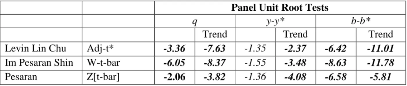
In Table 1 we present panel unit root tests for the full sample period. Three different tests are reported: the Adj-t* test of Levin, Lin and Chu (2002), the W-t-bar test of Im, Pesaran and
Shin (2003) and the Z[t-bar] test of Pesaran (2003). These tests always reject non-stationarity at the 5% or 1% level for the real exchange rate and the trade balance term. Productivity
differentials (measured by per capita income differentials) prove to be stationary at both the 1% and 5% levels on the basis of all three tests when a time trend is included. The panel unit root tests for our four different sub samples are presented in Table 2 and it is interesting to note that the rejection of nonstationarity is not as clear cut in the cases of the real exchange rate and trade balance differential as it was for the full sample period. In terms of the real exchange rate, there is more evidence in favor of stationarity for the two post World War II sub samples.
Table 3 reports the half-lives calculated for the real exchange rates using the method of Choi, Mark and Sul (2006). The full period results fall within the conventional 3 – 5 year range.
27 Letting c
b
denote the balance of trade of a country, the global exchange rate relation ismodified as
ln
q
cw t,
0c
1(ln
y
c t,
ln
y
wc t,)
2b
c t,
e
c t, , which implies the following bilateral relation:ln
q
cu t,
0
c
1(ln
y
c t,
ln
y
u t,)
2(
b
c t,
b
u t,)
e
c t
, .24 As would be expected, the two fixed rate periods – the Gold Standard and Bretton Woods – produce the fastest adjustment speeds, with Bretton Woods delivering the tightest range of 0.5 to 0.8. The two floating rate periods – inter war and post Bretton Woods - produce slower, although similar, adjustment speeds.
4.2 Group Mean and Panel Estimates
The long-run effect of the productivity differential on the real exchange rate is estimated by Group Mean (GM) and Panel DOLS (PDOLS) procedures. The group mean estimates are calculated by estimating N separate regressions and calculating the coefficient means. To account for cross-section dependence the series are cross sectionally demeaned before applying the estimator and the significance of the estimated coefficients is based on autocorrelations consistent standard errors. The PDOLS procedure provides a fully parametric estimator of the long run coefficients. In this context it involves a regression of the level of the real exchange rate on the levels of the explanatory variables and leads and lags of the differences of the explanatory variables. To account for cross-sectional dependence, time dummies are included in the PDOLS regressions and the PDOLS significance is based on Driscoll and Kray (1998) standard errors, which are heteroskedasticity consistent and robust to general forms of cross-sectional (spatial) and temporal dependence (see Hoeckle, 2007). The relevant specifications are reported in the notes of tables 4 and 5.
The GM and PDOLS procedures provide unbiased estimates of the coefficients in the long run relation if the variables in the relation are nonstationary or mixed stationary and non-stationary and cointegrated. As discussed above, the evidence for nonstationarity of the real exchange rate and productivity differential based on sub-samples is mixed. If these variables are
25 assumed to be nonstationary, the evidence on half lives of the residuals (discussed below)
suggests that they are cointegrated.
In tables 4 and 5 we present the estimates for our base line productivity specification for the full sample and the four sub-samples. Since we found evidence of cross-sectional dependence in our panel estimates (discussed further below), we only report estimates where cross-sectional dependence is accounted for by time dummies and demeaning the series.28 The results in the GM row are for the simple group mean and these give a statistically significant coefficient of 0.19 in the specification without a trend and 0.22 in the specification with a time trend. The PDOLS estimates are similar and significant both with and without a common trend, although the result of the latter test is significant only at 10% when an individual trend is used.
The results for the various sub-sample periods are reported in Table 5 and show considerable variation across regimes. In the Classical Gold standard period, 1880-1913, the coefficient values on the relative productivity term are all positive, significant and of a similar order of magnitude with and without a trend (irrespective of the trend being common or
individual). The values, in the range of 0.13 to 0.25 are clearly smaller than that expected in the traditional Balassa-Samuelson narrative but (as explained below) are consistent with the modern versions presented in Section 3. Moving into the period 1914-1945, we note that the sign flips from being positive to significantly negative in all cases and the magnitude of the coefficient using the Panel DOLS estimators is approximately double the size of the coefficient in the case of the GM estimator.
28 As discussed in Section 3.4, departures from assumption 1 (symmetric shares) could lead to
26 In the Bretton Woods period the results differ both with respect to whether a trend is included or not and also depending on the estimator used. For example the GM results produce an insignificantly negative outcome in the no trend case and a significantly negative outcome in the trend case. With the Panel DOLS estimator the results all produce a small but insignificantly positive coefficient on the relative productivity term. In the post Bretton Woods period the results show a clear positive and statistically significant coefficient with the coefficient varying from 0.20 to 1.18 depending on the specification. An interesting aspect of the post Bretton Woods results is that the coefficient on the relative income term falls from 1.18 to 0.58 when an individual trend is used rather than a common trend.
We have performed two set of robustness exercises. First, we have re-estimated the Balassa-Samuelson effects after introducing the trade balance as an additional regressor and the results are not qualitatively affected. In the second set, we have explored alternative estimators based on an error-correction specification. Specifically, we have used Mean Group (Pesaran and Smith, 1995) and Pooled Mean Group (Pesaran, Shin and Smith, 2004) estimators which
consider the case when all variables are I(1) and cointegrated. These estimators are indicated in the case of nonstationary heterogeneous panels, especially if the number of groups or time periods is large. In order to control for potential cross-sectional dependence, the series are first demeaned. Again, overall these results seem to confirm, in terms of sign, size and significance those obtained using the PDOLS and GM estimators, especially if individual trends are included. Both robustness exercises are omitted for brevity, but are available upon request.
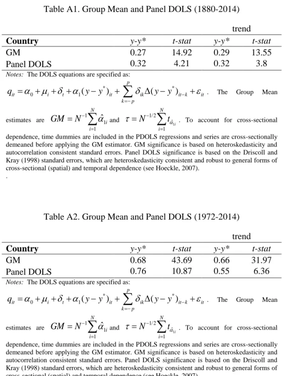
We also explored the robustness of our results to extending our sample to 2014. The results for our baseline specification for 1972-2014 and 1880-2014 are shown in the Appendix, Tables A1 and A2. Extending the last sub-sample to 2014 does not make much difference to the
27 key result that the income coefficient for the post Bretton Woods period remains significantly positive and much larger than for the previous sub-periods. However, extending the sample makes the coefficient less sensitive to the introduction of individual trends and reduces its magnitude in most cases. Finally, note that the income coefficient for 1880-2014 is larger than for 1880-1997 as extending the full sample gives more weight to the last regime which has stronger Balassa-Samuelson effects. Again, an interesting and puzzling result of the empirical analysis is the evidence of changes in the sign and the magnitude of the coefficient across sub samples. An explanation of these results in terms of the modern version of the
Balassa-Samuelson theory is suggested in section 5.
4.3 Half Lives of Residuals
The half-life estimates discussed above do not account for the influence of the productivity differential. To control for this effect, Table 6 shows estimates of half-lives of residuals obtained from relations that contain the productivity variable. We consider two
specifications based on panel DOLS: the first excludes the first difference terms (no fd’s) and the second includes these terms (fd’s). The first specification controls only for the long-run effect of the productivity differential while the second specification also controls for the short-run effects of the differential captured by the first difference terms. For each specification, half-life
estimates are presented for relations with and without a time trend. As already noted above, even without the productivity effect half-lives tend to be shorter for sub samples than for the whole sample. Controlling for this effect, sub sample half-lives are significantly reduced, especially if short term effects are also incorporated. The half-lives are further reduced when a time trend is included, thereby perhaps suggesting that our productivity term may not capture the totality of productivity trends. The statistical significance of these results indicates clear evidence of
28 cointegration in the panel DOLS estimates. It is interesting to note that it is possible to provide a resolution for the PPP puzzle in the context of a linear model by controlling for productivity effects and allowing a time trend. For example, the half-life range of the real exchange rate in Table 2 (without controls) is from 1.9 to 5.7 years for the post Bretton Woods period. In the presence of a time trend, the half-life range in Table 6 reduces sharply to 0.8-1.4 years after controlling for the long-run productivity effect and 0.7-1.2 years after also controlling for the short-run effect. The interwar period also has a long half-life range, and controls also
significantly shorten this range.
Half lives are somewhat larger for the full as well as the last sub-sample if the data set is updated to 2014. However, we still find that the half lives decrease sharply if they are estimated after controlling for the factors suggested by the linear Balassa-Samuelson Model (the detailed results are available on request).
5. Explaining the Results
In this section, we examine if the Balassa-Samuelson theory is capable of explaining the results discussed above. We consider both the conventional and the modern versions of the theory.
5.1 The Conventional Version
The estimates of the income coefficient in the PDOLS and GM regressions are difficult to reconcile with the conventional Balassa-Samuelson model. The share of nontraded goods (
) is typically assumed to be greater than 0.5. For 0.5, the productivity effect in (3) predicted by the conventional model (simplified by assumptions 1 and 2) would equal or exceed 1.0. Our29 estimates of the coefficient of the productivity differential for the full sample range from 0.13 to 0.22 and are much below the predicted value.
Small values of the productivity coefficient could be potentially explained by the modification of the model that allows the productivity differential for nontraded goods to vary (as in relation (4) based on assumption 3 instead of assumption 2). However, (the elasticity of the nontraded traded good productivity differential with respect to the traded good differential) would have to be fairly large to account for the low estimates of the productivity coefficient. For example, to explain the full-sample range for the productivity coefficient, we would need values, of between 0.64 and 0.77 for 0.5, and between 0.70 and 0.81 for 0.6. Such high
values of seem implausible as they imply that international differences in nontraded goods productivity growth tend to be substantial relative to the productivity growth differences for traded goods.
Estimates of the coefficients for the subsamples show considerable variation across periods and are even harder to explain by the conventional Balassa-Samuelson model. Estimated values are positive but small (below 0.25) in the gold standard period; are negative (between -0.17 and -0.42) in the interwar period; have an ambiguous sign (range from -0.33 to 0.12) in the Bretton-Woods period; and are positive, and on average, larger (within a wide range from 0.2 to 1.18) in the post Bretton-Woods period. The conventional model or its modification do not suggest an explanation of why the productivity coefficient would be negative in some periods and why it would differ so much from one period to another.
30
5.2 Modern Versions
We next examine whether the modern version of the Balassa-Samuelson model based on specialization in production or monopolistic competition can explain the range of estimates of the productivity effect. For both versions, the productivity effect is given by (13) and depends not only on
, but also on
(the elasticity of substitution between home and foreign tradables) and (the home goods share differential). Shifts in these parameters could potentially account for the cross-period variation in the productivity coefficient. An important reason for such shifts is the behavior of trade costs, which changed dramatically across the four sub-periods.29 Trade costs fell prior to World War I mainly as a result of reduction in transport costs andimprovements in information technology. They rose sharply in the interwar period largely due to the escalation of tariff and nontariff barriers caused by the Great Depression. The behavior of trade costs was mixed in the Bretton Woods period as some trade restrictions were relaxed after World War II, but other restrictions were introduced by many countries to deal with trade deficits under fixed exchange rates. Trade costs fell in the post Bretton Woods period because of
significant reductions in trade barriers resulting from regional and international trade agreements and in transportation costs due to technological improvements.
Since
*, changes in trade costs would shift via their effect on and *. An increase in trade costs would raise the prices of imports and exports, and for 1 , would increase and decrease *and hence increase .30 Thus we would expect to increase in the
29 Jacks, Meissner and Novy (2009) assign an important role to trade costs in explaining the twin
booms in international trade before World War I and after World War II as well as the international trade bust in the interwar period.
30 Trade costs could also affect the share of nontraded good if there are departures from the
31 interwar period and decrease after the Bretton Woods period. Higher trade costs, especially larger nontariff barriers, could also reduce the range of foreign goods available in the home market as well as the range of home good available abroad. Such changes could make imported and exported goods less substitutable with local goods, and decrease
. Thus
could also have changed across the four regimes in a direction opposite to that of .It is interesting to explore whether realistic values of
, and
for the four regimes could explain the magnitude and the signs of the productivity coefficient in each regime. There is much interest in estimating
(often referred to as the “Armington elasticity”), which plays an important role in a wide variety of macroeconomic and international trade models.Macroeconomic models typically calibrate or estimate its value at the aggregate level to be between 0.5 and 2.0.31 Studies using disaggregated international trade data suggest much larger estimates of the elasticity, but these estimates are based on a specification (different from ours) which assumes that the elasticity between a pair of varieties is the same regardless of where they are produced.32 In an alternative specification that allows the Armington elasticity to differ from the elasticity between foreign varieties, Feenstra, Luck, Obstfeld, and Russ (2014) find that estimates based on disaggregated US data indicate that the Armington elasticity is less than the between-varieties elasticity in half the cases and is not inconsistent with the range from 1.0 to 2.0 often assumed in the macroeconomic models. In the simple case of symmetric import shares in
one (i.e., aggregate consumption index is a Cobb-Douglas function of traded and nontraded bundles of goods). In this case, changes in trade costs would affect
via their effect on the price of traded goods. If this elasticity is less than unity, higher trade costs would decrease
in the interwar period while lower trade costs would increase it in the post Bretton Woods period.31 Estimation of macroeconomic models typically yields an estimate of the elasticity close to the
lower half of this range (e.g., see Bergin, 2004, Lubik and Schorfheide, 2005).
32 See, for example, Imbs and Mejean (2011) for estimates of the elasticity, allowing it to be
32 tradable bundles
(1
*)
, the home goods share differential can be expressed as 21. Estimates of
and 1 can be derived from sectoral production and trade data.33 For OECD countries, such data are available since 1970, and estimates based on this data suggest values of
above 0.6 and of below 0.80 (implying below 0.6).34The role of
and in determining the productivity coefficient in the model with specialization or monopolistic competition is illustrated in Figure 2. For 0.65, the figureshows the relation between the productivity coefficient and
for two values of , a low value of 0.4 and a high value of 0.8. We let
vary between 1.0 and 2.0. The productivity coefficient is an increasing function of
, and a higher shifts the function down (for 1).Interestingly, the ranges for
and shown in the figure are capable of accounting for not only large negative values of the productivity coefficient estimated for the interwar period, but also large positive values generally estimated for the post Bretton Woods period. For between 0.4 and 0.8, values of
in the 1.2-1.4 range could generate low positive values of the productivity coefficient consistent with the gold standard period (as well as the whole period). As can be seen from the figure, however, an increase in alone would not explain the sharp drop in theestimate of the productivity coefficient for the interwar period. A small decrease in
would also be needed to account for this result. A combination of an increase in
and a decrease in could bring about the estimated changes in the productivity coefficient between the Bretton33 The estimates of
are sensitive to how traded goods are classified. A narrow measureidentifies traded goods with Manufacturing, Agriculture and Mining sectors. A broader measure would also include portions of Elecricity and Gas, Transportation and Communication, and Financial Services sectors that have significant trade.
34 See, for example, Choudhri and Marasco (2013), who estimate average values of
1 and 1 for a set of OECD countries to equal 0.36 and 0.22, respectively.
33 Woods and the interwar periods. Further changes in this direction could produce the results for the post Bretton Woods period.
Our explanation of inter-regime variation of income coefficient is based on shifts in parameters, especiallyand
, which are difficult to estimate and direct empirical evidence is not available on how these parameters may have shifted over time in our sample. However, is a function of trade costs and changes in these costs across different sub-periods provide indirect evidence on whether implied shifts in fit our explanation. Jacks et al. (2008) use a structural gravity model based on Anderson and van Wincoop (2003) to estimate bilateral trade costs of the USA, UK and France with their trading partners from 1870 to 2000.35 Although their focus is on intra-period changes in average trade costs of these countries for pre-War I, interwar and post-War II periods, we use their estimates to examine inter-period changes for our four sub-periods.36 To highlight these changes, Table 7 shows the three countries’ average trade cost for each sub-period.37 As the estimation methodology is more suitable for measuring changes than levels of trade costs, trade costs in the gold standard period are normalized to 100.38
35 The estimation procedure requires bilateral trade data (including internal flows) and estimates
of the elasticity of substitution based on a one-tier utility function (with the elasticity of substitution between home and foreign goods equal to the between-varieties elasticity).
36 Average trade cost of each country represents an average of its bilateral trade costs across its
trading partners. Trade costs are expressed in terms of tariff equivalents defined as the iceberg trade cost index minus one.
37 The annual trade cost of each country was calculated as the trade share weighted average of its
bilateral costs. The sub-period average represents the mean value of annual trade costs.
38 Internal trade costs are normalized to zero to estimate international trade costs. Levels of
international trade costs but not changes in these costs are sensitive to this normalization. Estimates of trade costs, moreover, are a function of the substitution elasticity. Trade cost levels are more sensitive than changes to variations in the value of the substitution elasticity.