A Dynamic and Reliability-Driven Scheduling Algorithm for Parallel
Real-time Jobs on Heterogeneous Clusters
Xiao Qin
Department of Computer Science,
New Mexico Institute of Mining and Technology, 801 Leroy Place, Socorro, New Mexico 87801-4796
Hong Jiang
Department of Computer Science and Engineering University of Nebraska-Lincoln
Lincoln, NE 68588-0115 [email protected] Proposed running head:
DYNAMIC RELIABILITY DRIVEN REAL-TIME SCHEDULING ON CLUSTERS
Address for Manuscript correspondence:
Xiao Qin
Department of Computer Science,
New Mexico Institute of Mining and Technology, 801 Leroy Place, Socorro, New Mexico 87801-4796 E-mail: [email protected]
Abstract
In this paper, a heuristic dynamic scheduling scheme for parallel real-time jobs executing on a heterogeneous cluster is presented. In our system model, parallel real-time jobs, which are modeled by directed acyclic graphs, arrive at a heterogeneous cluster following a Poisson process. A job is said to be feasible if all its tasks meet their respective deadlines. The scheduling algorithm proposed in this paper takes reliability measures into account, thereby enhancing the reliability of heterogeneous clusters without any additional hardware cost. To make scheduling results more realistic and precise, we incorporate scheduling and dispatching times into the proposed scheduling approach. An admission control mechanism is in place so that parallel real-time jobs whose deadlines cannot be guaranteed are rejected by the system. For experimental performance study, we have considered a real world application as well as synthetic workloads. Simulation results show that compared with existing scheduling algorithms in the literature, our scheduling algorithm reduces reliability cost by up to 71.4% (with an average of 63.7%) while improving schedulability over a spectrum of workload and system parameters. Furthermore, results suggest that shortening scheduling times leads to a higher guarantee ratio. Hence, if parallel scheduling algorithms are applied to shorten scheduling times, the performance of heterogeneous clusters will be further enhanced.
Keywords: Dynamic scheduling, real-time, parallel processing, heterogeneous clusters, cluster computing, reliability cost, performance evaluation.
1. Introduction
Heterogeneous clusters have become widely used for scientific and commercial applications. These systems require a mixture of general-purpose machines, programmable digital machines, and application specific integrated circuits [33]. A heterogeneous cluster involves multiple heterogeneous modules that interact with one another to solve a problem [34][41]. In a heterogeneous cluster, applications comprise multiple subtasks that have diverse execution requirements. The subtasks must be assigned to machines and ordered for execution in such a way that the overall application execution time is minimized [18].
Recently, heterogeneous clusters have also been employed in real-time applications [43], in which the systems depend not only on results of computation, but also on time instants at which these results become available. The consequences of missing deadlines of hard real-time systems may be catastrophic, whereas such consequences for soft real-time systems are relatively less damaging.
Examples of hard real-time applications include aircraft control, radar for tracking missiles, and medical electronics. On-line transaction processing systems are examples of soft real-time applications. In real-time applications, reliability is one of the most important issues. Due to the critical nature of jobs executed in many real-time systems, high reliability becomes an inherent requirement of such systems, and this is especially true for hard real-time applications.
Growing evidence shows that scheduling is a key factor in obtaining high reliability and performance in heterogeneous clusters supporting real-time applications. The objective of real-time scheduling is to map tasks onto machines and order their execution so that task precedence requirements are satisfied and a minimum schedule length, when attainable, is given. Besides achieving this conventional objective, the dynamic scheduling strategy proposed in this paper provides high reliability for non-preemptive, aperiodic, real-time jobs without any additional hardware cost. In particular, we have developed a framework of real-time scheduling by which parallel jobs are scheduled dynamically, as they arrive at a heterogeneous cluster. In this framework, a designated machine, called scheduler, is responsible for dynamically scheduling real-time jobs as they arrive, and dispatching them to other machines, called processing elements, to execute. The proposed algorithm takes into account dispatching and scheduling times in addition to reliability costs, and these factors have been neglected by most scheduling schemes that deal with real-time heterogeneous clusters. This approach is shown by our simulation studies to not only make real-time jobs more predictable and reliable, but also make the scheduling more realistic.
The paper is organized as follows. In Section 2, work reported in the literature that is the most relevant to our work is briefly described. The system and reliability models are presented in Section 3. Section 4 proposes a novel dynamic scheduling algorithm. Performance evaluation is presented in Section 5. Finally, Section 6 concludes the paper by summarizing the main contributions of this paper and commenting on future directions of this work.
2. Related Work
Many scheduling algorithms have been proposed in the literature to support real-time systems. Real-time scheduling algorithms are classified into two categories: static (off-line) [1][15][21][24] [27][29][32] and dynamic (on-line) [13][17][19][22][31][36]. Very recently, Palis addressed task-scheduling problems in the context of reservation-based real-time systems that provide quality of service guarantees [22]. Real-time tasks in Palis’s scheduling framework are preemptive [22],
whereas it is assumed in our scheduling model that real-time tasks are non-preemptive. Moreover, the algorithm proposed by Palis [22] as well as many other algorithms presented in [21][36] were designed for independent real-time tasks. In contrast, our proposed algorithm, like those described in [15][24][27][29], can schedule tasks with precedence constraints, which are represented by directed acyclic graphs (DAG). We recently extended non-time DAGs into time DAGs to study real-time scheduling of tasks with precedence constraints [24]. However, these algorithms, while considering precedence constraints, belong to the static category, limiting their applications to offline scheduling only. Furthermore, most of these real-time scheduling algorithms are designed for homogeneous systems, making them unsuitable for heterogeneous systems.
In the literature, parallel jobs have often been represented by DAGs [4][7][15][29][41]. Wu et al. proposed a runtime parallel incremental DAG scheduling approach [41]. Cosnard et al. developed a scheduling algorithm for a parameterized DAG, which first derives symbolic linear clusters and then assigns task clusters to machines [7]. As for distributed computing, a typical model is the fork-join paradigm [30], where main program thread runs on one processor and spawns a number of tasks from time-to-time. Sahni and Vairaktarakis addressed the scheduling problem in the fork-join paradigm, and developed efficient heuristics to obtain minimum finish time schedules for single-master processor and multiple-master systems [30]. The scheduling algorithms in these three studies, however, were also designed for homogeneous systems.
The studies in heterogeneous clusters reveal a number of challenges, which include load balancing [3][42][25], resource management [10] and scheduling [5][6][38]. The issue of scheduling on heterogeneous systems has been addressed in many papers [3][6][8][11][28][29][35][37]. It is suggested that minimizing a task's completion time leads to a minimal start time of the task [18][37]. Topcuoglu et al. studied two efficient and low-complexity heuristics for DAGs: the heterogeneous Earliest-Finish-Time (HEFT) algorithm and the Critical-Path-on-a-Machine (CPOP) algorithm [37]. Iverson and Özgüner proposed a matching and scheduling framework where multiple applications compete for computational resources on networks [11]. Maheswaran and Siegel investigated a dynamic matching and scheduling algorithm for heterogeneous system [18], whereas Beaumont proposed a static scheduling algorithm that based on a realistic model for heterogeneous networks of workstations. To consider reliability of different resources in a system while making scheduling decisions, Doğan and Özgüner introduced two cost functions that were incorporated into a matching and scheduling algorithm for tasks with precedence constraints [8]. As computational Grids have
emerged as new platforms for high-performance computing, grids have become a new frontier for research in the area of scheduling and resource management. Arora, Das, and Biswas proposed a new scheduling algorithm for a generalized heterogeneous Grid environment [3]. Unfortunately, all these scheduling algorithms assumed that tasks are non-real-time. Non-real-time scheduling algorithms are unable to schedule real-time jobs efficiently, simply because they are not designed to meet the predictability requirement of real-time jobs.
Some work has been done to combine real-time computing with heterogeneous systems [10][29][31][38]. Tracy et al. addressed a real-time scheduling issue in heterogeneous systems [38]. Huh, Welch, Shirazi et al. proposed a solution for dynamic resource management problems in real-time heterogeneous systems [10]. Ranaweera and Agrawal developed a scalable scheduling scheme on heterogeneous systems to reduce the number of pipeline stages and the pipeline period of time- critical applications [29]. Santos et al. introduced a new real-time scheduling concept based on the hybrid deterministic/probabilistic analysis [31]. Although the above algorithms took both the real-time and heterogeneous issues into consideration, these algorithms did not consider reliability. We have proposed a real-time scheduling in heterogeneous systems, which can minimize the reliability cost of the systems [24]. While the scheduling algorithms developed in [24] were static in nature, algorithms studied in this paper, on the other hand, are dynamic.
To the best of our knowledge, scheduling and dispatching times are ignored by most dynamic non-real-time and non-real-time scheduling algorithms. To make non-real-time scheduling results more precise, scheduling and dispatching times have to be incorporated in dynamic scheduling algorithms. Therefore, our study takes a closer look at the impact of scheduling and dispatching times on scheduling performance (see Sections 5.4 and 5.5).
In this paper, we only focus on dynamic scheduling for real-time systems. For this reason, we have not discussed a diversity of scheduling strategies developed for non-real-time applications. However, Kwok and Ahmad provided classifications and detailed descriptions of various static scheduling approaches [16], and many other scheduling schemes have been introduced for parallel computing systems [9].
3. System and Reliability Models
In this section we describe a general system model for parallel applications running on a heterogeneous cluster. We then present a reliability model that captures the typical reliability
characteristics of a cluster. Reliability cost in the reliability model is an important performance metric used throughout the rest of this study. This section ends by formulating scheduling and dispatching times that are considered important for performance of real-time applications in dynamic cluster-computing environments.
3.1 System Model
Fig. 1 depicts the scheduler model in a heterogeneous cluster environment. This model is similar to the one described in [13][14][19][35], where a global scheduler works in concert with a Resource Manager. It is assumed that all parallel jobs, along with information provided by application programmers, are submitted to the global scheduler by a special user command. A schedule queue
(SQ) for arriving jobs is maintained by the scheduler, which schedules real-time tasks of each job in SQ and places an accepted job in a dispatch queue (DQ) from which tasks of each accepted job are transmitted to designated machines, also called processing elements (PEs), for execution. The scheduler executes in parallel with PEs, each of which maintains a local queue (LQ) to which real-time tasks are transmitted from DQ. A parallel job is considered acceptable if all tasks in this job can be completed before their deadlines; otherwise, the job is rejected by the scheduler.
Global Scheduler Schedule
Queue (SQ) Dispatch Queue(DQ)
Parallel real-time jobs Local Queue (LQ) pm p2 p1
Figure 1. The scheduler model for dynamic scheduling of parallel real-time jobs in a heterogeneous cluster.
In a distributed scheduling scheme, an alternative approach to dynamic scheduling, jobs arrive independently at each local scheduler, which produces schedules in parallel with other schedulers. Compared with the distributed scheme, the centralized scheduling model has two attractive features. First, it is straightforward to provide the centralized scheduler with fault-tolerance, using a backup scheduler that concurrently executes with the primary scheduler. The backup scheduler independently determines whether or not the timing constraints of given jobs can be satisfied and stores the tasks of accepted jobs into the backup scheduler’s DQ. Tasks in the backup scheduler’s DQ will not be transmitted to the processing elements until a failure of the primary scheduler is detected. Second,
implementation of a centralized scheduling model is simpler and easier than that of a distributed scheduling model. If schedulers in the distributed model are dedicated to scheduling, the computing power tends to be underutilized, especially when the schedulers are idle. On the other hand, if the schedulers are able to serve as processing elements when they have no job to schedule, it is difficult (if it is not impossible) to predict when the schedulers will be idle in a dynamic cluster environment. Therefore, the centralized scheduler is employed in our scheduler model. Nevertheless, and importantly, our proposed scheduling approach can also be implemented in a distributed scheduling scheme.
A parallel real-time job is modeled by a directed acyclic graph (DAG) J = {V, E}, where V = {v1,
v2,...,vn} represents a set of real-time tasks, and E represents a set of weighted and directed edges
among real-time tasks. eij = (vi, vj)∈ E denotes a message transmitted from task vi to vj, and |eij| is the
volume of data transmitted between these tasks.
A heterogeneous cluster is modeled by a set P = {p1, p2,..., pm} of machines, where pi is a machine
with local memory. Machines in the heterogeneous cluster are connected with one other by a high-speed network. A machine communicates with other machines through message passing, and the communication time between two tasks assigned to the same machine is assumed to be zero [26][27] [37].
One challenging issue in improving performance of clusters lies in their heterogeneity. There are two essential reasons that a homogeneous cluster will eventually become a heterogeneous cluster. First, most of machines in a cluster are commercially off-the-shelf products, which are likely to become outdated. Before predecessors become unusable, recently purchased machines will be added into the cluster. As a result, a heterogeneous cluster may consist of different types of machines with a broad range of both computing power and failure rate. Second, heterogeneous machines tend to be connected with each other by different types of high-speed networks, since a cluster will consist of outdated network from previous installation and new network that may have better communication performance.
The computational heterogeneity of a job is expressed as a function, C: V × P → R, which represents the execution time of each task on each available machine in a heterogeneous cluster [11][26][34], where cij denotes the execution time of task vi on machine pj. Likewise, the
communicational heterogeneity of the job can be expressed by a function [11][26][34], COM: E × P × P → R, in which the communication time for transferring a message esr from task vs on machine pito 7
task vron machine pj is determined by wij*|esr| [6][26], where wij, the weight on the edge between pi
and pj, represents the time for transmitting a message of unit length between the two machines. Thus,
wij can be viewed as a measure of communicational heterogeneity.
3.2 Reliability Model
The reliability model, which is similar as the one defined in [24][26][34], assumes that permanent failures occur according to a Poisson probability distribution and failures are mutually independent. Let X be an m by n binary matrix corresponding to a schedule, in which n tasks of a job are assigned to m processors. Element xij equals 1 if and only if vi has been assigned to pj; otherwise xij = 0.
A machine might fail during an idle time, but it is assumed that machines’ failures during an idle time interval are not considered in our reliability model. The reason for this assumption is two-fold [24][34]. First, instead of affecting the system reliability, failures during an idle time merely make impact upon completion times of tasks. Second, a machine’s failure during an idle period can be fixed by replacing the failed machine with a spare unit, meaning that such failures are not critical for reliability analysis.
The reliability cost of a task vi on pjis a product of pj's failure rate λj and vi's execution time on pj.
Thus, the reliability cost of a machine is the summation over reliability costs of all tasks assigned to that machine based on a given schedule. Given a vector of failure rates Λ= (λ1, λ2, …, λm), a specific
schedule X, and a job J, the reliability cost of the machines of the cluster is defined below,
∑ ∑
(
= = − = Λ m j n i ij ij j PN X J x c RC 1 1 ) , , (λ
)
(1) Before estimating reliability cost of links connecting among machines, we introduce a set Ekb,containing all messages transmitted from pk to pb. Formally, Ekb is defined as below:
=
{
( , ) >0∧ =1∧ =1}
jb ik ij j i kb v v e x x E ,∀1 ≤ k, b ≤ m: k ≠ b.Let µkb be the failure rate of the link between pk and pb. The reliability cost of a message eij ∈ Ekb
is a product of µkb and wkb|eij|. Therefore, eij’s reliability cost can be calculated as: −µkbxikxjbwkb|eij|
| | ij kb kbw e µ −
= . Based on the definition of one message’s reliability cost, the reliability cost of a link between pk and pb, denoted as , can be computed as a cumulative reliability cost of all
messages assigned to this link. More precisely, is obtained by the following Equation, where Μ is an m by m matrix of failure rates for links.
) , , (ΜX J RCkb ) , , (Μ X J RCkb 8
∑ ∑
[
. (2) = = ≠ − = n i n i j j ij kb jb ik kb kb Μ X J x x w e RC 1 1, |) | ( ) , , (µ
]
)
) , the reliability cost of links in the system, can be derived from Equation (2). Thus, equals to the summation over all link’s reliability cost, and therefore we have,
, , (ΜX J RCLINK ) , , (ΜX J RCLINK
∑ ∑
= = ≠ = m k m k b b kb LINK Μ X J R ΜX J RC 1 1, ) , , ( ) , , ( . (3) We are now in a position to determine , the heterogeneous cluster’s reliability costthat is a summation of the reliability cost of machines and links. Hence, we obtain from Equation (1) and (3) as below:
) , , , ( Μ X J RC Λ ) , , , ( Μ X J RC Λ RC(Λ,Μ,X,J)=RCPN(Λ,X,J)+ RCLINK(Μ,X,J) (4)
Given a cluster with the reliability cost as RC(Λ,Μ,X,J), the reliability is given by Euqation (5):
Reliability(Λ,Μ,X,J)=exp
(
-RC(Λ,Μ,X,J))
=exp(
−RCPN(Λ,X,J)) (
exp−RCLINK(Μ,X,J) (5) Therefore, scheduling a task with larger execution time to a more reliable machine is a good approach to increase the system's overall reliability. For the convenience of reference in the rest of the paper, we sumarize the notation of the system and reliability models in Table 1.Table 1. Model Parameters
Parameter Explanation
cij execution time of task vion machine pj
eij a message transmitted from task vi to vj
wij time for transmitting a message of unitlength between machine pi and pj
λi failure rate of machine pi
µij failure rate of a link between pi and pj
xij xij = 1 if and only if task vi has been assigned to machine pj; otherwise xij = 0
RC reliability cost of a heterogeneous cluster
RCPN reliability cost of machines in a cluster
RCLINK reliability cost of communication links in a cluster
3.3 Scheduling and Dispatching Times
In a dynamic scheduling environment, it takes a scheduler a certain amount of time to schedule a parallel job. This time can be significant if the number of tasks in the job is large. To the best of our knowledge, most dynamic real-time scheduling algorithms either assumes zero scheduling time or do not take scheduling time into account. In real clusters, a dynamic real-time scheduling algorithm that does not consider scheduling time may not be predictable. Therefore in this study we will incorporate scheduling time into the proposed scheme. To further improve the predictability of real-time
scheduling, we also take the so-called dispatch time - the time it takes a scheduler to send real-time tasks of an accepted job from the DQ to the processing elements - into consideration.
Assume that vi is a real-time task in job Jk, thus, vi∈ V(Jk). Let and denote the
time overhead of dispatching task v
) ( i dispatch v
t tschedule(Ji)
i from the scheduler to the processing element and the scheduling
time for job Ji, respectively. It is assumed that the underlying network that connects the scheduler
with the processing elements affords real-time communications [12], which is able to guarantee a given task vi to be dispatched within time interval . denotes the queuing delay in
DQ experienced by task v ) ( i dispatch v t DQ ( i) delay v t
i, and tdelaySQ (Ji)represents the queuing delay in SQ experienced by job Ji.
Let be the inter-arrival interval between two consecutive jobs job ( k) J interval J
t k-1 and Jk. denotes
the time interval between J
) ( i task interval v t
k’s arrival at the scheduler and vi’s arrival at its target processing element.
The reason why the derivation of is important and indispensable in a practical heterogeneous cluster is that a task v
) ( i task interval v t
i can not start executing on a machine pj until vi arrives at pj. Thus,
the earliest start time of vi on any processing machine, determined in expression (10) to be presented
shortly, is less than or equal to . The time interval consists of four time intervals, namely, queuing delay experienced in SQ, scheduling overhead incurred in job J
) ( i task interval v t task ( i) interval v t k, delay time
experienced in DQ and the dispatch time. Therefore, task ( i)can be defined below, interval v t ( ) ( ) ( ) DQ ( i) dispatch( i), (6) delay k schedule k SQ delay i task intervalv t J t J t v t v t = + + + where vi ∈ V(Jk), and ( ) ( j) SQ J schedule k SQ delay J t J t j
∑
∈ = =∑
∈ = DQ v j dispatch i DQ tdelay j v t v ) ( ) (0, if ( 1) ( 1) job ( k) with probability interval k schedule k SQ delay J t J t J t − + − ≤ ps(Jk),
( 1) ( 1) job ( k), otherwise with probability 1-interval k schedule k SQ delay J t J t J t − + − − ps(Jk).
Let denote the probability that there is no task currently queued in the scheduling queue. Thus, the probability of being equal to 0 is . For simplicity, we assume that the event
represented by is independent of other submitted jobs. However, our approach to calculating does not depend on this assumption. The probability can be obtained either from experimental data or through profiling.
) ( k s J p ) ( k SQ delay J t ps(Jk) ) ( k s J p ) ( k SQ delay J t ps(Jk)
From the above equation, the following recursive expression can be obtained for k ≥ 2.
( )
(
1 ( ))(
( 1) ( 1) job ( k) . (7) interval k schedule k SQ delay k s k SQ delay J p J t J t J t J t = − − + − −)
)
Applying the above equation recursively k-1 times, we obtain:
∑
∏
{
(
)(
}
. (8) = − = − − = k j i j job interval j schedule k s k j k SQ delay J p J t J t J t ( ) 1 ( ) ( 1) ( ) 1For future reference, we sumarize the notation for scheduling and disptaching times in Table 2.
Table 2. Notation of Scheduling and Dispatching Times
Notation Explanation
) ( i schedule J
t scheduling time for job Ji
) (i dispatch v
t time overhead of dispatching task vi from the scheduler to its processing element
) ( i DQ delay v
t queuing delay in a Dispatch Queue experienced by task vi
) ( i
SQ delay J
t queuing delay in a Schedule Queueexperienced by job J
i
) ( k
job interval J
t inter-arrival interval between two consecutive jobs Jk-1 and Jk
) ( i task interval v
t time interval between Jk’s arrival at the scheduler and vi’s arrival at its processing element
4. Scheduling Algorithms
4.1 Definitions and Assumptions
To facilitate the presentation of the proposed algorithm, it is necessary to introduce some additional definitions and assumptions. Let st(vi), ft(vi) and dt(vi) be the start time, finish time, and deadline of
task vi, respectively. Our scheduling algorithms are devised to determine vi’s start time, which is
subject to constraints: ft(vi) = st(vi) + cij and ft(vi) ≤ dt(vi), where vi is allocated to pj.
Let estj(vr) be v
r’s earliest start time on pj. estj(vr) must satisfy the following three conditions:
(4.1a) It is later than the time when all messages from vi’s predecessors arrive at pj,
(4.1b) It is later than the delay time task ( i) and interval v
t ,
(4.1c) Machine pj has an idle time slot sufficient to accommodate vi.
Before estj(vr) is computed, it is assumed that, without loss of generality, tasks v
i1, v i2,, …, v iq
have been allocated to pj. The idle time slots on pj are [0, st(vi1)], [ft(vi1), st(vi2)], …, [ft(vi(q-1)), st(viq)],
[ft(viq), ∞], and all idle time slots are scanned from left to right. Consequently, the first idle time slot
[ft(vik), st(vik+1)] that satisfies the following inequality is chosen,
( ( 1)) { ( ), task ( i), ( ik)} ij) (9) interval i j k i MAX eat v t v ft v c v st + − ≥
Thus, the earliest start time is determined as follows:
( ) { ( ), task ( i), ( ik)} (10) interval i j i j v MAX eat v t v ft v est = 11
where eatj(vi) is the earliest available time when all messages sent from v
i’s predecessors arrive at pj.
The earliest available time eatj(vi)is computed as follows. Recall that D(v
i) is a set of messages
from vi’s predecessors to vi, eatj(vi,e) denotes the earliest available time of task vi if message e represents the only precedence constraint. Thus, we have:
)} , ( { ) ( ) ( e v eat MAX v eat j i i j i v D e∈ = (11) where can be obtained from the earliest start time of message e, mst(e), whichdepends on how the message is routed and scheduled on the links. Thus, a message is allocated to a link if the link has an idle time slot that is later than the sender’s finish time and is large enough to accommodate the message. Before presenting the expression to calculate , we outline
below the algorithm to determine mst(e). ) , (v e eatj i ) , (v e eatj i mst(e):
Note: e = (vj, v), mst(er+1) = ∞, mst(e0) = 0, |e0| = 0, and MQi = { e1, e2, …, er } is the message queue
containing all messages scheduled to the link.
1. for(g = 0 to r + 1)do /* Check the idle time slots */
2. ifmstik(eg+1) - MAX{mst(eg) + wik*|eg|, ft(vj)} ≥ wik*|e| then /* If the idle time slots */
3. returnmst(eg) + wik*|eg|, ft(vj); /* can accommodate v, return the value */
4. end for
5. return∞; /* No such idle time slots is found, mst is set to be ∞ */
As mentioned earlier, , can be derived from mst(e). More precisely, , given in expression (11),is equal to the finish time of message e if v
) , (v e eatj i eat (v ,e) i j
i and its predecessor that generates e are
allocated to different machines, otherwise eatj(vi,e)is fixed to be the finish time of its predecessor. )
, (v e
eatj i = mst(e) + |e|× w
sj, where xij=1 and xks = 1, if j ≠ s (12)
ft(vk), otherwise
4.2 Non-Reliability-Cost-Driven Scheduling Algorithms
In this section we present two variations of the list-scheduling family of algorithms, DASAP (schedule As Soon As Possible) and DALAP (schedule As Late As Possible), in which system reliability is not considered. The DASAP algorithm is an extended version of ASAP, a well-known static scheduling algorithm presented in [23][39].
TheDASAP algorithm, shown formally below, picks a job J at the head of SQ, if it is not empty, to schedule. The real-time tasks in J are sorted in the increasing order of their deadlines. Thus, the task
with the earliest deadline is scheduled first. For each task vi, the algorithm computes its earliest start
time on each estj(vi) p
j, then the machine on which vi has the earliest start time is chosen. If the
deadline is not guaranteed, all scheduled tasks that belong to J are rejected and deleted from DQ, otherwise vi is moved to the dispatch queue. Only when all the tasks in J have been moved into the
dispatch queue, can these tasks be dispatched to designated machines in the heterogeneous cluster.
The DASAP algorithm:
1. Get a job J from the head of the schedule queue SQ; 2. Sort tasks in J by their deadlines in increasing order; 3. for each task vi in Jdo
4. est←∞;
5. for each pj in Pdo
6. if(estj(vi) < est) then est ← estj(vi); x
ij← 1; xik← 0 where k ≠ j;
7. end for
8. ifest + cij≤ dt(vi), where xij = 1 then
9. st(vi) ← est; ft(vi) ← est + cij;
10. Move vi into the dispatch queue DQ;
11. else Reject vi and deleted the scheduled tasks in J from the dispatch queue DQ;
12. Update information of each message; 13. end for
14. Goto 1. to schedule the next job;
The algorithm outlined below is a DALAP. In this algorithm, tasks start as late as possible, subject to the constraint that deadlines of all real-time tasks in a job are guaranteed. Let be the latest start time of task v
) ( r j v lst
r on pj. is subject to four conditions, of which three are identical to
conditions 4.1a-4.1c presented in Section 4.1, and the fourth condition is described below. )
( r j v lst
(4.2a) Task vr has to be finished before deadline dt(vr).
Again, before calculating lstj(vr), we assume that, without loss of generality, tasks v i1, v i2,, …, v iq
have been allocated to machine pj. The idle time slots on machine pj are [0, st(vi1)], [ft(vi1), st(vi2)], …,
[ft(viq), ∞). To find the latest idle time slot that satisfies above four conditions, we scan idle time slots
from right to left to select the first idle time slot [ft(vik), st(vik+1)] that satisfies the following inequality,
MIN{st(vik+1),dt(vi)}− { ( ), ( ), ( )} ( i) (13) j ik i task interval i j v t v ft v c v eat MAX ≥
Hence, the latest start time is computed as below:
( ) { ( ), ( i), ( ik)} (14) task interval i j i j v MAX eat v t d v ft v lst = 13
The DALAP algorithm is a modified version of the ALAP algorithm (As Late As Possible), a static scheduling algorithm described by Marwedel [20]. Since ALAP belongs to the static scheduling category, its applications are limited to offline scheduling only. However, DALAP is an online scheduling algorithm in the sense that can dynamically schedule tasks with precedence constraints. The DALAP picks a job J at the head of SQ, if it is not empty, computes lstj(vi) of each task v
i in J
on each machine in the cluster, then selects the machine on which vi has the latest lstj(vi). vi is
moved into DQ, if such proper machine is available. Otherwise, job J is not schedulable, and all scheduled tasks belonging to J are deleted from DQ. DALAP is shown below.
The DALAP algorithm:
1. Get a job J from the head of the schedule queue SQ; 2. Sort tasks in J by their deadlines in increasing order; 3. for each task vi in job Jdo
4. lst← 0; schedulable ← no; 5. for each machine pj in Pdo
6. iflstj(vi) is available then 7. schedulable ← yes; 8. iflstj(vi) > lstthen lst← lstj(vi) ; x ij← 1; xik← 0 where k ≠ j; 9. end if 10. end for
11. if (schedule = yes) then
12. st(vi) ← est; ft(vi) ← est + cij, where xij = 1; 13. Move vi into the dispatch queue DQ;
14 . else Reject vi and deleted the scheduled tasks in J from the dispatch queue DQ;
15. Update information of each message; 16. end for
17. Goto 1. to schedule the next job;
4.3 A Dynamic Reliability-Cost-Driven (DRCD) Scheduling Algorithm
To improve the performance of the above algorithms, we make use of the following necessary condition to identify jobs that are not feasible for any scheduling algorithm.
Necessary Condition 1. Let vi be a task of job J running on a cluster with m machines, then the
deadline of vi must be greater than or equal to the minimum execution time of vi. This argument is
formalized in the following expression. If job J has a feasible schedule, then: ∀vi∈ J: dt(vi) ≥
{ }
ijm i c
MIN =1
Due to the fact that DASAP and DALAP do not take reliability cost into account, we design in what follows a dynamic reliability-cost-driven (DRCD) scheduling algorithm. The DRCD algorithm
improves the reliability of the system with no extra hardware cost, by incorporating reliability cost into task scheduling and reducing the overall reliability cost. The main objective of DRCD is to minimize the system reliability cost, thereby increasing the reliability that is inversely proportional to the reliability cost. Each real-time task is allocated in such a way that results in a minimal reliability cost. DRCD is described below.
The DRCD algorithm:
1. Get a job J from the head of the schedule queue SQ;
2. If the job is not feasible for any scheduling algorithms(based on Necessary Condition 1) then
3. Goto 1. to schedule the next job;
4. Sort tasks in J by their deadlines in increasing order; 5. for each task vi in job Jdo
6. st ←∞;find ← no; rc ←∞; /* Initialization */
7. for each machine pj in Pdo
8. est← estj(vi); /* Calculate the earliest start time of v
i on pj */
9. ifest + cij≤ dt(vi)then /* Check whether the deadline of vi can be guaranteed */
10. find←yes;
11. x’ik← xik, where 1≤ k ≤ m; xij←1; xik←0 where k≠j; /* Backup the previous schedule */
12. rcPN←λj cij; rcLINK←
∑ ∑∑
{
(
; /* Calculate the reliability cost */∈ = = − ) ( i 1 1 k Dv v m a m b ji ab ib ja abx x w e µ
)}
13. if(rcPN + rcLINK < rc) or (rcPN + rcLINK = rc and est < st)then
14. st← est; rc←rcPN+rcLINK; /* Update the schedule, minimizing the reliability cost */
15. else xik← x’ik, where 1≤ k ≤ m; /* Rollback to the previous schedule */
16. endif
17. endfor
18. if (find = yes) then
19. st(vi) ← est; ft(vi) ← est + cij;
20. Move vi into the dispatch queue DQ;
21. else Reject viand deleted the scheduled tasks in J from the dispatch queue DQ;
22. Update information of each message; 23. endfor
24. Goto 1. to schedule the next job;
The time complexity of DRCD is given in Theorem 1 as follows.
Theorem 1. Let n be the number of tasks, m be the number of machines in a heterogeneous cluster, and u be the number of messages in a job. The time complexity of the DRCD algorithm is O(m×n2×u).
Proof. It takes DRCD O(log(n)) time to sort the real-time tasks according to their deadlines. It takes O(u) time to compute the eat, thus, the time complexity for calculating est is O(n×u). Since there are
m machines in the heterogeneous cluster and n real-time tasks in the job, the for loop takes O(m×n)O(n×u). Therefore, time complexity of this algorithm is O(m×n2×u).
5. Performance Evaluation
To evaluate performance of the proposed scheduling approach, we present in this section several sets of experimental results obtained from extensive simulations. In Section 5.1, we describe the simulator, the workload parameters, and the performance metrics of interest. Performance comparisons between our reliability-driven algorithm (DRCD) and two existing scheduling algorithms (DASAP and DALAP) are provided in Section 5.2. Section 5.3 presents results showing how job arrival rates affect guarantee ratios. Section 5.4 presents simulation results illustrating the impact of scheduling times on guarantee ratio performance. A study of the performance impact of dispatching times is presented in Section 5.5. In Section 5.6, we show how cluster sizes affect the performance of DRCD. The effect of execution time on reliability cost is illustrated in Section 5.7. Section 5.8 reports experimental results that show impacts of computational heterogeneity on the guarantee ratio. Finally, to validate the results generated from synthesized benchmarks, to study the scalability and effectiveness of DRCD on real-world applications, we applied DRCD to a benchmark representing digital signal processing (DSP) applications in Section 5.9.
5.1 The Experimental Platform
In our simulation experiments, it is assumed that jobs arrive at the heterogeneous cluster according to a Poisson Process [3][35]. In addition to a real-world real-time application, DSP [40], chosen as our benchmark for the experimental study, we also conducted simulation studies on three different types of real-time task graphs that are representative of many real-life parallel applications, namely, binary trees [26][34], lattices [26][34] and random graphs [1][2][8]. Workload parameters are chosen in such a way that they are either based on those used in the literature (see, for example, [1][2][8][19] [29][34]) or represent reasonably realistic workload and provide some stress tests for our algorithm.
Table 3. Parameters for simulation experiments
Parameter Explanation Value (Fixed) (Varied)
FRPN Failure rate of machines -(0.95,0.96, …,1.05)×10-6/hour
FRLINK Failure rate of links Chosen uniformly from the range 7.5×10⁻⁶ to 12.5×10⁻⁶/hour
MIN E Minimum execution time (5) - (15, 25, 35 Sec.)
MAX E Maximum execution time (200) - (100, 120, 140, 160, 180, 200) (170, 180, 190 Sec.)
δ Range for generating deadlines ([1, 10]) - ([1, 100), [1, 300], …, [1, 1100 Sec.])
MIN_W, MAX_W Communication weights (0.5, 1.5) -
MIN_V, MAX_V Communication volumes (1, 10) -
M Number of machines in clusters (8) - (10, 15, 20, …, 40)
N Number of tasks in a job (30, 50, 70) for Btree, (9, 25, 36, 49) for Lattice
Γ Job arrival rate - (5, 10, 15, 20, 25)×10-4 No./Sec.
MIN_D, MAX_D Minimum and maximum dispatch (1, 10) - (5, 10, 15, 20, 25 Sec.)
For each point in the performance curves, the number of jobs arriving in the heterogeneous cluster
is 20,000. The parameters used in the simulation studies are given in Table 3. The heterogeneous cluster for the simulation experiments is described as follows:
(1) The number of machines reflects the system size of a cluster [4][18]. Its default value is 8.
(2) The Failure rate for each machine is uniformly distributed [8] in the range from 0.95×10⁻⁶/hour to 1.05 × 10⁻⁶/hour [26][34].
(3) The link failure rates are uniformly distributed in the range from 0.75×10⁻⁷ to 1.25×10⁻⁷/hour [34]. The computation and communication workloads for the simulation are generated as follows:
(1) For each real-time task, the worst-case computation time in the execution time vector is randomly chosen, uniformly distributed between MIN_E and MAX_E [18][19]. The scale of this range approximates the level of computational heterogeneity.
(2) Given vi ∈V(J), if vi is on pk and vj is on pl, then vi’s deadline is chosen as follows: dt(vi) =
max{dt(vj)} + 1 + |eji| × wlk + max{cik} + δ, where eji∈ E(J), k∈[1, m], and δ is randomly computed
according to a uniform distribution.
(3) The dispatch time of each task is chosen uniformly between MIN_D and MAX_D. This range reflects the variance in job’s size and parallelism.
(4) Since the time complexity of the scheduling algorithm is O(m×n2×u), given in Theorem 1, we model the scheduling time of a job as a function of m, n, and u, namely, 10-5× (m×n2×u). For random graphs, we assume that u = n/2. The scheduling time is given in Table 4.
Table 4. Scheduling time as a product of m = 8, n2 and u
10 30 50 70 90
Btree 0.07 2.09 9.80 27.05 57.67
Random 0.04 1.08 5 13.72 29.16
N 9 25 49 64 81 Lattice 0.08 2.00 16.14 36.70 75.59
(5) Communication weight (wij) is chosen uniformly between MIN_W and MAX_W. The scale of this
range approximates the level of communicational heterogeneity.
(6) Communication volume between two real-time tasks is uniformly selected [18] between MIN_V
and MAX_V. This range reflects the variance in message size.
The performance measures in our simulation study are reliability cost (RC) that is defined in expression (4) and guarantee ratio (GR) defined as follows [19][26].
100% arrived jobs of number Total deadlines meet their to guaranteed jobs of number Total × = GR (15)
While reliability cost gives a measure of system reliability as a result of a particular schedule,
guarantee ratio indicates how many of the arriving jobs can be scheduled, thus measuring the effectiveness and power of a scheduling algorithm.
5.2 Reliability Cost
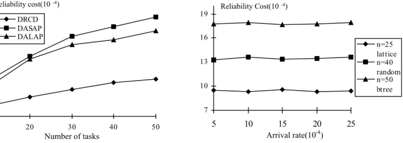
To validate the DRCD algorithm and compare its performance against two existing approaches, we have tested the reliability cost performance of DRCD, DASAP, and DALAP. The benchmark task graphs used for the evaluation include random graphs, binary trees, and lattices. We have chosen this collection of task graphs as a set of benchmarks because they are representative of various applications modeled as directed acyclic graphs. In Figures 2 and 3 we plot reliability cost with increasing job size and job arrival rate. Since results for lattices and random graphs have similar patterns as those for binary tree, we only show results of binary tree in Figure 2.
7 10 13 16 19 5 10 15 20 25 n=25 lattice n=40 random n=50 btree Arrival rate(10-4) Reliability Cost(10-4) 0 5 10 15 20 25 30 35 40 10 20 30 40 50 DRCD DASAP DALAP Number of tasks Reliability cost(10-4)
Fig. 2. Impact of task load on RC. Job aarrival rate = 15*10-4 No./Sec. Binary trees are used.
Fig. 3. Impact of job arrival rate on reliability cost. Binary tree, lattice, and random graphs are used.
Figure 2 shows that, compared with the existing scheduling approaches, DRCD reduces the reliability cost of DASAP and DALAP by up to 71.4% and 66.8% (with average of 63.7% and 61.3%), respectively. The advantage of DRCD over DASAP and DALAP becomes more pronounced as the job size increases. This is expected because DASAP and DALAP do not consider reliability cost as one of their scheduling objectives. DRCD, however, tends to assign tasks to machines on which their reliability cost are minimum.
Another interesting result from this experiment is that job arrival rate seems to have no impact on reliability cost performance. Since DRCD, DASAP and DALAP share the same feature, we only ran DRCD algorithm on three benchmark task graphs. The results shown in Figure 3 indicate that the reliability cost performance depends on job size rather than job arrival rate. This can be attributed to
the fact that the scheduling algorithms employ an admission control strategy, which rejects jobs whose deadlines cannot be guaranteed.
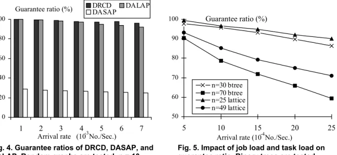
5.3 Guarantee Ratio
In this section we present some experimental results with respect to guarantee ratios. We present two different groups of experimental results based on a set of synthetic benchmarks. First we present performance comparison of the DRCD, DASAP, and DALAP algorithms on a heterogeneous cluster. Second, we illustrate the impact of workload and job size on guarantee ratios.
Fig. 4 shows the results of the experiment where random graphs are used as benchmarks. Results for binary trees and lattices are omitted because they are expected to be similar to those of random graphs. We set the job arrival rate from 1×10⁻³ to 7×10⁻³No./Sec. in increments of 1×10⁻³No./Sec. Figure 4 shows that the guarantee ratio of DRCD is slightly higher than that of the DALAP algorithm, and DRCD significantly outperforms DASAP in terms of guarantee ratio. This is mainly because the resource utilization of DRCD is less than those of DASAP and DALAP. In general, this result can be attributed to the fact that, in an effort to minimize reliability cost, the DRCD approach constantly strives to shorten execution times of each task in a job.
50 60 70 80 90 100 5 10 15 20 25 n=30 btree n=70 btree n=25 lattice n=49 lattice
Arrival rate (10-4No./Sec.)
Guarantee ratio (%) 0 20 40 60 80 100 1 2 3 4 5 6 7 DRCD DALAP DASAP
Arrival rate (10-3No./Sec.) Guarantee ratio (%)
Fig. 4. Guarantee ratios of DRCD, DASAP, and DALAP. Random graphs are tested. n = 10
Fig. 5. Impact of job load and task load on guarantee ratio. Binary trees are tested.
Figure 5 shows the results of the second experiment on two types of benchmark task graphs: binary trees and lattices. For each curve in Figure 5, the number of tasks in each job is fixed, whereas the job arrival rate is changed from 5×10⁻⁴ to 25×10-4 No./Sec. Figures 4 and 5 show the drop in guarantee ratio with increasing values of job arrival rate. Additionally, Figure 5 illustrates that guarantee ratio
decreases as the number of tasks increases. This is because increasing job arrival rate and size results in increased scheduling and dispatching times, which in term give rise to lowered guarantee ratio.
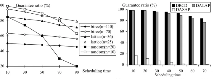
5.4 Scheduling Time
To study the impact of scheduling time on guarantee ratios, we present in this section two sets of experimental results. First, we illustrate the results for the DRCD algorithm in Figure 6. Second, we compare DRCD against DASAP and DALAP with respect to the impact of the scheduling time on their guarantee ratios (See Fig. 7). Although the scheduling time of each job can be estimated as a function of m, n, and u (see Section 5.1 item 4), the scheduling time in this experiment varies from 10 to 90. This simplification deflates any correlations between scheduling times and other workload parameters, but the goal of this simulation is to examine the impact of the scheduling time on system performance by controlling the scheduling time as a parameter.
Fig. 7. Guarantee ratios of the three heuristics when scheduling time is varied. Random graphs
are tested. N = 10, arrival rate is 2*10-3No./Sec.
20 40 60 80 100 10 30 50 70 90 btree(n=110) btree(n=70) lattice(n=36) lattice(n=25) random(n=20) random(n=10) Scheduling time Guarantee ratio (%) 0 20 40 60 80 100 10 20 30 40 50 60 70 DRCD DALAP DASAP Scheduling time Guarantee ratio (%)
Fig. 6. Impact of scheduling time on guarantee ratio. Arrival rate is 2*10-3 No./Sec.
Both binary tree-, lattice- and random graph-based jobs are considered. For each curve in Fig. 6, the job size is fixed and the job arrival rate is set to be 2*10-3No./Sec. Fig. 6 shows guarantee ratio as a function of scheduling time. It reveals that the scheduling time makes significant impact on the performance of a dynamically scheduled real-time heterogeneous cluster. Without considering scheduling time, the predictions on which scheduling is based cannot be accurate, thus lowering GR. This impact is more pronounced as job arrival rate increases. The result also suggests that, under the same workload, shortening the scheduling time can improve guarantee ratios, thus allowing more jobs to be completed before their given deadlines. Ahmad and Kwok have developed a parallel algorithm (referred to as PBSA) that could perform scheduling using multiple processors [2]. Therefore, it is
highly desirable to apply the parallel technique reported in [2] to our algorithm, thereby shortening scheduling time to ultimately enhance the performance of the heterogeneous cluster.
Fig. 7 compares the guarantee ratios of the three heuristics when the scheduling time is varied in this experiment. We find that DRCD can outperform the other alternatives in terms of guarantee ratio, and this finding is consistent with the results shown in Fig. 4. We also observe from Fig. 7 that the guarantee ratios of the DASAP and DALAP algorithms are more sensitive to changes in the scheduling time than DRCD. The result reveals that the improvement in guarantee ratio offered by DRCD becomes more pronounced when the scheduling time is relatively large.
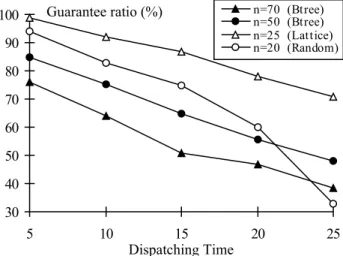
5.5 Dispatching Time
Figure 8 shows the impact of dispatching time of the DRCD algorithm on guarantee ratio for different values of n. Again, job arrival rate is fixed at 2*10-3No./Sec. Dispatching time is increased from 5 to 25 with increments of 5 Sec. Job size is set to 50 and 70 for binary tree, 25 for lattice, and 20 for random graph, respectively. Fig. 8 clearly shows that decreasing dispatching time can significantly improve guarantee ratios of the heterogeneous cluster. This result strongly suggests that using a high-speed network to speed up the dispatching of scheduled tasks can substantially enhance the system performance.
5.6 Heterogeneous Cluster Size
To study the impact of the heterogeneous cluster size m (number of nodes) on the performance of DRCD, we fixed job arrival rate at 10*10-4No./Sec., and increased m from 10 up to 140. Figure 9 shows scheduling time as a function of the heterogeneous cluster size, indicating a noticeable impact
0 5 10 15 20 25 30 35 40 45 20 40 60 80 100 120 140 btree,n=70 btree,n=30 lattice,n=49 lattice,n=36 random,n=70 Number of Nodes Time Compexity (10-4) 30 40 50 60 70 80 90 5 10 15 20 25 n=70 (Btree) n=50 (Btree) n=25 (Lattice) n=20 (Random) Dispatching Time Guarantee ratio (%) 100
Fig. 8. Impact of dispatching time of DRCD
algorithm on GR. Arrival rate is 2*10-3No./Sec. Fig. 9. Impact of the number of nodes on time complexity of the DRCD algorithm.
of both the heterogeneous cluster size (m) and job size (n) on scheduling time. When the job size is small, the impact of m on scheduling time is not very significant. But this impact becomes increasingly noticeable as the job size increases. This is because scheduling time is the product of m,
n and u (Theorem 1).
Figure 10 illustrates the impact of the heterogeneous cluster size on the reliability cost. It shows that under the same workload, the performance with respect to reliability cost improves as the heterogeneous cluster size increases. The main reason behind this is that for a large heterogeneous cluster, the DRCD algorithm has more choices for scheduling a real-time task. It is also observed from Fig. 10 that when the cluster size is more than 30 the improvement in reliability cost starts to diminish. This is because a higher value of m can result in a longer scheduling time (see Fig. 9), especially when the value of n is also high. This result suggests that, under the workload in this experiment, it may not be cost-effective for the system to grow beyond 30 machines. An optimal value of m for a particular workload may be determined by experiments.
40 50 60 70 80 90 100 10 20 30 40 50 60 btree,n=70 btree,n=30 lattice,n=49 lattice,n=25 random, n=30 Number of nodes Guarantee Ratio (%) 2 6 10 14 18 22 10 20 30 40 60 80 100 btree,n=70 btree,n=30 lattice,n=49 lattice,n=25 random,n=40 Number of nodes (m) Reliability cost (10-4)
Fig. 10. Impact of the number of nodes on reliability cost of DRCD. Arrival rate is 1*10-3No./Sec.
Fig. 11. Impact of the number of nodes on guarantee ratio of the DRCD algorithm, arrival rate is 1*10-3No./Sec.
The impact of cluster size on guarantee ratio is shown in Fig. 11, where guarantee ratio is plotted as a function of the number of nodes. The results indicate that the impact of the cluster size on guarantee ratios is mixed. On the negative side, a higher value of m can lead to a longer scheduling time, as illustrated in Fig. 9. On the positive side, increasing the number of machines enhances the computational capability of the system, which may in turn guarantee more jobs to be completed before their deadlines. The final result depends on which side makes more significant impact.
As shown in Fig. 11, three curves illustrate the positive side, and two other curves depict the negative side. We observe that when n (job size) is comparatively low, the net effect is positive (see
the three curves in Fig. 11 with n = 25, n = 30); whereas, the negative effect emerges as n becomes relatively high (see two curves in Fig. 10, with n = 49 and n = 70). This suggests that the number of machines is a critical parameter for scheduling parallel real-time jobs, which must be determined carefully based on experiments.
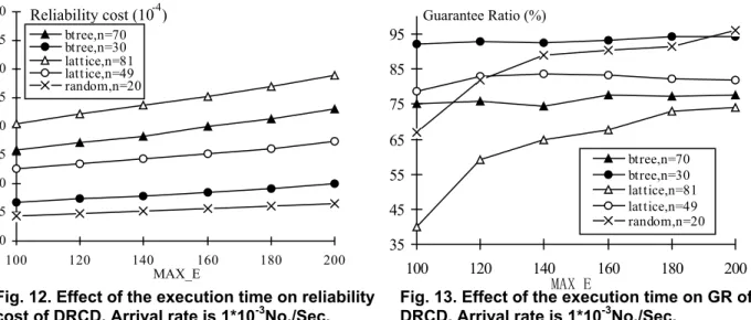
5.7 Execution time
Figure 12 shows the impact of execution time on reliability cost. We only consider the DRCD algorithm, since DASAP and DALAP have similar properties and are less relevant. In this experiment, the job arrival rate is set at 10*10-4No./Sec., and MAX_E is varied from 100 to 200 Sec. with increments of 20 Sec. For each value of MAX_E, we ran the DRDC algorithm on binary trees, lattices and random graphs. From the simulation results shown in Fig. 12, we observe that the reliability cost increases with the increase in the execution time. This is due to the simple fact that when execution time in each cij increases the task reliability cost of machines, RCPN, also increases. We can conclude
from this experiment that as the execution time increases, the reliability cost of the cluster also increases. 0 5 10 15 20 25 30 35 40 100 120 140 160 180 200 btree,n=70 btree,n=30 lattice,n=81 lattice,n=49 random,n=20 MAX_E Reliability cost (10-4)
Fig. 12. Effect of the execution time on reliability cost of DRCD. Arrival rate is 1*10-3No./Sec.
35 45 55 65 75 85 95 100 120 140 160 180 200 btree,n=70 btree,n=30 lattice,n=81 lattice,n=49 random,n=20 MAX E Guarantee Ratio (%)
Fig. 13. Effect of the execution time on GR of DRCD. Arrival rate is 1*10-3No./Sec.
As shown in Fig. 13, execution time also has a noticeable impact on guarantee ratios. When the value of n is low (see the curve with n = 30), execution time does not make a significant impact on guarantee ratio, but when n becomes large (see the curve with n = 81), we observe that guarantee ratios are affected noticeably by the execution time. Since deadline is assumed to be a function of execution time in our simulation model, the deadlines of tasks increase accordingly when execution time increases. More real-time tasks can be guaranteed if their deadlines are relaxed.
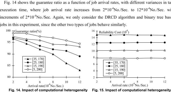
5.8 Computational Heterogeneity
Fig. 14 shows the guarantee ratio as a function of job arrival rates, with different variances in task execution time, where job arrival rate increases from 2*10-4No./Sec. to 12*10-4No./Sec. with increments of 2*10-4No./Sec. Again, we only consider the DRCD algorithm and binary tree based jobs in this experiment, since the other two types of jobs behave similarly.
80 85 90 95 100 2 4 6 8 10 12 [35, 170] [25, 180] [15, 190] [5, 200]
Arrival rate(10-4No./Sec.) Guarantee ratio(%) 2 4 6 8 10 12 14 16 2 4 6 8 10 12 [35, 170] [25, 180] [15, 190] [5, 200]
Arrival rate (10-4No./Sec.) Reliability Cost (10-4)
Fig. 15. Impact of computational heterogeneity on reliability cost. Task graphs are btrees Fig. 14. Impact of computational heterogeneity
on guarantee ratios. Task graphs are btrees
Computational heterogeneity is reflected by the variance in execution times. In the experiment four sets of execution times, all with the same average value, are selected uniformly from the four ranges, [5, 200], [15, 190], [25, 180] and [35, 170], respectively. These four ranges correspond to four different levels of heterogeneity, with [5, 200] being the highest. Fig. 14 and Fig. 15 indicate that the DRCD scheduling algorithm has better performance for jobs with higher computational heterogeneity. This result suggests that high computational heterogeneity helps the DRCD algorithm increase guarantee ratio and reduce reliability cost, thereby enhancing the schedulability. This can be explained by the fact that the advantage of DRCD over the two non-reliability driven algorithms in schedulability mainly comes from the variance in tasks' reliability costs among different machines and reduced heterogeneity implies reduced variance in tasks' reliability costs. It is proved by this experiment that DRCD is efficient in terms of scheduling heterogeneous jobs, and its performance varies with the heterogeneity of the parallel real-time jobs.
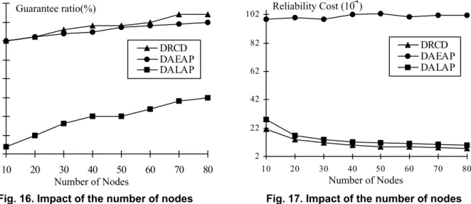
5.9 Performance on Real Applications
The goal of this experiment is two-fold: (1) to validate the results from the synthetic application cases and (2) to test the scalability of the proposed algorithm. We chose a real-life application, a digital signal processing (DSP) system with 119 tasks in the task graph [40], as a case study to
quantitatively evaluate the improvements in guarantee ratio and reliability cost as we increase the number of nodes in the cluster.
60 65 70 75 80 85 90 95 100 10 20 30 40 50 60 70 80 DRCD DAEAP DALAP Number of Nodes Guarantee ratio(%) 2 22 42 62 82 102 10 20 30 40 50 60 70 80 DRCD DAEAP DALAP Number of Nodes Reliability Cost (10-4)
Fig. 17. Impact of the number of nodes on reliability cost for the DSP example Fig. 16. Impact of the number of nodes
on guarantee ratio for the DSP example
We conducted experiments with eight cluster sizes (the number of nodes is varied from 10 to 80). The guarantee ratio and reliability cost were obtained for each heterogeneous cluster, where machine failure rates were randomly chosen between 9.5×10⁻⁷ and 10.5×10⁻⁷/hour and link failure rates between 7.5×10⁻⁶ and 12.5×10⁻⁶/hour. Job arrival rates were kept constant at 1.0×10⁻⁴ No./ms., and ranges for generating deadlines were fixed to 500 ms. Fig. 16 shows the guarantee ratios of the DRCD, DASAP, and DALAP algorithms running on eight heterogeneous clusters. Comparing DRCD with two other algorithms, we find that the DRCD algorithm performances better than the other alternatives, and DRCD improves guarantee ratios over DASAP and DALAP by up to 3% and 45%, respectively. Fig. 17 compares reliability cost for the DRCD, DASAP, and DALAP algorithms. We observe that with respect to reliability cost, DRCD is constantly better than the other two algorithms. Specifically, DRCD can reduce the reliability cost of DASAP and DALAP by up to 92% and 25% (with average of 89% and 21%), respectively. From these results, we conclude that the proposed DRCD algorithm can achieve the most reliable allocations for both small- and large-scale applications by leveraging the reliability-cost driven technique while improving resource utilization.
6. Conclusion
Most research work in the area of real-time task scheduling in heterogeneous systems either ignored reliability issues, or only considered homogeneous clusters, or assumed independent tasks, or only schedule tasks with precedence constraints offline. In this paper, we have addressed these issues
![Fig. 1 depicts the scheduler model in a heterogeneous cluster environment. This model is similar to the one described in [13][14][19][35], where a global scheduler works in concert with a Resource Manager](https://thumb-us.123doks.com/thumbv2/123dok_us/1908592.2779771/6.918.187.709.599.818/depicts-scheduler-heterogeneous-environment-described-scheduler-resource-manager.webp)