Terrence J. Sejnowski and Tomaso A. Poggio, editors
Neural Nets in Electric Fish, Walter Heiligenberg, 1991
The Computational Brain, Patricia S. Churchland and Terrence J. Sejnowski, 1992
Dynamic Biological Networks: The Stomatogastric Nervous System, edited by Ronald M. Harris-Warrick, Eve Marder, Allen I. Selverston, and Maurice Maulins, 1992
The Neurobiology of Neural Networks, edited by Daniel Gardner, 1993
Large-Scale Neuronal Theories of the Brain, edited by Christof Koch and Joel L. Davis, 1994
The Theoretical Foundations of Dendritic Function: Selected Papers of Wilfrid Rall with Commentaries, edited by Idan Segev, John Rinzel, and Gordon M. Shepherd, 1995
Models of Information Processing in the Basal Ganglia, edited by James C. Houk, Joel L. Davis, and David G. Beiser, 1995
Spikes: Exploring the Neural Code, Fred Rieke, David Warland, Rob de Ruyter van Stevenick, and William Bialek, 1997
Neurons, Networks, and Motor Behavior, edited by Paul S. Stein, Sten Grillner, Allen I. Selverston, and Douglas G. Stuart, 1997
Methods in Neuronal Modeling: From Ions to Networks, second edition, edited by Christof Koch and Idan Segev, 1998
Fundamentals of Neural Network Modeling: Neuropsychology and Cognitive Neuroscience, edited by Randolph W. Parks, Daniel S. Levin, and Debra L. Long, 1998
Neural Codes and Distributed Representations: Foundations of Neural Computation, edited by Laurence Abbott and Terrence J. Sejnowski, 1999
Unsupervised Learning: Foundations of Neural Computation, edited by Geoffrey Hinton and Terrence J. Sejnowski, 1999
Fast Oscillations in Cortical Circuits, Roger D. Traub, John G.R. Jefferys, and Miles Al Whittington, 1999
Computational Vision: Information Processing in Perception and Visual Behavior, Hanspeter A. Mallot, 2000
Graphical Models: Foundations of Neural Computation, edited by Michael I. Jordan and Terrence J. Sejnowski, 2001
Self-Organizing Map Formation: Foundation of Neural Computation, edited by Klaus Ober-mayer and Terrence J. Sejnowski, 2001
Theoretical Neuroscience: Computational and Mathematical Modeling of Neural Systems, Peter Dayan and L. F. Abbott, 2001
Neural Engineering: Computation, Representation, and Dynamics in Neurobiological Sys-tems, Chris Eliasmith and Charles H. Anderson, 2003
The Computational Neurobiology of Reaching and Pointing, edited by Reza Shadmehr and Steven P. Wise, 2005
Dynamical Systems in Neuroscience: The Geometry of Excitability and Bursting, Eugene M. Izhikevich, 2007
The Geometry of Excitability and Bursting
Eugene M. Izhikevich
The MIT Press
Cambridge, Massachusetts
London, England
All rights reserved. No part of this book may be reproduced in any form by any elec-tronic or mechanical means (including photocopying, recording, or information storage and retrieval) without permission in writing from the publisher.
MIT Press books may be purchased at special quantity discounts for business or sales promotional use. For information, please [email protected] write to Special Sales Department, The MIT Press, 55 Hayward Street, Cambridge, MA 02142
This book was set in LATEX by the author. Printed and bound in the United States of
America.
Library of Congress Cataloging-in-Publication Data Izhikevich, Eugene M., 1967–
Dynamical systems in neuroscience: the geometry of excitability and bursting / Eugene M. Izhikevich.
p. cm. — (Computational neuroscience) Includes bibliographical references and index. ISBN 978-0-262-09043-8 (hc. : alk. paper)
1. Neural networks (Neurobiology) 2. Neurons - computer simulation. 3. Dy-namical systems. 4. Computational neuroscience. I. Izhikevich, E. M. II Title. III. Series.
QP363.3.I94 2007
573.8’01’13—DC21 2006040349
Contents
Preface xv
1 Introduction 1
1.1 Neurons . . . 1
1.1.1 What Is a Spike? . . . 2
1.1.2 Where Is the Threshold? . . . 3
1.1.3 Why Are Neurons Different, and Why Do We Care? . . . 6
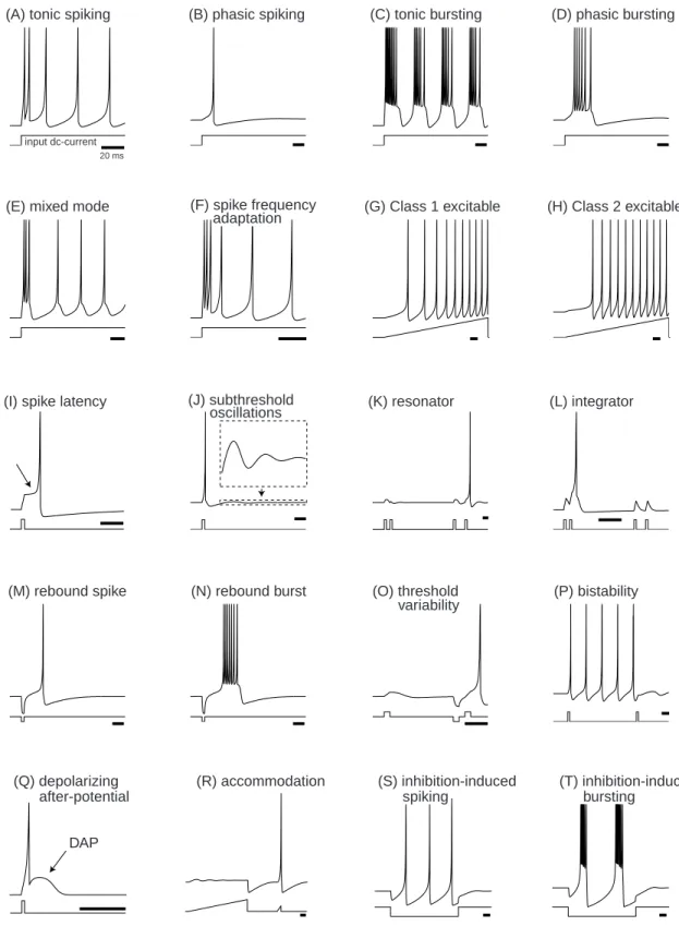
1.1.4 Building Models . . . 6 1.2 Dynamical Systems . . . 8 1.2.1 Phase Portraits . . . 8 1.2.2 Bifurcations . . . 11 1.2.3 Hodgkin Classification . . . 14 1.2.4 Neurocomputational properties . . . 16
1.2.5 Building Models (Revisited) . . . 20
Review of Important Concepts . . . 21
Bibliographical Notes . . . 21
2 Electrophysiology of Neurons 25 2.1 Ions . . . 25
2.1.1 Nernst Potential . . . 26
2.1.2 Ionic Currents and Conductances . . . 27
2.1.3 Equivalent Circuit . . . 28
2.1.4 Resting Potential and Input Resistance . . . 29
2.1.5 Voltage-Clamp and I-V Relation . . . 30
2.2 Conductances . . . 32
2.2.1 Voltage-Gated Channels . . . 33
2.2.2 Activation of Persistent Currents . . . 34
2.2.3 Inactivation of Transient Currents . . . 35
2.2.4 Hyperpolarization-Activated Channels . . . 36
2.3 The Hodgkin-Huxley Model . . . 37
2.3.1 Hodgkin-Huxley Equations . . . 37
2.3.2 Action Potential . . . 41
2.3.3 Propagation of the Action Potentials . . . 42 vii
2.3.4 Dendritic Compartments . . . 43
2.3.5 Summary of Voltage-Gated Currents . . . 44
Review of Important Concepts . . . 49
Bibliographical Notes . . . 50
Exercises . . . 50
3 One-Dimensional Systems 53 3.1 Electrophysiological Examples . . . 53
3.1.1 I-V Relations and Dynamics . . . 54
3.1.2 Leak + InstantaneousINa,p . . . 55 3.2 Dynamical Systems . . . 57 3.2.1 Geometrical Analysis . . . 59 3.2.2 Equilibria . . . 60 3.2.3 Stability . . . 60 3.2.4 Eigenvalues . . . 61 3.2.5 Unstable Equilibria . . . 61 3.2.6 Attraction Domain . . . 62
3.2.7 Threshold and Action Potential . . . 63
3.2.8 Bistability and Hysteresis . . . 66
3.3 Phase Portraits . . . 67
3.3.1 Topological Equivalence . . . 68
3.3.2 Local Equivalence and the Hartman-Grobman Theorem . . . 69
3.3.3 Bifurcations . . . 70
3.3.4 Saddle-Node (Fold) Bifurcation . . . 74
3.3.5 Slow Transition . . . 75
3.3.6 Bifurcation Diagram . . . 77
3.3.7 Bifurcations and I-V Relations . . . 77
3.3.8 Quadratic Integrate-and-Fire Neuron . . . 80
Review of Important Concepts . . . 82
Bibliographical Notes . . . 83
Exercises . . . 83
4 Two-Dimensional Systems 89 4.1 Planar Vector Fields . . . 89
4.1.1 Nullclines . . . 92 4.1.2 Trajectories . . . 94 4.1.3 Limit Cycles . . . 96 4.1.4 Relaxation Oscillators . . . 98 4.2 Equilibria . . . 99 4.2.1 Stability . . . 100
4.2.2 Local Linear Analysis . . . 101
4.2.3 Eigenvalues and Eigenvectors . . . 102
4.2.5 Classification of Equilibria . . . 103
4.2.6 Example: FitzHugh-Nagumo Model . . . 106
4.3 Phase Portraits . . . 108
4.3.1 Bistability and Attraction Domains . . . 108
4.3.2 Stable/Unstable Manifolds . . . 109
4.3.3 Homoclinic/Heteroclinic Trajectories . . . 111
4.3.4 Saddle-Node Bifurcation . . . 113
4.3.5 Andronov-Hopf Bifurcation . . . 116
Review of Important Concepts . . . 121
Bibliographical Notes . . . 122
Exercises . . . 122
5 Conductance-Based Models and Their Reductions 127 5.1 Minimal Models . . . 127
5.1.1 Amplifying and Resonant Gating Variables . . . 129
5.1.2 INa,p+IK-Model . . . 132 5.1.3 INa,t-model . . . 133 5.1.4 INa,p+Ih-Model . . . 136 5.1.5 Ih+IKir-Model . . . 138 5.1.6 IK+IKir-Model . . . 140 5.1.7 IA-Model . . . 142
5.1.8 Ca2+-Gated Minimal Models . . . . 147
5.2 Reduction of Multidimensional Models . . . 147
5.2.1 Hodgkin-Huxley model . . . 147
5.2.2 Equivalent Potentials . . . 151
5.2.3 Nullclines and I-V Relations . . . 151
5.2.4 Reduction to Simple Model . . . 153
Review of Important Concepts . . . 156
Bibliographical Notes . . . 156
Exercises . . . 157
6 Bifurcations 159 6.1 Equilibrium (Rest State) . . . 159
6.1.1 Saddle-Node (Fold) . . . 162
6.1.2 Saddle-Node on Invariant Circle . . . 164
6.1.3 Supercritical Andronov-Hopf . . . 168
6.1.4 Subcritical Andronov-Hopf . . . 174
6.2 Limit Cycle (Spiking State) . . . 178
6.2.1 Saddle-Node on Invariant Circle . . . 180
6.2.2 Supercritical Andronov-Hopf . . . 181
6.2.3 Fold Limit Cycle . . . 181
6.2.4 Homoclinic . . . 185
6.3.1 Three-Dimensional Phase Space . . . 190
6.3.2 Cusp and Pitchfork . . . 192
6.3.3 Bogdanov-Takens . . . 194
6.3.4 Relaxation Oscillators and Canards . . . 198
6.3.5 Bautin . . . 200
6.3.6 Saddle-Node Homoclinic Orbit . . . 201
6.3.7 Hard and Soft Loss of Stability . . . 204
Bibliographical Notes . . . 205 Exercises . . . 210 7 Neuronal Excitability 215 7.1 Excitability . . . 215 7.1.1 Bifurcations . . . 216 7.1.2 Hodgkin’s Classification . . . 218 7.1.3 Classes 1 and 2 . . . 221 7.1.4 Class 3 . . . 222
7.1.5 Ramps, Steps, and Shocks . . . 224
7.1.6 Bistability . . . 226
7.1.7 Class 1 and 2 Spiking . . . 228
7.2 Integrators vs. Resonators . . . 229
7.2.1 Fast Subthreshold Oscillations . . . 230
7.2.2 Frequency Preference and Resonance . . . 232
7.2.3 Frequency Preference in Vivo . . . 237
7.2.4 Thresholds and Action Potentials . . . 238
7.2.5 Threshold manifolds . . . 240
7.2.6 Rheobase . . . 242
7.2.7 Postinhibitory Spike . . . 242
7.2.8 Inhibition-Induced Spiking . . . 244
7.2.9 Spike Latency . . . 246
7.2.10 Flipping from an Integrator to a Resonator . . . 248
7.2.11 Transition Between Integrators and Resonators . . . 251
7.3 Slow Modulation . . . 252
7.3.1 Spike Frequency Modulation . . . 255
7.3.2 I-V Relation . . . 256
7.3.3 Slow Subthreshold Oscillation . . . 258
7.3.4 Rebound Response and Voltage Sag . . . 259
7.3.5 AHP and ADP . . . 260
Review of Important Concepts . . . 264
Bibliographical Notes . . . 264
8 Simple Models 267
8.1 Simplest Models . . . 267
8.1.1 Integrate-and-Fire . . . 268
8.1.2 Resonate-and-Fire . . . 269
8.1.3 Quadratic Integrate-and-Fire . . . 270
8.1.4 Simple Model of Choice . . . 272
8.1.5 Canonical Models . . . 278
8.2 Cortex . . . 281
8.2.1 Regular Spiking (RS) Neurons . . . 282
8.2.2 Intrinsically Bursting (IB) Neurons . . . 288
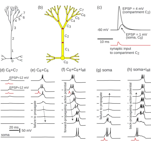
8.2.3 Multi-Compartment Dendritic Tree . . . 292
8.2.4 Chattering (CH) Neurons . . . 294
8.2.5 Low-Threshold Spiking (LTS) Interneurons . . . 296
8.2.6 Fast Spiking (FS) Interneurons . . . 298
8.2.7 Late Spiking (LS) Interneurons . . . 300
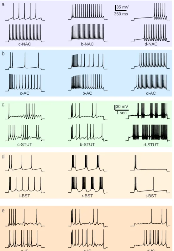
8.2.8 Diversity of Inhibitory Interneurons . . . 301
8.3 Thalamus . . . 304
8.3.1 Thalamocortical (TC) Relay Neurons . . . 305
8.3.2 Reticular Thalamic Nucleus (RTN) Neurons . . . 306
8.3.3 Thalamic Interneurons . . . 308
8.4 Other Interesting Cases . . . 308
8.4.1 Hippocampal CA1 Pyramidal Neurons . . . 308
8.4.2 Spiny Projection Neurons of Neostriatum and Basal Ganglia . . 311
8.4.3 Mesencephalic V Neurons of Brainstem . . . 313
8.4.4 Stellate Cells of Entorhinal Cortex . . . 314
8.4.5 Mitral Neurons of the Olfactory Bulb . . . 316
Review of Important Concepts . . . 319
Bibliographical Notes . . . 319
Exercises . . . 321
9 Bursting 325 9.1 Electrophysiology . . . 325
9.1.1 Example: TheINa,p+IK+IK(M)-Model . . . 327
9.1.2 Fast-Slow Dynamics . . . 329
9.1.3 Minimal Models . . . 332
9.1.4 Central Pattern Generators and Half-Center Oscillators . . . 334
9.2 Geometry . . . 335
9.2.1 Fast-Slow Bursters . . . 336
9.2.2 Phase Portraits . . . 336
9.2.3 Averaging . . . 339
9.2.4 Equivalent Voltage . . . 341
9.2.5 Hysteresis Loops and Slow Waves . . . 342
9.3 Classification . . . 347 9.3.1 Fold/Homoclinic . . . 350 9.3.2 Circle/Circle . . . 354 9.3.3 SubHopf/Fold Cycle . . . 359 9.3.4 Fold/Fold Cycle . . . 364 9.3.5 Fold/Hopf . . . 365 9.3.6 Fold/Circle . . . 366 9.4 Neurocomputational Properties . . . 367 9.4.1 How to Distinguish? . . . 367 9.4.2 Integrators vs. Resonators . . . 368 9.4.3 Bistability . . . 368
9.4.4 Bursts as a Unit of Neuronal Information . . . 371
9.4.5 Chirps . . . 372
9.4.6 Synchronization . . . 373
Review of Important Concepts . . . 375
Bibliographical Notes . . . 376 Exercises . . . 378 10 Synchronization 385 Solutions to Exercises 387 References 419 10 Synchronization (www.izhikevich.com) 435 10.1 Pulsed Coupling . . . 436 10.1.1 Phase of Oscillation . . . 436 10.1.2 Isochrons . . . 437 10.1.3 PRC . . . 438
10.1.4 Type 0 and Type 1 Phase Response . . . 442
10.1.5 Poincare Phase Map . . . 444
10.1.6 Fixed points . . . 445 10.1.7 Synchronization . . . 446 10.1.8 Phase-Locking . . . 448 10.1.9 Arnold Tongues . . . 448 10.2 Weak Coupling . . . 450 10.2.1 Winfree’s Approach . . . 451 10.2.2 Kuramoto’s Approach . . . 452 10.2.3 Malkin’s Approach . . . 453 10.2.4 Measuring PRCs Experimentally . . . 454
10.2.5 Phase Model for Coupled Oscillators . . . 457
10.3 Synchronization . . . 459
10.3.1 Two Oscillators . . . 461
10.3.3 Networks . . . 465 10.3.4 Mean-Field Approximations . . . 466 10.4 Examples . . . 467 10.4.1 Phase Oscillators . . . 467 10.4.2 SNIC Oscillators . . . 469 10.4.3 Homoclinic Oscillators . . . 474
10.4.4 Relaxation Oscillators and FTM . . . 476
10.4.5 Bursting Oscillators . . . 478
Review of Important Concepts . . . 480
Bibliographical Notes . . . 481
Solutions . . . 489
Preface
Historically, much of theoretical neuroscience research concerned neuronal circuits and synaptic organization. The neurons were divided into excitatory and inhibitory types, but their electrophysiological properties were largely neglected or taken to be identical to those of Hodgkin-Huxley’s squid axon. The present awareness of the importance of the electrophysiology of individual neurons is best summarized by David McCormick in the fifth edition of Gordon Shepherd’s bookThe Synaptic Organization of the Brain:
Information-processing depends not only on theanatomical substrates of synap-tic circuits but also on theelectrophysiological properties of neurons... Even if two neurons in different regions of the nervous system possess identical morpho-logical features, they may respond to the same synaptic input in very different manners because of each cell’s intrinsic properties.
McCormick (2004)
Much of present neuroscience research concerns voltage- and second-messenger-gated currents in individual cells, with the goal of understanding the cell’s intrinsic neurocomputational properties. It is widely accepted that knowing the currents suffices to determine what the cell is doing and why it is doing it. This, however, contradicts a half-century–old observation that cells having similar currents can nevertheless exhibit quite different dynamics. Indeed, studying isolated axons having presumably similar electrophysiology (all are from the crustacean Carcinus maenas), Hodgkin (1948) in-jected a DC-current of varying amplitude, and discovered that some preparations could exhibit repetitive spiking with arbitrarily low frequencies, while the others discharged in a narrow frequency band. This observation was largely ignored by the neuroscience community until the seminal paper by Rinzel and Ermentrout (1989), who showed that the difference in behavior is due to differentbifurcation mechanisms of excitability.
Let us treat the amplitude of the injected current in Hodgkin’s experiments as a bifurcation parameter: When the amplitude is small, the cell is quiescent; when the amplitude is large, the cell fires repetitive spikes. When we change the amplitude of the injected current, the cell undergoes a transition from quiescence to repetitive spiking. From the dynamical systems point of view, the transition corresponds to a bifurcation from equilibrium to a limit cycle attractor. The type of bifurcation determines the most fundamental computational properties of neurons, such as the class of excitability, the existence or nonexistence of threshold, all-or-none spikes, subthreshold oscillations, the ability to generate postinhibitory rebound spikes, bistability of resting and spiking states, whether the neuron is an integrator or a resonator, and so on.
This book is devoted to a systematic study of the relationship between electrophysi-ology, bifurcations, and computational properties of neurons. The reader will learn why cells having nearly identical currents may undergo distinct bifurcations, and hence they will have fundamentally different neurocomputational properties. (Conversely, cells
having quite different currents may undergo identical bifurcations, and hence they will have similar neurocomputational properties.) The major message of the book can be summarized as follows (compare with the McCormick statement above):
Information-processing depends not only on the electrophysiological properties of neurons but also on their dynamical properties. Even if two neurons in the same region of the nervous system possess similar electrophysiological features, they may respond to the same synaptic input in very different manners because of each cell’s bifurcation dynamics.
Nonlinear dynamical system theory is a core of computational neuroscience research, but it is not a standard part of the graduate neuroscience curriculum. Neither is it taught in most math/physics departments in a form suitable for a general biological audience. As a result, many neuroscientists fail to grasp such fundamental concepts as equilibrium, stability, limit cycle attractor, and bifurcations, even though neuroscien-tists constantly encounter these nonlinear phenomena.
This book introduces dynamical systems starting with simple one- and two-dimen-sional spiking models and continuing all the way to bursting systems. Each chapter is organized from simple to complex, so everybody can start reading the book; only the reader’s background will determine where he or she stops. The book emphasizes the geometrical approach, so there are few equations but a lot of figures. Half of them are simulations of various neural models, so there are hundreds of possible exercises such as “Use MATLAB (GENESIS, NEURON, XPPAUT, etc.) and parameters in the caption of figure X to simulate the figure.” Additional problems are provided at the end of each chapter; the reader is encouraged to solve at least some of them and to look at the solutions of the others at the end of the book. Problems marked[M.S.]or
[Ph.D.]are suggested thesis topics.
Acknowledgments.
I thank the scientists who reviewed the first draft of the book: Pablo Achard, Jose M. Amigo, Vlatko Becanovic, Brent Doiron, George Bard Ermentrout, Richard FitzHugh, David Golomb, Andrei Iacob, Paul Kulchenko, Maciej Lazarewicz, Georgi Medvedev, John Rinzel, Anil K. Seth, Gautam C Sethia, Arthur Sherman, Klaus M. Stiefel, and Takashi Tateno. I also thank the anonymous refer-ees who peer-reviewed the book and made quite a few valuable suggestions instead of just rejecting it. Special thanks go to Niraj S. Desai, who made most of the in vitro recordings used in the book (the data are available on the author’s Web page www.izhikevich.com), and to Bruno van Swinderen, who drew the cartoons. I en-joyed the hospitality of The Neurosciences Institute – a monastery of interdisciplinary science – and I benefited greatly from the expertise and support of its fellows.Finally, I thank my wife, Tatyana, and my wonderful daughters, Elizabeth and Kate, for their support and patience during the five-year gestation of this book.
Eugene M. Izhikevich www.izhikevich.com
Chapter 1
Introduction
This chapter highlights some of the most important concepts developed in the book. First, we discuss several common misconceptions regarding the spike generation mech-anism of neurons. Our goal is to motivate the reader to think of a neuron not only in terms of ions and channels, as many biologists do, and not only in terms of an in-put/output relationship, as many theoreticians do, but also as a nonlinear dynamical system that looks at the input through the prism of its own intrinsic dynamics. We ask such questions as “What makes a neuron fire?” or “Where is the threshold?”, and then outline the answers, using the geometrical theory of dynamical systems.
From a dynamical systems point of view, neurons are excitable because they are near a transition, called bifurcation, from resting to sustained spiking activity. While there is a huge number of possible ionic mechanisms of excitability and spike genera-tion, there are only four bifurcation mechanisms that can result in such a transition. Considering the geometry of phase portraits at these bifurcations, we can understand many computational properties of neurons, such as the nature of threshold and all-or-none spiking, the coexistence of resting and spiking states, the origin of spike latencies, postinhibitory spikes, and the mechanism of integration and resonance. Moreover, we can understand how these properties are interrelated, why some are equivalent, and why some are mutually exclusive.
1.1
Neurons
If somebody were to put a gun to the head of the author of this book and ask him to name the single most important concept in brain science, he would say it is the concept
of a neuron. There are only 1011 or so neurons in the human brain, much fewer than
the number of non-neural cells such as glia. Yet neurons are unique in the sense that only they can transmit electrical signals over long distances. From the neuronal level we can go down to cell biophysics and to the molecular biology of gene regulation. From the neuronal level we can go up to neuronal circuits, to cortical structures, to the whole brain, and finally to the behavior of the organism. So let us see how much we understand of what is going on at the level of individual neurons.
0.1 mm soma apical dendrites basal dendrites axon synapse 40 ms -60 mV +35 mV spike membrane potential, mV time, ms recording electrode
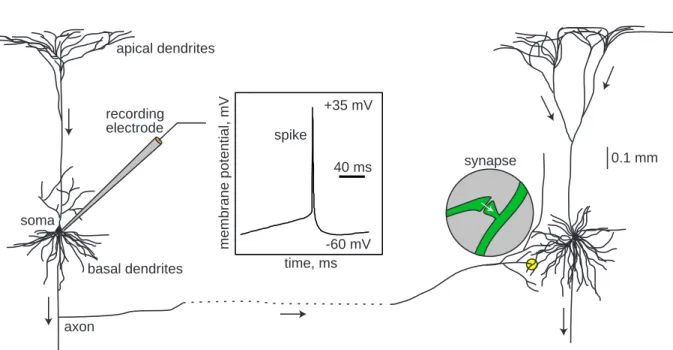
Figure 1.1: Two interconnected cortical pyramidal neurons (hand drawing) and in vitro recorded spike.
1.1.1
What Is a Spike?
A typical neuron receives inputs from more than 10,000 other neurons through the con-tacts on its dendritic tree called synapses; see Fig.1.1. The inputs produce electrical transmembrane currents that change the membrane potential of the neuron. Synaptic currents produce changes, called postsynaptic potentials (PSPs). Small currents pro-duce small PSPs; larger currents propro-duce significant PSPs that can be amplified by the voltage-sensitive channels embedded in the neuronal membrane and lead to the gen-eration of an action potential orspike – an abrupt and transient change of membrane voltage that propagates to other neurons via a long protrusion called an axon.
Such spikes are the main means of communication between neurons. In general, neurons do not fire on their own; they fire as a result of incoming spikes from other neurons. One of the most fundamental questions of neuroscience is What, exactly,
makes neurons fire? What is it in the incoming pulses that elicits a response in one
neuron but not in another? Why can two neurons have different responses to exactly the same input and identical responses to completely different inputs? To answer these questions, we need to understand the dynamics of spike generation mechanisms of neurons.
Most introductory neuroscience books describe neurons as integrators with a thresh-old: neurons sum incoming PSPs and “compare” the integrated PSP with a certain voltage value, called the firing threshold. If it is below the threshold, the neuron re-mains quiescent; when it is above the threshold, the neuron fires an all-or-none spike, as in Fig.1.3, and resets its membrane potential. To add theoretical plausibility to this argument, the books refer to the Hodgkin-Huxley model of spike generation in squid
Figure 1.2: What makes a neuron fire?
giant axons, which we study in chapter 2. The irony is that the Hodgkin-Huxley model does not have a well-defined threshold; it does not fire all-or-none spikes; and it is not an integrator, but a resonator (i.e., it prefers inputs having certain frequencies that resonate with the frequency of subthreshold oscillations of the neuron). We consider these and other properties in detail in this book.
1.1.2
Where Is the Threshold?
Much effort has been spent trying to experimentally determine the firing thresholds of neurons. Here, we challenge the classical view of a threshold. Let us consider two typical experiments, depicted in Fig.1.4, that are designed to measure the threshold. in Fig.1.4a, we shock a cortical neuron (i.e., we inject brief but strong pulses of current of various amplitudes to depolarize the membrane potential to various values). Is there a clear-cut voltage value, as in Fig.1.3, above which the neuron fires but below which no spikes occur? If you find one, let the author know! In Fig.1.4b we inject long but weak pulses of current of various amplitudes, which results in slow depolarization and a spike. The firing threshold, if it exists, must be somewhere in the shaded region, but where? Where does the slow depolarization end and the spike start? Is it meaningful to talk about firing thresholds at all?
resting threshold
all-or-none spikes
no spike
-40 mV
1 ms 20 mV
injected pulses of current
spikes subthreshold response 15 ms spikes cut (a) (b) threshold?
injected pulses of current
Figure 1.4: Where is the firing threshold? Shown are in vitro recordings of two layer 5 rat pyramidal neurons. Notice the differences of voltage and time scales.
-60 mV 20 mV 100 ms (a) (b) 20 mV 5 ms
Figure 1.5: Where is the rheobase (i.e., the minimal current that fires the cell)? (a) in vitro recordings of the pyramidal neuron of layer 2/3 of a rat’s visual cortex show increasing latencies as the amplitude of the injected current decreases. (b) Simulation of the INa,p+IK– model (pronounced: persistent sodium plus potassium model) shows
spikes of graded amplitude.
Perhaps, we should measure current thresholds instead of voltage thresholds. The current threshold (i.e., the minimal amplitude of injected current of infinite duration needed to fire a neuron) is called the rheobase. In Fig.1.5 we decrease the amplitudes of injected pulses of current to find the minimal one that still elicits a spike or the maximal one that does not. In Fig.1.5a, progressively weaker pulses result in longer latencies to the first spike. Eventually the neuron does not fire because the latency is longer than the duration of the pulse, which is 1 second in the figure. Did we really measure the neuronal rheobase? What if we waited a bit longer? How long is long enough? In Fig.1.5b the latencies do not grow, but the spike amplitudes decrease until the spikes do not look like spikes at all. To determine the current threshold, we need to draw the line and separate spike responses from “subthreshold” ones. How can we do that if the spikes are not all-or-none? Is the response denoted by the dashed line a spike?
Risking adding more confusion to the notion of a threshold, consider the follow-ing. If excitatory inputs depolarize the membrane potential (i.e., bring it closer to
-45 mV
10 mV 10 ms
-100 pA 0 pA
Figure 1.6: In vitro recording of rebound spikes of a rat’s brainstem mesV neuron in response to a brief hyperpolarizing pulse of current.
5ms 10ms
resonant burst
non-resonant burst inhibitory burst
10ms 15ms
non-resonant burst
Figure 1.7: Resonant response of the mesencephalic V neuron of a rat’s brainstem to pulses of injected current having a 10 ms period (in vitro).
the “firing threshold”), and inhibitory inputs hyperpolarize the potential and move it away from the threshold, then how can the neuron in Fig.1.6 fire in response to the
inhibitory input? This phenomenon, also observed in the Hodgkin-Huxley model, is
called anodal break excitation, rebound spike, or postinhibitory spike. Many biolo-gists say that rebound responses are due to the activation and inactivation of certain slow currents, which bring the membrane potential over the threshold or, equivalently, lower the threshold upon release from the hyperpolarization – a phenomenon called a low-threshold spike in thalamocortical neurons. The problem with this explanation is that neither the Hodgkin-Huxley model nor the neuron in Fig.1.6 has these currents, and even if they did, the hyperpolarization is too short and too weak to affect the currents.
Another interesting phenomenon is depicted in Fig.1.7. The neuron is stimulated with brief pulses of current mimicking an incoming burst of three spikes. When the stimulation frequency is high (5 ms period), presumably reflecting a strong input, the neuron does not fire at all. However, stimulation with a lower frequency (10 ms period) that resonates with the frequency of subthreshold oscillation of the neuron evokes a spike response, regardless of whether the stimulation is excitatory or inhibitory. Stimulation with even lower frequency (15 ms period) cannot elicit spike response again. Thus, the neuron is sensitive only to the inputs having resonant frequency. The same pulses applied to a cortical pyramidal neuron evoke a response only in the first case (small period), but not in the other cases.
1.1.3
Why Are Neurons Different, and Why Do We Care?
Why would two neurons respond completely differently to the same input? A biologist would say that the response of a neuron depends on many factors, such as the type of voltage- and Ca2+-gated channels expressed by the neuron, the morphology of itsdendritic tree, the location of the input, and other factors. These factors are indeed important, but they do not determine the neuronal response per se. Rather they determine the rules that govern dynamics of the neuron. Different conductances and currents can result in the same rules, and hence in the same responses; conversely, similar currents can result in different rules and in different responses. The currents define what kind of dynamical system the neuron is.
We study ionic transmembrane currents in chapter 2. In subsequent chapters we investigate how the types of currents determine neuronal dynamics. We divide all cur-rents into two major classes: amplifying and resonant, with the persistent Na+current INa,p and the persistent K+ current IK being the typical examples of the former and
the latter, respectively. Since there are tens of known currents, purely combinatorial argument implies that there are millions of different electrophysiological mechanisms of spike generation. We will show later that any such mechanism must have at least one amplifying and one resonant current. Some mechanisms, called minimal in this book, have one resonant and one amplifying current. They provide an invaluable tool in classifying and understanding the electrophysiology of spike generation.
Many illustrations in this book are based on simulations of the reducedINa,p+IK
-model (pronounced persistent sodium plus potassium model), which consists of a fast persistent Na+ (amplifying) current and a slower persistent K+ (resonant) current. It
is equivalent to the famous and widely used Morris-Lecar ICa+IK-model (Morris and Lecar 1981). We show that the model exhibits quite different dynamics, depending on the values of the parameters, e.g., the half-activation voltage of the K+ current: in one
case, it can fire in a narrow frequency range, it can exhibit coexistence of resting and spiking states, and it has damped subthreshold oscillations of membrane potential. In another case, it can fire in a wide frequency range and show no coexistence of resting and spiking and no subthreshold oscillations. Thus, seemingly inessential differences in parameter values could result in drastically distinct behaviors.
1.1.4
Building Models
To build a good model of a neuron, electrophysiologists apply different pharmacologi-cal blockers to tease out the currents that the neuron has. Then they apply different stimulation protocols to measure the kinetic parameters of the currents, such as the Boltzmann activation function, time constants, and maximal conductances. We con-sider all these functions in chapter 2. Next, they create a Hodgkin-Huxley-type model and simulate it using the NEURON, GENESIS, or XPP environment or MATLAB (the first two are invaluable tools for simulating realistic dendritic structures).
The problem is that the parameters are measured in different neurons and then put together into a single model. As an illustration, consider two neurons having the same
Figure 1.8: Neurons are dynamical systems.
currents, sayINa,p and IK, and exhibiting excitable behavior; that is, both neurons are
quiescent but can fire a spike in response to a stimulation. Suppose the second neuron has stronger INa,p, which is balanced by stronger IK. If we measure Na+ conductance
using the first neuron and K+ conductance using the second neuron, the resulting INa,p+IK-model will have an excess of K+ current and probably will not be able to fire
spikes at all. Conversely, if we measure Na+ and K+ conductances using the second
neuron and then the first neuron, respectively, the model would have too much Na+
current and probably would exhibit sustained pacemaking activity. In any case, the model fails to reproduce the excitable behavior of the neurons whose parameters we measured.
Some of the parameters cannot be measured at all, so many arbitrary choices are made via a process called “fine-tuning”. Navigating in the dark, possibly with the help of some biological intuition, the researcher modifies parameters, compares simulations with experiment, and repeats this trial-and-error procedure until he or she is satisfied with the results. Since seemingly similar values of parameters can result in drastically different behaviors, and quite different parameters can result in seemingly similar be-haviors, how do we know that the resulting model is correct? How do we know that its behavior is equivalent to that of the neuron we want to study? And what isequivalent
1.2
Dynamical Systems
In chapter 2 we introduce the Hodgkin-Huxley formalism to describe neuronal dynamics in terms of activation and inactivation of voltage-gated conductances. An important result of the Hodgkin-Huxley studies is that neurons are dynamical systems, so they should be studied as such. Below we mention some of the important concepts of dynamical systems theory. The reader does not have to follow all the details of this section because the concepts are explained in greater detail in subsequent chapters.
A dynamical system consists of a set of variables that describe its state and a law that describes the evolution of the state variables with time (i.e., how the state of the system in the next moment of time depends on the input and its state in the previous moment of time). The Hodgkin-Huxley model is a four-dimensional dynamical system because its state is uniquely determined by the membrane potential,V, and so-called gating variables n, m, and h for persistent K+ and transient Na+ currents. The
evolution law is given by a four-dimensional system of ordinary differential equations. Typically, all variables describing neuronal dynamics can be classified into four classes, according to their function and the time scale.
1. Membrane potential.
2. Excitation variables, such as activation of a Na+ current. These variables are
responsible for the upstroke of the spike.
3. Recovery variables, such as inactivation of a Na+ current and activation of a fast
K+ current. These variables are responsible for the repolarization (downstroke)
of the spike.
4. Adaptation variables, such as activation of slow voltage- or Ca2+-dependent
cur-rents. These variables build up during prolonged spiking and can affect excitabil-ity in the long run.
The Hodgkin-Huxley model does not have variables of the fourth type, but many neuronal models do, especially those exhibiting bursting dynamics.
1.2.1
Phase Portraits
The power of the dynamical systems approach to neuroscience, as well as to many other sciences, is that we can tell something, or many things, about a system without knowing all the details that govern the system evolution. We do not even use equations to do that! Some may even wonder why we call it a mathematical theory.
As a start, let us consider a quiescent neuron whose membrane potential is rest-ing. From the dynamical systems point of view, there are no changes of the state variables of such a neuron; hence it is at an equilibrium point. All the inward currents that depolarize the neuron are balanced, or equilibrated, by the outward currents that hyperpolarize it. If the neuron remains quiescent despite small disturbances and mem-brane noise, as in Fig.1.9a (top), then we conclude that the equilibrium is stable. Isn’t
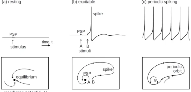
(a) resting (b) excitable (c) periodic spiking equilibrium spike spike periodic orbit stimulus stimuli membrane potential, V K + activation gate, n
membrane potential, V(t) time, t
A B
A B PSP PSP PSP
Figure 1.9: Resting, excitable, and periodic spiking activity correspond to a stable equilibrium (a and b) or limit cycle (c), respectively.
it amazing that we can reach such a conclusion without knowing the equations that describe the neuron’s dynamics? We do not even know the number of variables needed to describe the neuron; it could be infinite, for all we care.
In this book we introduce the notions of equilibria, stability, threshold, and attrac-tion domains using one- and two-dimensional dynamical systems, e.g., the INa,p+IK
-model with instantaneous Na+ kinetics. The state of this model is described by the
membrane potential,V, and the activation variable,n, of the persistent K+ current, so
it is a two-dimensional vector (V, n). Instantaneous activation of the Na+ current is a
function ofV, so it does not result in a separate variable of the model. The evolution of the model is a trajectory (V(t), n(t)) on the V ×n– plane. Depending on the initial point, the system can have many trajectories, such as those depicted in Fig.1.9a (bot-tom). Time is not explicitly present in the figure, but units of time may be thought of as plotted along each trajectory. All of the trajectories in the figure are attracted to the stable equilibrium denoted by the black dot, called an attractor. The overall qualitative description of dynamics can be obtained through the study of the phase portrait of the system, which depicts certain special trajectories (equilibria, separatri-ces, limit cycles) that determine the topological behavior of all the other trajectories in the phase space. Probably 50 percent of illustrations in this book are phase portraits. A fundamental property of neurons is excitability, illustrated in Fig.1.9b. The neu-ron is resting, i.e., its phase portrait has a stable equilibrium. Small perturbations, such as A, result in small excursions from the equilibrium, denoted as PSP (postsynap-tic potential). Larger perturbations, such as B, are amplified by the neuron’s intrinsic dynamics and result in the spike response. To understand the dynamic mechanism of such amplification, we need to consider the geometry of the phase portrait near the resting equilibrium, i.e., in the region where the decision to fire or not to fire is made.
resting mode spiking
mode
Figure 1.10: Rhythmic transitions between resting and spiking modes result in bursting behavior. 20 mV 500 ms -60 mV 0 pA 0 pA 3000 pA -50 mV 200 pA transition transition
layer 5 pyramidal cell brainstem mesV cell
500 ms
Figure 1.11: As the magnitude of the injected current slowly increases, the neurons bifurcate from resting (equilibrium) mode to tonic spiking (limit cycle) mode.
If we inject a sufficiently strong current into the neuron, we bring it to a pacemaking mode, so that it exhibits periodic spiking activity, as in Fig.1.9c. From the dynamical systems point of view, the state of such a neuron has a stable limit cycle, also known as a stable periodic orbit. The electrophysiological details of the neuron (i.e., the number and the type of currents it has, their kinetics, etc.) determine only the location, the shape, and the period of the limit cycle. As long as the limit cycle exists, the neuron can have periodic spiking activity. Of course, equilibria and limit cycles can coexist, so a neuron can be switched from one mode to another by a transient input. The famous example is the permanent extinguishing of ongoing spiking activity in the squid giant axon by a brief transient depolarizing pulse of current applied at a proper phase (Guttman et al. 1980) – a phenomenon predicted by John Rinzel (1978) purely on the basis of theoretical analysis of the Hodgkin-Huxley model. The transition between resting and spiking modes could be triggered by intrinsic slow conductances, resulting in the bursting behavior in Fig.1.10.
1.2.2
Bifurcations
Now suppose that the magnitude of the injected current is a parameter that we can control, e.g., we can ramp it up, as in Fig.1.11. Each cell in the figure is quiescent at the beginning of the ramps, so its phase portrait has a stable equilibrium and it may look like the one in Fig.1.9a or Fig.1.9b. Then it starts to fire tonic spikes, so its phase portrait has a limit cycle attractor and it may look like the one in Fig.1.9c, with a white circle denoting an unstable resting equilibrium. Apparently there is some intermediate level of injected current that corresponds to the transition from resting to sustained spiking, i.e., from the phase portrait in Fig.1.9b to Fig.1.9c. What does the transition look like?
From the dynamical systems point of view, the transition corresponds to a bifurca-tion of neuron dynamics, i.e., a qualitative change of phase portrait of the system. For example, there is no bifurcation going from the phase portrait in Fig.1.9a to that in Fig.1.9b, since both have one globally stable equilibrium; the difference in behavior is quantitative but not qualitative. In contrast, there is a bifurcation going from Fig.1.9b to Fig.1.9c, since the equilibrium is no longer stable and another attractor, limit cycle, has appeared. The neuron is not excitable in Fig.1.9a but it is in Fig.1.9b, simply because the former phase portrait is far from the bifurcation and the latter is near.
In general, neurons are excitable because they are near bifurcations from resting to spiking activity, so the type of the bifurcation determines the excitable properties of the neuron. Of course, the type depends on the neuron’s electrophysiology. An amazing observation is that there could be millions of different electrophysiological mechanisms of excitability and spiking, but there are only four – yes, four – different types of bifurcations of equilibrium that a system can undergo without any additional constraints, such as symmetry. Thus, considering these four bifurcations in a general setup, we can understand excitable properties of many models, even those that have not been invented yet. What is even more amazing, we can understand excitable properties of neurons whose currents are not measured and whose models are not known, provided we can experimentally identify which of the four bifurcations the resting state of the neuron undergoes.
The four bifurcations are summarized in Fig.1.12, which plots the phase portrait before (left), at (center), and after (right) a particular bifurcation occurs. Mathemati-cians refer to these bifurcations as being of codimension-1 because we need to vary only one parameter, e.g., the magnitude of the injected DC currentI, to observe the bifur-cations reliably in simulations or experiments. There are many more codimension-2, 3, (etc.), bifurcations, but they need special conditions to be observed. We discuss these in chapter 6.
Let us consider the four bifurcations and their phase portraits in Fig.1.12. The horizontal and vertical axes are the membrane potential with instantaneous activation variable and a recovery variable, respectively. At this stage, the reader is not required to fully understand the intricacies of the phase portraits in the figure, since they will be explained systematically in later chapters.
saddle-node node saddle
node saddle saddle-node
inva
riant c
ircle
saddle-node on invariant circle (SNIC) bifurcation saddle-node bifurcation
subcritical Andronov-Hopf bifurcation
supercritical Andronov-Hopf bifurcation
(a) (b) (c) (d) sp ikin glim itcy cle
spiking limit cycleatt
ra c to r uns table reco v er y potential
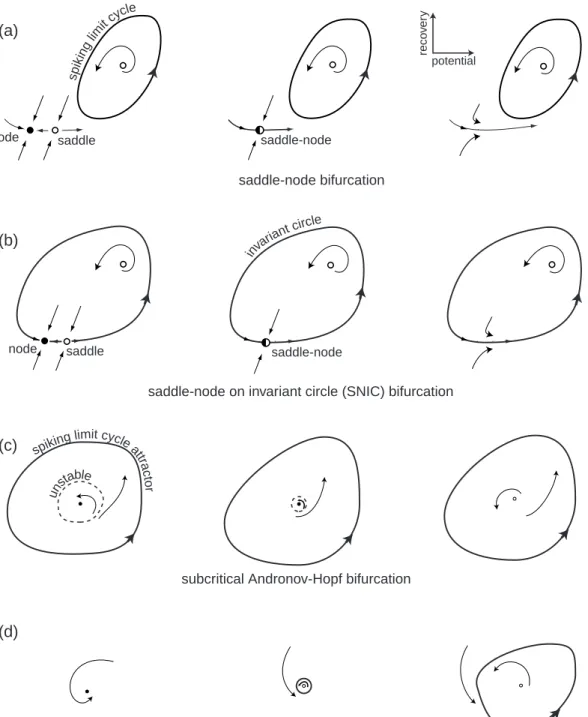
Figure 1.12: Four generic (codimension-1) bifurcations of an equilibrium state leading to the transition from resting to periodic spiking behavior in neurons.
• Saddle-node bifurcation. As the magnitude of the injected current or any other bifurcation parameter changes, a stable equilibrium corresponding to the resting state (black circle marked “node” in Fig.1.12a) is approached by an unstable equilibrium (white circle marked “saddle”); they coalesce and annihilate each other, as in Fig.1.12a (middle). Since the resting state no longer exists, the tra-jectory describing the evolution of the system jumps to the limit cycle attractor, indicating that the neuron starts to fire tonic spikes. Notice that the limit cy-cle, or some other attractor, must coexist with the resting state in order for the transition resting→ spiking to occur.
• Saddle-node on invariant circle bifurcationis similar to the saddle-node bifurca-tion except that there is an invariant circle at the moment of bifurcabifurca-tion, which then becomes a limit cycle attractor, as in Fig.1.12b.
• Subcritical Andronov-Hopf bifurcation. A small unstable limit cycle shrinks to
a stable equilibrium and makes it lose stability, as in Fig.1.12c. Because of instabilities, the trajectory diverges from the equilibrium and approaches a large-amplitude spiking limit cycle or some other attractor.
• Supercritical Andronov-Hopf bifurcation. The stable equilibrium loses stability
and gives birth to a small-amplitude limit cycle attractor, as in Fig.1.12d. As the magnitude of the injected current increases, the amplitude of the limit cycle increases and it becomes a full-size spiking limit cycle.
Notice that there is a coexistence of resting and spiking states in the case of saddle-node and subcritical Andronov-Hopf bifurcations, but not in the other two cases. Such a coexistence reveals itself via a hysteresis behavior when the injected current slowly increases and then decreases past the bifurcation value, because the transitions “resting →spiking” and “spiking→resting” occur at different values of the current. In addition, brief stimuli applied at the appropriate times can switch the activity from spiking to resting and back. There are also spontaneous noise-induced transitions between the two modes that result in the stuttering spiking that, for instance, is exhibited by the so-called fast spiking (FS) cortical interneurons when they are kept close to the bifurcation (Tateno et al. 2004). Some bistable neurons have a slow adaptation current that activates during the spiking mode and impedes spiking, often resulting in bursting activity.
Systems undergoing Andronov-Hopf bifurcations, whether subcritical or supercrit-ical, exhibit damped oscillations of membrane potential, whereas systems near saddle-node bifurcations, whether on or off an invariant circle, do not. The existence of small amplitude oscillations creates the possibility of resonance to the frequency of the incoming pulses, as in Fig.1.7, and other interesting features.
We refer to neurons with damped subthreshold oscillations as resonators and to those that do not have this property as integrators. We refer to the neurons that ex-hibit the coexistence of resting and spiking states, at least near the transition from
coexistence of resting and spiking states YES (bistable) NO (monostable) subthreshold oscillations YES (resonator) NO (integ
rator) saddle-node saddle-node on
invariant circle
subcritical Andronov-Hopf
supercritical Andronov-Hopf
Figure 1.13: Classification of neurons into monostable/bistable integrators/resonators according to the bifurcation of the resting state in Fig.1.12. 0 500 1000 1500 0 50 100 150 200 250 0 100 200 300 0 10 20 30 40
injected dc-current, I (pA) injected dc-current, I (pA)
asymptotic fir ing frequency , Hz asymptotic fir ing frequency , Hz F-I curve F-I curve Class 1 excitability Class 2 excitability
Figure 1.14: Frequency-current (F-I) curves of cortical pyramidal neuron and brainstem mesV neuron from Fig.7.3. These are the same neurons used in the ramp experiment in Fig.1.11.
resting to spiking, as bistable, and to those that do not, monostable. The four bifur-cations in Fig.1.12 are uniquely defined by these two features. For example, a bistable resonator is a neuron undergoing subcritical Andronov-Hopf bifurcation, and a monos-table integrator is a neuron undergoing saddle-node on invariant circle bifurcation (see Fig.1.13). Cortical fast spiking (FS) and regular spiking (RS) neurons, studied in chapter 8, are typical examples of the former and the latter, respectively.
1.2.3
Hodgkin Classification
Hodgkin (1948) was the first to study bifurcations in neuronal dynamics, years before the mathematical theory of bifurcations was developed. He stimulated squid axons with pulses of various amplitudes and identified three classes of responses:
• Class 1 neural excitability. Action potentials can be generated with arbitrarily
low frequency, depending on the strength of the applied current.
• Class 2 neural excitability. Action potentials are generated in a certain frequency band that is relatively insensitive to changes in the strength of the applied current.
• Class 3 neural excitability. A single action potential is generated in response to a pulse of current. Repetitive (tonic) spiking can be generated only for extremely strong injected currents or not at all.
The qualitative distinction between the classes is that the frequency-current relation (the F-I curve in Fig.1.14) starts from zero and continuously increases for Class 1 neurons, is discontinuous for Class 2 neurons, and is not defined at all for Class 3 neurons.
Obviously, neurons belonging to different classes have different neurocomputational properties. Class 1 neurons, which include cortical excitatory pyramidal neurons, can smoothly encode the strength of the input into the output firing frequency, as in Fig.1.11 (left). In contrast, Class 2 neurons, such as fast-spiking (FS) cortical in-hibitory interneurons, cannot do that; instead, they fire in a relatively narrow frequency band, as in Fig.1.11 (right). Class 3 neurons cannot exhibit sustained spiking activ-ity, so Hodgkin regarded them as “sick” or “unhealthy”. There are other distinctions between the classes, which we discuss later.
Different classes of excitability occur because neurons have different bifurcations of resting and spiking states – a phenomenon first explained by Rinzel and Ermen-trout (1989). If ramps of current are injected to measure the F-I curves, then Class 1 excitability occurs when the neuron undergoes the saddle-node bifurcation on an invariant circle depicted in Fig.1.12b. Indeed, the period of the limit cycle attractor is infinite at the bifurcation point, and then it decreases as the bifurcation parameter – say, the magnitude of the injected current – increases. The other three bifurcations result in Class 2 excitability. Indeed, the limit cycle attractor exists and has a finite period when the resting state in Fig.1.12 undergoes a subcritical Andronov-Hopf bi-furcation, so emerging spiking has a nonzero frequency. The period of the small limit cycle attractor appearing via supercritical Andronov-Hopf bifurcation is also finite, so the frequency of oscillations is nonzero, but their amplitudes are small. In contrast to the common and erroneous folklore, the saddle-node bifurcation (off-limit cycle) also results in Class 2 excitability because the limit cycle has a finite period at the bifurcation. There is a considerable latency (delay) to the first spike in this case, but the subsequent spiking has nonzero frequency. Thus, the simple scheme “Class 1 = saddle-node, Class 2 = Hopf” that permeates many publications is unfortunately incorrect.
When pulses of current are used to measure the F-I curve, as in Hodgkin’s exper-iments, the firing frequency depends on factors besides the type of the bifurcation of the resting state. In particular, low-frequency firing can be observed in systems near Andronov-Hopf bifurcations, as we show in chapter 7. To avoid possible confusion, we define the class of excitability only on the basis of slow ramp experiments.
Hodgkin’s classification has an important historical value, but it is of little use for the dynamic description of a neuron, since naming a class of excitability of a neuron does not tell much about the bifurcations of the resting state. Indeed, it says only that saddle-node on invariant circle bifurcation (Class 1) is different from the other three bifurcations (Class 2), and only when ramps are injected. Dividing neurons into
integrators and resonators with bistable or monostable activity is more informative, so we adopt the classification in Fig.1.13 in this book. In this classification, a Class 1 neuron is a monostable integrator, whereas a Class 2 neuron can be a bistable integrator or a resonator.
1.2.4
Neurocomputational properties
Using the same arrangement as in Fig.1.13, we depict typical geometry of phase portraits near the four bifurcations in Fig.1.15. Let us use the portraits to explain what happens “near the threshold”, i.e., near the place where the decision to fire or not to fire is made. To simplify our geometrical analysis, we assume here that neurons receive shock inputs, i.e., brief but strong pulses of current that do not change the phase portraits, but only push or reset the state of the neuron into various regions of the phase space. We consider these and other cases in detail in chapter 7.
The horizontal axis in each plot in Fig.1.15 corresponds to the membrane potential
V with instantaneous Na+current, and the vertical axis corresponds to a recovery
vari-able, say activation of K+ current. Black circles denote stable equilibria corresponding
to the neuronal resting state. Spiking limit cycle attractors correspond to sustained spiking states, which exist in the two cases depicted in the left half of the figure corre-sponding to the bistable dynamics. The limit cycles are surrounded by shaded regions – their attraction domains. The white region is the attraction domain of the equilib-rium. To initiate spiking, the external input should push the state of the system into the shaded region, and to extinguish spiking, the input should push the state back into the white region.
There are no limit cycles in the two cases depicted in the right half of the figure, so the entire phase space is the attraction domain of the stable equilibrium, and the dynamics are monostable. However, if the trajectory starts in the shaded region, it makes a large-amplitude rotation before returning to the equilibrium – a transient spike. Apparently, to elicit such a spike, the input should push the state of the system into the shaded region.
Now let us contrast the upper and lower halves of the figure, corresponding to integrators and resonators, respectively. We distinguish these two modes of operation on the basis of the existence of subthreshold oscillations near the equilibrium.
First, let us show that inhibition impedes spiking in integrators, but can promote it in resonators. In the integrator, the shaded region is in the depolarized voltage range, i.e., to the right of the equilibrium. Excitatory inputs push the state of the system toward the shaded region, while inhibitory inputs push it away. In resonators, both excitation and inhibition push the state toward the shaded region, because the region wraps around the equilibrium and can be reached along any direction. This explains the rebound spiking phenomenon depicted in Fig.1.6.
Integrators have all-or-none spikes; resonators may not. Indeed, any trajectory
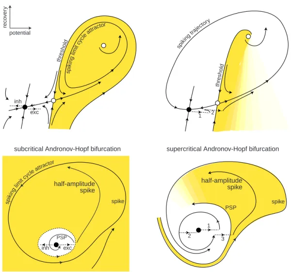
inh sp ikin glim itcy cle attra ctor thre sh old spik ing traje ctory thre sh old exc inh spik ing limit cycle attrac tor 1 2 1 2 3 spike PSP exc
saddle-node bifurcation saddle-node on invariant circle bifurcation
subcritical Andronov-Hopf bifurcation supercritical Andronov-Hopf bifurcation
spike half-amplitude spike half-amplitude spike PSP reco v er y potential
Figure 1.15: The geometry of phase portraits of excitable systems near four bifurcations can explain many neurocomputational properties (see section 1.2.4 for details).
white circle at the top that corresponds to an unstable equilibrium. Moreover, the state of the system is quickly attracted to the spiking trajectory and moves along that trajectory, thereby generating a stereotypical spike. A resonator neuron also can fire large amplitude spikes when its state is pushed to or beyond the trajectory denoted “spike”. Such neurons generate subthreshold responses when the state slides along the smaller trajectory denoted PSP; they also can generate spikes of an intermediate amplitude when the state is pushed between the PSP and “spike” trajectories, which explains the partial-amplitude spiking in Fig.1.5b or in the squid axon in Fig.7.26. The set of initial conditions corresponding to such spiking is quite small, so typical spikes have large amplitudes and partial spikes are rare.
Integrators have well-defined thresholds; resonators may not. The white circles near the resting states of integrators in Fig.1.15 are called saddles. They are stable along the
vertical direction and unstable along the horizontal direction. The two trajectories that lead to the saddle along the vertical direction are called separatrices because they separate the phase space into two regions – in this case, white and shaded. The separatrices play the role of thresholds since only those perturbations that push the state of the system beyond them result in a spike. The closer the state of the system is to the separatrices, the longer it takes to converge and then diverge from the saddle, resulting in a long latency to the spike. Notice that the threshold is not a point, but a tilted curve that spans a range of voltage values.
Resonators have a well-defined threshold in the case of subcritical Andronov-Hopf bifurcation: it is the small unstable limit cycle that separates the attraction domains of stable equilibrium and spiking limit cycle. Trajectories inside the small cycle spi-ral toward the stable equilibrium, whereas trajectories outside the cycle spispi-ral away from it and eventually lead to sustained spiking activity. When a neuronal model is far from the subcritical Andronov-Hopf bifurcation, its phase portrait may look sim-ilar to the one corresponding to the supercritical Andronov-Hopf bifurcation. The narrow shaded band in the figure is not a threshold manifold but a fuzzy thresh-old set called “quasi-threshthresh-old” by FitzHugh (1955). Many resonators, including the Hodgkin-Huxley model, have quasi-thresholds instead of thresholds. The width of the quasi-threshold in the Hodgkin-Huxley model is so narrow that for all practical reasons it may be assumed to be just a curve.
Integrators integrate, resonators resonate. Now consider inputs consisting of multi-ple pulses, e.g., a burst of spikes. Integrators prefer high-frequency inputs; the higher the frequency, the sooner they fire. Indeed, the first spike of such an input, marked “1” in the top-right phase portrait in Fig.1.15, increases the membrane potential and shifts the state to the right, toward the threshold. Since the state of the system is still in the white area, it slowly converges back to the stable equilibrium. To cross the threshold manifold, the second pulse must arrive shortly after the first one. The reaction of a resonator to a pair of pulses is quite different. The first pulse initiates a damped subthreshold oscillation of the membrane potential, which looks like a spiral in the bottom-right phase portrait in Fig.1.15. The effect of the second pulse depends on its timing. If it arrives after the trajectory makes half a rotation, marked “2” in the figure, it cancels the effect of the first pulse. If it arrives after the trajectory makes a full rotation, marked “3” in the figure, it adds to the first pulse and either increases the amplitude of subthreshold oscillation or evokes a spike response. Thus, the response of the resonator neuron depends on the frequency content of the input, as in Fig.1.7.
Integrators and resonators constitute two major modes of activity of neurons. Most cortical pyramidal neurons, including the regular spiking (RS), intrinsically bursting (IB), and chattering (CH) types considered in Chap. 8, are integrators. So are thalam-ocortical neurons in the relay mode of firing, and neostriatal spiny projection neurons. Most cortical inhibitory interneurons, including the FS type, are resonators. So are brainstem mesencephalic V neurons and stellate neurons of the entorhinal cortex. Some cortical pyramidal neurons and low-threshold spiking (LTS) interneurons can be at the border of transition between integrator and resonator modes. Such a transition
corre-spike
Figure 1.16: Phase portrait of a system near a Bogdanov-Takens bifurcation that corresponds to the transition from integrator to resonator mode.
sponds to another bifurcation, which has codimension-2, and hence it is less likely to be encountered experimentally. We consider this and other uncommon bifurcations in detail later. The phase portrait near the bifurcation is depicted in Fig.1.16, and it is a good exercise for the reader to explain why such a system has damped oscillations and postinhibitory responses, yet a well-defined threshold, all-or-none spikes, and possibly long latencies.
Of course, figures 1.15 and 1.16 cannot encompass all the richness of neuronal behav-ior, otherwise this book would be only 19pages long (this book is actually quite short; most of the space is taken by figures, exercises, and solutions). Many aspects of neu-ronal dynamics depend on other bifurcations, e.g., those corresponding to appearance and disappearance of spiking limit cycles. These bifurcations describe the transitions from spiking to resting, and they are especially important when we consider bursting activity. In addition, we need to take into account the relative geometry of equilibria, limit cycles, and other relevant trajectories, and how they depend on the parameters of the system, such as maximal conductances, and activation time constants. We explore all these issues systematically in subsequent chapters.
In chapter 2 we review some of the most fundamental concepts of neuron elec-trophysiology, culminating with the Hodgkin-Huxley model. This chapter is aimed at mathematicians learning neuroscience. In chapters 3 and 4 we use one- and two-dimensional neuronal models, respectively, to review some of the most fundamental concepts of dynamical systems, such as equilibria, limit cycles, stability, attraction domain, nullclines, phase portrait, and bifurcation. The material in these chapters, aimed at biologists learning the language of dynamical systems, is presented with the emphasis on geometrical rather than mathematical intuition. In fact, the spirit of the entire book is to explain concepts by using pictures, not equations. Chapter 5 explores phase portraits of various conductance-based models and the relations be-tween ionic currents and dynamic behavior. In Chapter 6 we use the INa,p+IK-model
to systematically introduce the geometric bifurcation theory. Chapter 7, probably the most important chapter of the book, applies the theory to explain many computational properties of neurons. In fact, all the material in the previous chapters is given so that the reader can understand this chapter. In chapter 8 we use a simple phenomenological
model to simulate many cortical, hippocampal, and thalamic neurons. This chapter contains probably the most comprehensive up-to-date review of various firing patterns exhibited by mammalian neurons. In chapter 9 we introduce the electrophysiological and topological classification of bursting dynamics, as well as some useful methods to study the bursters. Finally, the last and the most mathematically advanced chapter of the book, Chap. 10, deals with coupled neurons. There we show how the details of the spike generation mechanism of neurons affect neurons’ collective properties, such as synchronization.
1.2.5
Building Models (Revisited)
To have a good model of a neuron, it is not enough to put the right kind of currents together and tune the parameters so that the model can fire spikes. It is not even enough to reproduce the right input resistance, rheobase, and firing frequencies. The model has to reproduce all the neurocomputational features of the neuron, starting with the coexistence of resting and spiking states, spike latencies, subthreshold oscillations, and rebound spikes, among others.
A good way to start is to determine what kind of bifurcations the neuron under consideration undergoes and how the bifurcations depend on neuromodulators and pharmacological blockers. Instead of or in addition to measuring neuronal responses to get the kinetic parameters, we need to measure them to get the right bifurcation behavior. Only in this case we can be sure that the behavior of the model isequivalent
to that of the neuron, even if we omitted a current or guessed some of the parameters incorrectly.
Implementation of this research program is still a pipe dream. The people who understand the mathematical aspects of neuron dynamics – those who see beyond conductances and currents – usually do not have the opportunity to do experiments. Conversely, those who study neurons in vitro or in vivo on a daily basis – those who see spiking, bursting, and oscillations; those who can manipulate the experimental setup to test practically any aspect of neuronal activity – do not usually see the value of studying phase portraits, bifurcations, and nonlinear dynamics in general. One of the goals of this book is to change this state and bring these two groups of people closer together.
Review of Important Concepts
• Neurons are dynamical systems.• The resting state of neurons corresponds to a stable equilibrium; the tonic spiking state corresponds to a limit cycle attractor.
• Neurons are excitable because the equilibrium is near a bifurcation.
• There are many ionic mechanisms of spike generation, but only four generic bifurcations of equilibria.
• These bifurcations divide neurons into four categories: integrators or resonators, monostable or bistable.
• Analyses of phase portraits at bifurcations explain why some neu-rons have well-defined thresholds, all-or-none spikes, postinhibitory spikes, frequency preference, hysteresis, and so on, while others do not.
• These features, and not ionic currents per se, determine the neuronal responses, i.e., the kind of computations neurons do.
• A good neuronal model must reproduce not only electrophysiology but also the bifurcation dynamics of neurons.
Bibliographical Notes
Richard FitzHugh at the National Institutes of Health (NIH) pioneered the phase plane analysis of neuronal models with the view to understanding their neurocomputational properties. He was the first to analyze the Hodgkin-Huxley model (FitzHugh 1955; years before they received the Nobel Prize) and to prove that it has neither threshold nor all-or-none spikes. FitzHugh (1961) introduced the simplified model of excitability (see Fig.1.18) and showed that one can get the right kind of neuronal dynamics in mod-els lacking conductances and currents. Nagumo et al. (1962) designed a corresponding tunnel diode circuit, so the model is called the FitzHugh-Nagumo oscillator. Chapter 8 deals with such simplified models. The history of the development of FitzHugh-Nagumo model is reviewed by Izhikevich and FitzHugh (2006).
FitzHugh’s research program was further developed by John Rinzel and G. Bard Ermentrout (see Fig.1.19 and Fig.1.20). In their 1989 seminal paper, Rinzel and Er-mentrout revived Hodgkin’s classification of excitability and pointed out the connection between the behavior of neuronal models and the bifurcations they exhibit. (They also referred to the excitability as “type I” or “type II”). Unfortunately, many people treat
Figure 1.17: Richard FitzHugh in 1984. -2.5 -2 -1.5 -1 -0.5 0 0.5 1 1.5 2 -1 0.5 0 0.5 1 membrane potential, V recovery variable, W W=V-V 3 /3+I W=( V+.7 )/.8 NO MAN'S LAND re la tive ly re frac to ry regenerative a ctiv e resting depolarized quasi-thres hold self-excitatory hyperpolarized absolutely refractory
Figure 1.18: Phase portrait and physiological state diagram of FitzHugh-Nagumo model ˙V = V −V3/3−W +I, ˙W = 0.08(V + 0.7−0.8W). The meaning of curves
and trajectories is explained in chapter 4. (Reproduced from Izhikevich and FitzHugh (2006) with permission.)
Figure 1.19: John Rinzel in 2004. Depicted on his T-shirt is the cover of the first issue of Journal of Computational Neuroscience, in which the Pinsky-Rinzel (1994) model appeared.
Figure 1.20: G. Bard Ermentrout (G. stands for George) with his parrot, Junior, in 1983.
the connection in a simpleminded fashion and incorrectly identify “type I = saddle-node, type II = Hopf”. If only life were so simple!
The geometrical analysis of neuronal models was further developed by, among oth-ers, Izhikevich (2000a), who stressed the integrator and resonator modes of operation and made connections to other neurocomputational properties.
The neuroscience and mathematics parts of this book are standard, though many connections are new. The literature sources are listed at the end of each chapter. Among many outstanding books on computational neuroscience, the author especially recommends Spikes, Decisions, and Actions by Wilson (1999), Biophysics of
Com-putation by Koch (1999), Theoretical Neuroscience by Dayan and Abbott (2001), and
Foundations of Cellular Neurophysiologyby Johnston and Wu (1995). The present
vol-ume complements these excellent books in the sense that it is more ambitious, focused, and thorough in dealing with neurons as dynamical systems. Though its views may be biased by the author’s philosophy and taste, the payoffs in understanding neuronal dynamics are immense, provided the reader has enough patience and perseverance to follow the author’s line of thought.
The NEURON simulation environment is described by Hines (1989) and Carnevale and Hines (2006) (http://www.neuron.yale.edu); the GENESIS environment, by Bower and Beeman (1995) (http://www.genesis-sim.org); the XPP environment, by Ermentrout (2002). The author of this book uses MATLAB, which has become a standard computational tool in science and engineering. MATLAB is the registered trademark of The MathWorks, Inc. (http://www.mathworks.com).