Jean Claude Garreau and Véronique Zehnlé
Université de Lille, CNRS, UMR 8523 - PhLAM - Laboratoire de Physique des Lasers Atomes et Molécules, F-59000 Lille, France∗
(Dated: December 21, 2020)
We present a general model allowing “quantum simulation” of one-dimensional Dirac models with 2- and 4-component spinors using ultracold atoms in driven 1D tilted optical latices. The resulting Dirac physics is illustrated by one of its well-known manifestations, Zitterbewegung. This general model can be extended and applied with great flexibility to more complex situations.
I. INTRODUCTION
The Dirac theory of the electron (with its quantum-electrodynamical corrections) is the most complete, pre-cise, and experimentally well-tested theory in physics. It combines quantum mechanics and relativistic covari-ance in a general frame, automatically including the spin degree of freedom, and predicting the existence of the positron. However, in atomic physics, anda fortiori in cold-atom physics, Dirac theory has played a relatively restricted role, because, experimentally, its domain of ap-plication (v∼c) is not often attained (except for inner-shell electrons of heavy atoms) and, theoretically, many of its important results (e.g. fine structure) can be calcu-lated with a good precision in the simpler frame of Pauli theory (that is, Schrödinger equation plus spin 1/2), at least for light atoms.
Recently, quantum simulation [1] became a mastream in ultracold-atom physics [2]. The basic idea, in-spired by early Feynman insights [3], is to generate the physical behavior corresponding to some model, e.g. con-densed matter’s Hubbard Hamiltonians, by “artificially” creating a corresponding Hamiltonian in more controlled conditions, e.g. ultracold atoms in optical lattices [4]. This “Hamiltonian engineering” has been pushed quite far, with the introduction of artificial gauge fields [5], spin-orbit couplings and Dirac equation simulations [6– 9], quantum magnetism of neutral atoms [10, 11], and the physics of disordered systems [12–16].
Quantum simulation of Dirac physics has benefit of a large interest in recent years. This can be done in con-densed matter systems by taking advantage of the flexible concept of quasi-particles, where in particular the Weyl semimetal [17] is a pertinent concept, and recently the ex-istence of “type-II” Weyl particles (that is a Weyl particle breaking Lorentz isotropy) [18] has been suggested. Dirac quantum simulators using ion traps have also been pro-posed [19]. Another popular way of quantum-simulating Dirac physics is by using ultracold atoms in optical lat-tices, pioneered by Gerritsma et al. [6, 20], who stud-ied the phenomenon of Klein tunneling, also studstud-ied in refs. [7, 8, 21]. Without trying to be exhaustive, a wealth of interesting related phenomena can also be studied:
∗www.phlam.univ-lille1.fr/atfr/cq
topological insulators, Dirac cones, spin-orbit coupling, and even cyclotron dynamics [22–28].
The present work combines these two driving forces in the ultracold-atom field. We propose a general method for simulating Dirac physics in a “tilted” one-dimensional optical lattice, a system that has been very useful since the early days of the quantum simulation (even before the term quantum simulation was introduced), for ex-ample for the observation of Bloch oscillations or the (equivalent) Wannier-Stark ladder [29–35]. The realiza-tion of such a system can be obtained by applying a far-detuned laser standing wave that ultracold atoms see as a sinusoidal potential acting on their center of mass vari-ables [36]. If the atom’s de Broglie wavelength is compa-rable to the lattice constanta=λL/2, whereλL= 2π/kL is the radiation wavelength (we use sans serif symbols for dimensioned quantities), the system is in the quantum regime, a condition easily realized for temperatures of the order of a fewµK. In order to obtain a tilted poten-tial, one can simply chirp one of the beams forming the standing wave: A linear shift of the frequency produces a quadratic displacement of the nodes of the standing wave; in the rest frame with respect to the nodes, an inertial constant force creates a tilt, that is, a poten-tial of the form Vws(x) = −V1cos(2kLx) +Fx, withV1
proportional to the radiation intensity andF(constant) proportional to the frequency chirp. This kind of setup is by now quite common in cold atom physics. In what follows, we shall use dimensionless units such that spa-tial coordinatex=x/ais measured in units of the lattice potential step a, energy in units of the so-called “recoil energy” ER = ~2kL2/2M (M is the mass of the atom), time in units of~/ER;m∗=π2/2is a reduced mass, and ~= 1is the reduced Planck constant [37]. This defines
the (dimensionless)Wannier-Stark Hamiltonian
H0=
p2
x
2m∗ −V1cos(2πx) +F x, (1)
withF ≡Fa/ERandV1=V1/ER. A given well (labeled
by its positionx=n) may, depending onV1andF, host a
number of bound eigenstates, called Wannier-Stark (WS) states [38]. We note ϕ`
n(x) the `th bounded state of welln[39] (see Fig. 1), with the corresponding eigenen-ergy En`. The WS potential Vws= −V1cos(2πx) +F x
of Eq. (1) is invariant under a simultaneous spatial translation by an integer multiplem of the lattice con-stant a = 1 and an energy shift of mF, implying that
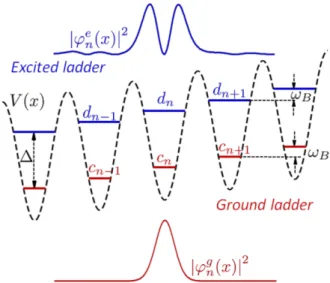
Figure 1. The Wannier-Stark system. Red energy levelsEg n
and amplitude cn form the “ground” Wannier-Stark ladder, the corresponding spatial probability distribution |ϕgn(x)|2 (for site n) is shown as the bottom red curve. Blue levels of energy Ene and amplitude dn form the “excited” WS
lad-der and the corresponding eigenstate|ϕen(x)|2 is shown as the top blue curve. Levels in the same well are separated by an energy∆and levels in the same ladder are separated byωB, the Bloch frequency. The parameters used in this work are
V1= 6,F = 1, for which one finds numerically∆ = 5.66.
ϕ`
n+m(x) =ϕ`n(x−m)and En`+m=En` +mωB. These eigenenergies form the so-calledWannier-Stark ladder of stepωB =F, calledBloch frequency (=|F|a/~in
dimen-sioned units). In the present work we shall consider at most two such ladders: The ground ladder`=gof lowest energy and the first excited ladder`=e.
A perturbation (for example a temporal or spatial modulation of V1 or F), creates couplings between WS
states and may generate interesting dynamics [31, 37, 40– 42]. The aim of the present work is to take advantage of these possibilities to quantum-simulate Dirac dynamics. By an adequate choice of these temporal modulations one can obtain either a spinor-2 model or a spinor-4 Dirac equation.
After a brief summary of the Dirac equation in sec. II, sec. III introduces the general frame of our study; the spinor-2 model and spinor-4 models are described in sec. IV and in sec. V respectively. Section VI discusses the experimental feasibility of our theoretical proposals and Sec. VII draws general conclusions of this work.
Compared to other works demonstrating ways to sim-ulate Dirac physics, an advantage of our method is its simplicity both from the experimental and the theoret-ical point of view. We use simple 1D optical lattices modulated in time, for which analytic calculations can be pushed quite far. The system is realizable experimen-tally with state-of-the-art techniques (see Sec. VI). In particular, no Raman or Zeeman transitions are neces-sary. Moreover, the approach developed here is general and can be easily adapted to different situations, as it
will be seen below (and in future works).
II. THE DIRAC EQUATION IN A NUTSHELL
The Dirac equation governs massive spin-1/2 parti-cles [43, 44]. As shown by Dirac, the requirement for relativistic invariance leads to the existence of spin and antiparticles; the theory deals with aspinor-4, that is, a 4-component state vector whose components are them-selves wave functions:
ψ= ψ1(x, t) ψ2(x, t) ψ3(x, t) ψ4(x, t) .
A possible representation for the Dirac equation for free particles of massmisHψ=i∂tψ, with the Dirac Hamil-tonian
H = α·pc+βmc2 (2)
whereαj (j =x, y, z) andβ are Dirac matrices
αj= 0 σj σj 0 , β= 1 0 0 −1
withσj the Pauli matrices, 1the2×2 identity matrix, pj =−i∂/∂xj (xj =x, y, z) the momentum operator, c the velocity of light, and ~ = 1. For massive particles, in the rest frame of reference, the two upper components of the spinor-4 can be identified with the spin compo-nents of the (positive rest energy state) “particle” and the two bottom components with the spin of the “an-tiparticle” (negative rest energy state), but in a frame in which the particle is in motion, the components are mixed and no such distinction is possible; a spinor-4 de-scription is necessary. However this “contamination” is small if p mc. The general eigenvalues of the Dirac Hamiltonian are± p2c2+m2c41/2
, the distinction be-tween positive and negative eigenstates thus subsists (for a free particle) in all cases.
For a massive free particle, if the momentum is paral-lel to the spin, that is in the z direction (the arbitrary quantization axis for the spin), then the Dirac equation couplesψ1 to ψ3 andψ2 to ψ4. If the momentum is
or-thogonal to the spin (i.e. along thex- or they-axis), it couplesψ1to ψ4andψ2 toψ3. Therefore, in both cases
the quantum dynamics can be described by two spinor-2, obeying decoupled, equivalent equations. We can thus, for instance in the latter case, form thespinor-2
¯ ψ= ψ2 ψ3
which, from Eq. (2), obeys the spinor-2 Dirac equation
where j = x or j = y. A similar equation holds for
(ψ1, ψ4). In presence of a magnetic field, however, the
quantization axis is imposed by the field and for an arbi-trary direction of the momentump, the four components are coupled and the particle is described by a true spinor-4.
Equation (2) is the original Hamiltonian written by Dirac. This representation is well adapted to the case p mc, where the first term is small compared to the second; if the first term is neglected, the Hamiltonian is diagonal. Other representations exist, e.g., the so-called Weyl representation corresponds to the Hamiltonian
HW =c σ·p 0 0 −σ·p +γ0mc2. (4) with γ0= 0 1 1 0 .
This representation is well suited for the ultra-relativistic limitpmc, where the mass termγ0mc2 in Eq. (4)
be-comes much smaller than the first one; neglecting the mass term leaves a diagonal form. For massless particles, the system separates into two subsets of equivalent equa-tions, and can be described by a spinor-2, the so-called Weyl fermion. The above form implies that these parti-cles are characterized by a well-defined projection of the spin along the particle’s momentumσ·p/|p|, a quantity called, as for photons,helicity.
III. GENERAL MODEL
In this section we introduce the general model leading from Wannier-Stark Hamiltonians of the form Eq. (1) to Dirac-like Hamiltonians. We shall consider a restricted state space of one or two ladders, i.e one or two WS states per potential well; the ground WS state (indexed by`=
g)ϕg
n(x) = hx|ϕgniin the well n, of energyEng =nωB, and the first excited WS state (` = e) ϕen(x) of energy Ene = Eng + ∆= nωB + ∆ of same well n where ∆ is the energy offset betweengandelevels in the same well (cf. Fig. 1). We assume in the following that none of these eigenenergies are degenerate.
The general evolution of an arbitrary wave function can then be written in the form
Ψ(x, t) =X n [cn(t) exp (−iEngt)ϕ g n(x) +dn(t) exp (−iEnet)ϕ e n(x)] (5) withcn(0) =hϕg n |Ψ(0)ianddn(0) =hϕ e n|Ψ(0)i. We introduce a perturbationH¯(t)so that our complete Hamiltonian becomesH =H0+ ¯H(t), with
¯
H(t) =−V1cos(2πx)f1(t)+V2cos(πx)f2(t)+VS(x). (6)
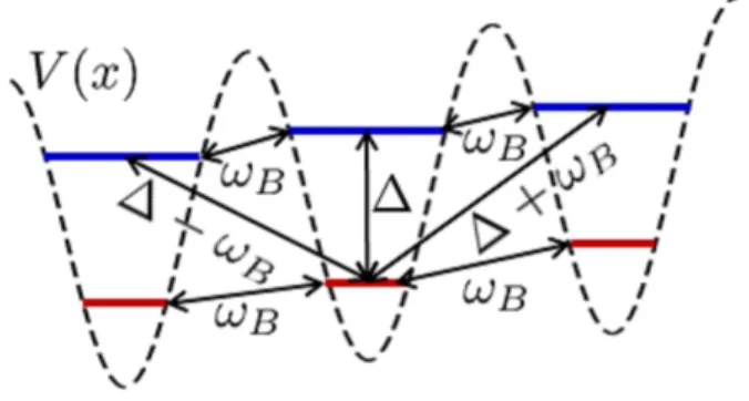
Figure 2. Energy levels and couplings in the Wannier-Stark system. A modulation of frequency ωB induces an intra-ladder coupling between adjacent wells. Inter-ladder cou-plings are induced by perturbation frequencies∆−ωB (n→
n−1),∆(n→n), and∆ +ωB (n→n+ 1).
A suitable choice of the frequencies present inf1(t)and
f2(t) induces interactions between states that are
reso-nantly coupled, as shown in Fig. 2. For example, the ground-ladder level|ϕg
niis resonantly coupled to excited-ladder levelϕen+1
by a modulation of frequency∆+ωB, and toϕen−1
by a modulation of frequency∆−ωB, and so on. The perturbation termV2(x, t) =V2cos(πx)f2(t)
has double spatial period, andVS(x)is a static contribu-tion whose utility will appear below.
Under the action ofH¯ the coupled equations of motion for the amplitudescnanddn of Eq. (5) are developed in App. A and have the form:
id dtcn = X r∈Z hϕg n|H¯ ϕ g n+r e−irωBtcn +r +hϕg n|H¯ ϕen+r e−irωBte−i∆td n+r id dtdn = X r∈Z hϕe n|H¯ ϕ g n+r e−irωBtei∆tcn +r +hϕe n|H¯ ϕen+r e−irωBtdn +r . (7) The functionsfα(t)(α= 1,2) appearing in H, contain¯ modulation frequencies of the formωj,q=jωB+q4with j∈Zandq= 0,±1
fα(t) =X
j,q
A(j,qα)eijωBteiq∆t (8)
where the reality condition implies A(j,qα) = A−(αj,)∗−q. A great advantage of the Wannier-Stark model, within the assumption that parameters are such that there are no intrinsically degenerated states, is that tuning the am-plitudes A(j,qα) allows us to choose which pairs of states are coupled, providing a very flexible control of the dy-namics. For instance, one sees that modulations with q= 0induce intra-ladder couplings (g−gande−e) and modulations with q =±1 induce inter-ladder couplings e−g; takingj= 0creates a couplingg−e in thesame well, whereasj= 1 couples wellsn→n+ 1 andj=−1
In the resonant case, Eqs. (7) can be formally written as id dtcn= X r Tn,rggcn+r+Tn,rgedn+r id dtdn= X r Tn,reedn+r+Tn,regcn+r (9)
(see App. A). The explicit form of coupling coefficients Tab
n,r (a, b∈ {e, g}) between the sitesnandn+rdepend on the overlap integrals, which, thanks to the properties of the WS states, are
hϕg,e n |cos(2πx) ϕ g,e n+r
=hϕg,e0 |cos(2πx)|ϕg,e r i, hϕg,e n |cos(πx) ϕ g,e n+r
= (−1)nhϕg,e0 |cos(πx)|ϕg,e r i. One then obtains intra-ladder coupling as
Tn,rgg =hϕgn|VS|ϕgniδr,0−V1A (1) r,0hϕ g 0|cos(2πx)|ϕ g ri + (−1)nV2A (2) r,0hϕ g 0|cos(πx)|ϕ g ri Tn,ree =hϕen|VS|ϕeniδr,0−V1A (1) r,0hϕ e 0|cos(2πx)|ϕeri + (−1)nV2A (2) r,0hϕ e 0|cos(πx)|ϕ e ri. (10)
and inter-ladder couplings
Tn,rge =−V1A (1) r,1hϕ g 0|cos(2πx)|ϕ e ri + (−1)nV2A (2) r,1hϕ g 0|cos(πx)|ϕ e ri Tn,reg =−V1A (1) r,−1hϕ e 0|cos(2πx)|ϕgri + (−1)nV2A (2) r,−1hϕ e 0|cos(πx)|ϕ g ri. (11) This general model spans all cases we will consider in the present work. In Sec. IV we show how to construct a quantum simulator for a spinor-2 Dirac equation, and in Sec. V we show how the full spinor-4 Dirac or Weyl equations can be synthesized.
IV. SPINOR-2 MODEL
Many interesting phenomena related to the Dirac equa-tion can be illustrated with a simpler spinor-2. In order to construct a spinor-2 quantum simulator we restrict our system to the ground state ladder with “self” (cncn) and nearest neighbors (cn cn±1) couplings.
Inter-ladder transitions are set off by keeping only the q = 0
term in Eq. (8), and we start with an initial condition dn(0) = 0 for all sites [45], so that the excited ladder is never populated. We also setV1=VS = 0in Eq. (6). The
perturbation thus contains only contributions of double spatial period
¯
H =V2f2(t) cos(πx) (12)
with, in Eq. (8),j= 0,±1,q= 0, that is
f2(t) =A (2) 0,0+A (2) 1,0e iωBt+A(2) −1,0e −iωBt =A0+A1eiωBt+A∗1e− iωBt, (13)
where, in the second line, we suppressed for simplicity the fixed indexesq= 0 andα= 2. The remaining coupling parameters are then [Eq. (10)]
Tn,gg1= (−1)nV2A1hϕ g 0|cos(πx)|ϕ g 1i Tn,gg0= (−1)nV2A0hϕ g 0|cos(πx)|ϕ g 0i Tn,gg−1= (−1)nV2A−1hϕg0|cos(πx) ϕ g −1 =−(−1)nV2A∗1hϕ g 0|cos(πx)|ϕ g 1i.
Eqs. (9) then imply
id dtcn=(−1) nV 2A0hϕ g 0|cos(πx)|ϕ g 0icn (−1)nV2hϕ g 0|cos(πx)|ϕ g 1i[A1cn+1−A∗1cn−1]. (14) A key point for realizing a spinor-2 system is that the perturbation of double spatial period creates alternate sign couplings from site to site (see App. A). This has a dynamical effect that is clearly visible in the reciprocal space, where we define “spin” states as “odd site” and “even site” amplitudes
¯ c+(k, t) = X n e2inkc2n(t) ¯ c−(k, t) = X n ei(2n+1)kc2n+1(t). (15)
Taking, for simplicity, A1 real in Eq. (14), one obtains
the following coupled set of equations
id
dtc¯+(k, t) =E0c¯+(k, t)−2iΩ2sink¯c−(k, t) id
dtc¯−(k, t) =−E0¯c−(k, t) + 2iΩ2sink¯c+(k, t), (16)
where we defined the frequency
Ω2 =V2A1hϕ
g
0|cos(πx)|ϕ
g
1i and the “self-energy”
E0 =V2A0hϕ
g
0|cos(πx)|ϕ
g
0i. These two equations show
the emergence of an effective pseudo spinor-2 which in k-space is ¯ ψ= c+(k, t) c−(k, t) .
Looking for solutions inexp (−iω(k)t), the corresponding eigenenergiesω(k)are ω±(k) =± q E2 0+ 4Ω 2 2sin 2k. (17) For E0 = 0, the positive and negative eigenenergies
±2|Ω2sink|are associated to the eigenspinor
¯ ψ±=√1 2 1 ±isgn(Ω2k) , (18)
where sgn(x) is the sign function. The linear, phonon-like, dispersion relation for k → 0 , ω±(k) = ±2|Ω2k|,
reproduces the spectrum of the relativistic massless spin-1/2 fermion. A “1D-conical intersection” occurs as the two branches coalesce atk= 0, creating a so-calledDirac point.
In real space, if the even- c2n(x, t) and odd-site c2n+1(x, t)amplitudes vary slowly on the scale of the
lat-tice step a = 1, one can take the continuous limit of Eqs. (14), and define the functions c±(x, t) as the
spa-tial envelopes of thecn(x, t)(cf. App. A), leading to the spinor-2 φ= c+(x, t) c−(x, t)
which obeys an equation
i∂tφ=−2Ω2(−i∂x)σyφ+E0σzφ (19)
of the same form as Eq. (3) if one setspy =−i∂x(the la-beling of the axes is obviously arbitrary). By comparing Eqs. (19) and (2) we can make the following identifica-tions: E0 =mc2 and2|Ω2|=c, wherem andc are the
effective mass and speed of light which can be adjusted by changing the modulation amplitudes A0 and A1 in
Eq. (13).
The validity of the model Eq. (16) can be numerically tested by comparison with the simulation of the exact Schrödinger equation corresponding to the Hamiltonian H0+ ¯H with H¯ given by Eq. (12). We chose a broad
initial wave packet, with amplitudes:
c2n=a+G(k0)(2n), c2n+1 (20)
=a−G(k0)(2n+ 1), (21)
with G(k0)(n) = (2π/σ)1/2exp (−ink
0)exp −n2/σ2,
σ1,with the normalization condition|a+|2+|a−|2= 1. The initial spinor is thus
φ0= a+ a− G(k0)(x)↔ a+ a− ¯ G(k0)(k) (22)
where the first expression is in real and the second in mo-mentum space, and G¯(k0)(k)is a narrow Gaussian func-tion centered atk=k0.
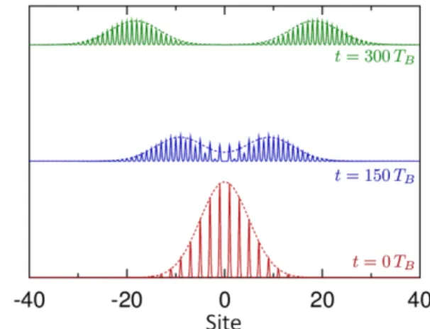
The dashed lines in Fig. 3 show the dynamical behav-ior of a massless particle (settingA0= 0in Eq. (13) leads
toE0 = 0) obtained from the above model [cf. Eq. (14)]
at time t = 0, 150TB and 300TB, where TB = 2π/F is the Bloch-period. The initial spinor (a+, a−) = (1,0)
withk0→0+, corresponds to a superposition of the
posi-tive energy eigenspinor(1, i)/√2and the negative energy eigenspinor(1,−i)/√2[cf. Eq. (18)] having opposite drift velocities±vD which from Eq. (17) read
vD= dω± dk k 0 = 2|Ω2cosk0| '2|Ω2|.
The comparison with the solution of exact Schrödinger equation (full lines) shows a very good agreement up to t= 300TB. One can verify that splitting into two sepa-rate wave packets moving with opposite group velocities ±vD which matches the expected theoretical value.
Figure 3. Evolution of an initial wave packet withk0 = 0,
σ = 10 and (a+, a−) = (1,0) [Eq. (20)] using the discrete
model given by Eq. (14) (dashed lines), at times t = 0
(red bottom line),150TB (blue middle line) and300TB (top green line) and compared to the exact Schrödinger equation simulation (full lines). Parameters are V1 = 6, F = 1,
¯
H(x, t) = 0.5 cos (πx) cos (ωBt)which givehϕg0|cos(πx)|ϕg1i=
−2.31×10⁻² (numerical value), andΩ2=−5.4×10⁻³. The
numerical value of the drift velocityvDagrees with the theo-retical valuevD= 2|Ω2cosk0|= 1.1×10⁻².
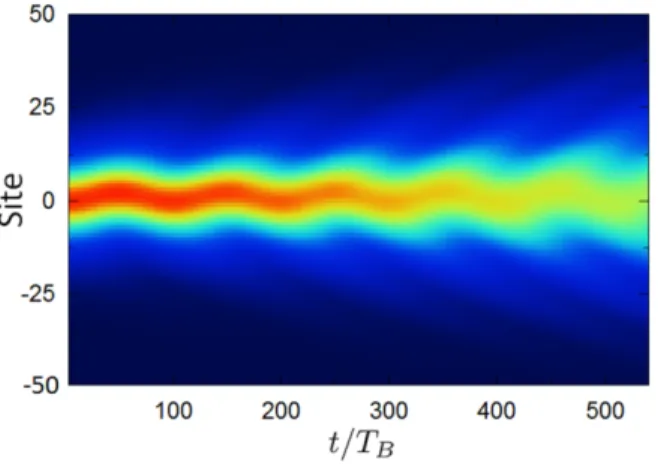
One of the most characteristic effects associated to the Dirac equation formassive particles is the so-called Zit-terbewegung (“trembling motion”), an interference effect between the positive and negative energy parts of the spinor resulting in a spatial jitter of the wave packet [46]. Such an effect was recently observed in quantum simu-lators of the Dirac equation with trapped ions [6], with ultracold atoms [47, 48], and in a photonic device [49, 50]. Figure 4 shows the spatio-temporal behavior of a wave packet for a massive particle governed by Eqs. (14), with a an initial spinor (a+, a−) = 2−1/2(1,1) and k0 = 0,
corresponding to superposition of positive and negative energy eigenstates (as can be seen from Eq. (16) in the limitk→0). In order to give a mass to the particle, we setA06= 0in Eq. (13), so thatE06= 0). We verified that
the same spatio-temporal behavior is obtained from the exact Schrödinger equation.
From Eq. (16) one can obtain the evolution of the wave packet’s average position
dhxi dt = 1 i~h[x, H]i=−2Ω2hσyi = 2iΩ2 ˆ dx c∗+(x, t)c−(x, t)−c.c. = 2iΩ2 ˆ dk ¯c∗+(k, t)¯c−(k, t)−c.c..
Figure 4. Zitterbewegung obtained from the discrete model Eq. (14) with initial spinor (a+, a−) = 2−1/2(1,1), σ = 10
and k0 = 0. The probability density is displayed in false
colors. Potential parameters are the same as in Fig. 3 except
¯
H(x, t) = cosπx(0.5 cosωBt+ 0.005). The time-independent contribution A0 = 0.005 in H¯ leads to a mass term E0 =
4.6×10⁻³.
momentum space) shows that the Zitterbewegung is due to the coherence between positive- and negative-energy states, confirming its physical interpretation as a quan-tum beat between odd- and even- site contributions (or positive and negative energy states in Dirac’s language). To the leading order ink≈0we find
dhxi dt = i2Ω2 √ 1−iDta ∗ +a−e2iE0t+ c.c (23)
withD= 4Ω22/(E0σ2). In this approximation, the
ampli-tude of the oscillation is seen to be directly proportional to the initial coherence a∗+a−. The oscillation has
fre-quency2E0, as it is the case for the electron’s
Zitterbe-wegung, and is slowly damped by diffusion effects with an effective coefficientD; note that the amplitude of the os-cillation forDt→0, is |Ω2|/E0= (2 ¯mc)−1, that is, half
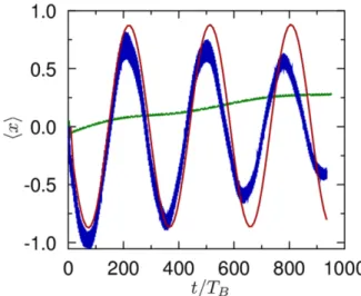
the dimensionless Compton wavelength, also in agree-ment with the Zitterbewegung of an electron. As shown in Fig. 5, the numerical calculations of hx(t)i from the exact Schrödinger equation and from the discrete model are in excellent agreement and match the theoretical am-plitude and period deduced from Eq. (23).
The effective parameters m=E0/4Ω22 andc = 2|Ω2|
can be calculated from the parameters used in the above simulations. For atoms of massM, they read, in dimen-sioned units, c = 2|Ω2|ERd/~= |Ω2| 2π2~/M λL and
m=E0ER/c2= E0/2π2Ω22
M. For cesium atoms and for potential parameters chosen in this section (E0 =
4.6×10⁻³,|Ω2| = 5.4×10⁻³) this leads to m∼9.3M
and c ∼ 1.33×10⁻⁴|Ω2|∼ 7×10⁻⁷m/s≈ 2×10⁻³vR,
wherevR=p2ER/M is the atom recoil velocity .
Figure 5. Evolution of the average positionhx(t)ifor0≤t≤
5TZB. Solid red line: Numerical result obtained from the ex-act Schrödinger equation. Blue circles: calculation from the discrete model Eq. (14). Same parameters as in Fig. 4. The Zitterbewegung period is in excellent agreement with the the-oretical value,TZB = 2π/(2E0) = 109TB, and its amplitude
with the prediction |Ω2|/E0 = 1.17. Due to diffusion, the
amplitude is attenuated by a factor(1 +D2t2)−1/2∼0.75at
t= 5TZB as compared to its initial value.
V. SPINOR-4 MODEL
We can also construct a full Dirac equation with a spinor-4. Using different coupling schemes we obtain ei-ther a Dirac-like equation in the standard representation or its analog in the Weyl representation. This beautifully illustrates the flexibility of the general model presented in Sec. III.
A. Spinor-4 Dirac representation
In order to construct a spinor-4 in the Dirac represen-tation, we consider both ground and excited WS ladders, nearest-neighbors inter-ladder couplings are set on and intra-ladder couplings are set off. The perturbation is thus of the form [cf. Eq. (6)]
¯
H =−V1f1(t) cos(2πx) +VS(x) with the modulation function
f1(t) =A (1) 1,1e iωBtei∆t+A(1) 1,−1e iωBte−i∆t+ c.c. From Eq. (9) we obtain the equations of motion
id dtcn =T gg n,0cn+T ge n,1dn+1+T ge n,−1dn−1 id dtdn =T ee n,0dn+T eg n,1cn+1+Tn,eg−1cn−1 with Tn,eg−1= Tn,ge1∗ , Tn,eg1= Tn,g,e−1∗ .
A Dirac-like equation is obtained if the coupling coefficients Tn,ge1 = −Tn,ge−1 are imaginary and if A(1)1,1hϕg0|cos(2πx)|ϕe 1i= −A (1) 1,−1hϕ g 1|cos(2πx)|ϕe0i, a
condition that is realized by tuning the modulation am-plitudes A(1)1,±1 so that they exactly compensate for the difference in the overlap integrals. The static pertur-bation VS(x) is chosen to be translation-invariant with respect to the reference lattice constant a = 1, so that Tn,gg0 =hϕg0|VS|ϕg0i ≡VSg and Tee
n,0 =hϕe0|VS|ϕe0i ≡VSe do not depend onn; the simple form used here isVS(x)∝
cos (4πx). Thus
id
dtcn=E0cn+iΩ1(dn+1−dn−1) id
dtdn=−E0dn+iΩ1(cn+1−cn−1) (24) where the couplingΩ1 is given by
iΩ1=Tn,ge1=−V1A (1) 1,1hϕ g 0|cos(2πx)|ϕ e 1i
(with A(1)1,1 imaginary) and the effective rest mass E0,
controlled by the static potentialVS(x),is given by [51]
E0=
VSg−Ve S
2 . (25)
The coupled equations (24) can be split into two in-dependent sub-lattices corresponding to sites cn with n even coupled to dn with n odd and conversely. Hence, we can build a 4-component Wannier-Stark spinor
ψ= c+ c− d+ d− (26)
where c±(x, t) and d±(x, t) are the slowly varying
en-velopes of cn and dn forn odd and n even respectively (in close analogy with what has been done in the spinor-2 case, Sec. IV and in App. A), giving
i∂tψ= (E0β−2Ω1αxpx)ψ (27)
which corresponds to the Dirac equation described by Eq. (2). As stated in Sec. II, this equation can be decou-pled into two equivalent sets
i∂ ∂t c+ d− = (E0σz−2Ω1pxσx) c+ d−
the other components(c−, d+)following exactly the same
equation. The corresponding dispersion relation is again ω±(k) = ± E02+ 4Ω21k2
1/2
, but each eigenvalue has now a double degeneracy. Note that this degeneracy can be lifted by adding other terms inH¯ (for instance, terms proportional to cos(πx) which break translation invari-ance with respect to the lattice step a= 1) and will be studied in a forthcoming paper.
The Zitterbewegung is described in the same way as for the spinor-2 case:
dhxi dt =−2Ω1hαxi =−2Ω1 ˆ dxc∗+(x, t)d−(x, t) + c.c +c∗−(x, t)d(x, t) + c.c. .
In the simple casepx = 0 with a spatially broad initial wave packetψ=2−1(a +, a−, b+, b−)G(k0)(x)one obtains dhxi dt =−2Ω1 a∗+b−+a∗−b+ e2iE0t+ c.c.
showing an oscillation amplitude proportional toΩ1/E0,
controlled by the initial coherence. The superposition of a “spin up particle” (a+, a−) and a “spin down
antipar-ticle” (b+, b−) ψ = 2−1(1,1,1,1) [52], leads to hx(t)i =
−(Ω1/E0) sin(2E0t). States with a∗+b−+a∗−b+
= 0, for instanceψ = 2−1(1,−1,1,1), display no Zitterbewe-gung. These results are illustrated in Fig. 6. The oscilla-tions (blue line) obtained from the Schrödinger equation are in good agreement with the simulation of Eq. (24) displayed in red. On the time scale of a few Zitterbe-wegung periodsTZB = 1/2E0, diffusion effects are here
negligible (one finds DTZB = 4Ω21π/(E02σ2) ∼ 10−2), but in contrast to the spinor-2 model displayed in Fig. 5, the exact Schrödinger equation shows parasitic Landau-Zener tunneling into the continuum (due to the presence of populated excited states d±), leading to a slow
de-crease in the spinor negative-energy amplitudes and thus to the oscillation amplitude. Fast, small-amplitude Rabi oscillations at frequencyΩ1TZB−1 between ground and
excited states are responsible for the apparent thickening of the blue line in Fig. 6: it is due to the asymmetry of the excited stateϕen(x)with respect to the center of its welln leading thus an average position which differs by a fraction of a lattice step as compared to the ground state average position. Note finally that the second ini-tial condition spinorψ= 2−1(1,−1,1,1)(green line) do
not display Zitterbewegung, as expected.
B. Spinor-4 Weyl representation
A Dirac equation in the Weyl representation can be obtained with a different coupling scheme. The calcula-tion follows the same lines as in the previous seccalcula-tion, and we shall simply indicate the main steps below. We use the HamiltonianH¯ of Eq. (6) with VS(x) = 0and with the modulations f2(t) =A (2) 1,1e iωBtei∆t+A(2) 1,−1e iωBte−i∆t+ c.c. f1(t) =A (1) 0,1e i∆t+ c.c.
Figure 6. Evolution of the average position hx(t)i for0 ≤
t ≤ 3TZB. Exact Schrödinger equation (thick blue line) and discrete model Eq. (24) (red line) for an initial spinor
2−1(1,1,1,1),σ2 = 500andk0= 0. The non-oscillating green
line is the exact Schrödinger equation result for an initial spinor2−1(1,−1,1,1), which does not show Zitterbewegung.
Potential parameters areV1 = 6,F = 1,A(1)1,1=−5.0×10
−3
i
and A(1)1,−1 =−7.5×10
−3
i giving Ω1 = −1.5×10⁻³. The
effective mass E0 = 1.6×10⁻³ is generated by the
poten-tial VS(x) = 5×10⁻³cos(4πx). The Zitterbewegung pe-riod and amplitude agree with the theoretical valuesTZB = 2π/(2E0) = 310TB and|Ω1|/E0= 0.93.
The general developments of Sec. III then lead to:
id dtcn=T ge n,1dn+1+T ge n,−1dn−1+T ge n,0dn id dtdn=T eg n,1cn+1+Tn,eg−1cn−1+Tn,eg0cn.
We then chooseA(1)0,1 real and define the real parameter EW =Tn,ge0=Tn,eg0 =−A(1)0,1V1hϕ g 0|cos(2πx)|ϕ e 0i.
Making the amplitudes A(2)1,±1 imaginary and tun-ing them in such a way that A(2)1,1hϕg0|cos(πx)|ϕe
1i=
A(2)−1,1hϕ1g|cos(πx)|ϕe0i, one has
Tn,ge1= (−1)nV2A (2) 1,1hϕ g 0|cos(πx)|ϕ e 1i=i(−1) nΩ W Tn,ge−1= (−1)nV2A (2) −1,1hϕ g 0|cos(πx) ϕe−1 =−i(−1)nΩW Tn,eg1=Tn,ge1 Tn,eg−1=−Tn,ge1 and thus id dtcn= (−1) n iΩ W(dn+1−dn−1) +EWdn id dtdn=−(−1) niΩ W(cn+1−cn−1) +EWcn. (28)
The continuous limit of these two equations gives
i∂tc+(x, t) =−2ΩWpxd−+EWd+
i∂td−(x, t) =−2ΩWpxc++EWc−
i∂td+(x, t) = 2ΩWpxc−+EWc+
i∂tc−(x, t) = 2ΩWpxd++EWd−.
The Weyl spinor-4 is thus defined as ψW(x, t) = (c+, d−, d+, c−) and follows the equation i∂tψW = HWψW with HW =−2ΩW σxpx 0 0 −σxpx +EW 0 1 1 0
which is the Dirac Hamiltonian in the Weyl representa-tion, Eq. (4), withpparallel to thexaxis.
VI. PROSPECTS FOR AN EXPERIMENTAL
REALIZATION
The present proposal of a quantum simulator of Dirac physics depends on techniques that are widely used ex-perimentally. It is based on driving of ultracold atoms by modulations of a 1D optical lattice [36, 53], a technique that has been used from the early days of optical lattice physics, from the seminal experiments of observation of Bloch oscillations [29] and the Wannier-Stark ladder [30], dynamical localization and Anderson physics [54, 55], Landau-Zener tunneling [41, 56], to, more recently, the generation of artificial gauge fields [11, 57]. This makes our system particularly simple, both conceptually and experimentally, not involving, for example, Raman tran-sitions or Zeeman-level manipulation. The main limita-tion of driven systems is the loss of atoms to the contin-uum via dynamic Landau-Zener coupling, which requires a careful optimization of the parameters. However, most effects described here survive to moderate losses, e.g. the Zitterbewegung, as it can be seen from Figs. 4 and 6.
Several techniques have also been developed for atom detection, recently attaining single-site resolution thanks to thequantum gas microscope[58, 59] or near-field imag-ing [60]. For the particular situation studied here, a possible difficulty is the necessity of distinguishing the contribution of atoms located in even and odd sites. This can obviously be done site by site if single-site resolution is attained. Another, potentially more prac-tical, way to do so is to select atoms from even/odd sitesbefore detection. A possible strategy is the follow-ing: After the desired dynamics is studied (e.g. Zit-terbewegung) the tilt of the potential is adiabatically tuned to zero, leaving only a flat trapping potential Vacos(2kLx) exp(−y2/w2
a), where we take into account the tranverse Gaussian profile of the laser beam. One then turns on adiabatically a transversely-shifted double-period potentialVbcos(kLx+ϕ) exp−(y−y0)2/w2b
; for ϕ = 0 (resp. π) this potential will mostly affect even (resp. odd) sites. By adjusting the ratioVb/Va and the
shifty0 one can create a transverse “gutter” that induces
losses in even (resp. odd) sites. One can then either de-tect the lost atoms, that is even- (resp. odd-)site popu-lation, or remaining atoms, i.e. odd- (resp. even-) site population. If the potential allows two Wannier-Stark ladders, one can adjustVa before turningVb on so as to induce losses in the excited WS ladder.
As a concrete example, consider the 4-spinor ψ = (c+, c−, d+, d−)Eq. (26). In the particle-antiparticle
con-text, the first component c+ (for example) corresponds
to the spin-up component for a particle at rest. In our quantum simulator it corresponds to the slowly vary-ing envelope of the population of the ground ladder odd sites. Such quantity can be measured by first lowering the potential barrier (or increasing the slope) so that the atoms in the excited ladder escape, and then measuring the population |c+(x)|
2
using the techniques described above. For the excited ladder components as |d+(x)|2
(odd sites), one can first remove even-site atoms using the method presented above, then lower the lattice depth al-lowing the excited-ladder atoms to escape while ground-ladder atoms remain trapped, and one detects the atoms that are leaking. The other components can be detected in a similar way.
VII. CONCLUSION
The present work introduces a general scheme based on the Wannier-Stark Hamiltonian, realizable with ultracold atoms in 1D optical lattices, allowing for the quantum simulation of Dirac physics, with a great flexibility in the choice of the parameters and of the properties of the re-sulting quantum simulator. One can control the effective mass, realize spinor-2 and spinor-4 Dirac equations both in the standard and in the Weyl representation. Our general model opens a large field of other possibilities which will be developed in forthcoming papers. For in-stance, the spinor-4 obtained as two degenerate spinor-2 systems can be studied in the case where the degeneracy is lifted, leading to flat bands or to spin3/2-like relativis-tic parrelativis-ticles. The possibilities are even more exciting if one generalizes the above approach to higher dimensions. In dimension 2, one can use lattice temporal modula-tions to generate non-trivial artificial gauge fields [5, 19], and quantum simulate the Dirac particle interaction with electromagnetic fields (e.g. simulate the “gyromagnetic factor” of our “artificial electron”). If one uses interact-ing bosonic atoms in the mean-field limit described by the Gross-Pitaevskii equation, we can study Dirac physics in the presence of a nonlinearity, which can lead to quasi-classical “relativistic” chaos [61]. All these possibilities put into evidence the power of ultracold atoms and opti-cal potentials as quantum simulator for a rich variety of physical systems.
ACKNOWLEDGMENTS
This work is supported by Agence Nationale de la Recherche (Grant K-BEC No. ANR-13-BS04-0001-01), the Labex CEMPI (Grant No. ANR-11-LABX-0007-01), as well as by the Ministry of Higher Education and Re-search, Hauts de France council and European Regional Development Fund (ERDF) through the Contrat de Pro-jets Etat-Region (CPER Photonics for Society, P4S).
Appendix A: Detailed derivation of the Dirac Hamiltonian
This Appendix presents in more detail the calculation leading to the coupled equations of Eqs. (7), and show how a a Dirac-like Hamiltonian can be obtained.
We consider here the wave packet of Eq. (5) and project the Schrodinger equation,idΨ/dt= (H0+ ¯H)Ψ on the
WS states [noting thatcn=hϕg
n|Ψiexp (iωBt)anddn = hϕe n |Ψiexp (iωBt+i∆t)]: id dtcn = X r∈Z hϕg n|H¯ ϕ g n+r e−irωBtc n+r +hϕg n|H¯ ϕen+r e−irωBte−i∆tdn +r id dtdn = X r∈Z hϕen|H¯ ϕ g n+r e−irωBtc n+r +hϕe n|H¯ ϕen+r e−irωBte−i∆tdn +r (A1) where the “free evolution” due toH0 is canceled out. In
the following, we take as an example the particular per-turbation ¯ H(t) =−V1cos(2πx)f1(t) (A2) with f1(t) =A (1) 1,1e iωBtei∆t+A(1) 1,−1e iωBte−i∆t+ c.c. (A3)
The results for any other choice of Hamiltonian can be obtained along the same lines.
From Eqs. (A1), we then have:
id dtcn=−V1 X r∈Z hϕg n|cos 2πx ϕ g n+r f1(t)e−irωBtcn+r +hϕgn|cos 2πx ϕen+r f1(t)e−irωBte−i∆tdn+r id dtdn=−V1 X r∈Z hϕe n|cos 2πx ϕ g n+r f1(t)e−irωBtei∆tcn+r +hϕen|cos 2πx ϕen+r f1(t)e−irωBtdn+r . (A4)
We now introduce two simplifying assumptions: (i) The overlap integrals between WS states rapidly shrink to zero for |r| > 1 and we can thus consider only nearest neighbor couplings, and (ii) we neglect fast oscillations
and keep only resonant contributions in Eq. (A4), which eliminates intra-ladder couplings (assuming that∆is far fromωB). We obtain: id dtcn=−V1A (1) 1,1hϕ g 0|cos 2πx|ϕ e 1idn+1 −V1A (1)∗ 1,−1hϕ g 0|cos 2πx ϕ e −1 dn−1 id dtdn=−V1A (1) 1,−1hϕ e 0|cos 2πx|ϕ g 1icn+1 −V1A (1)∗ 1,1 hϕ e 0|cos 2πx ϕ g −1 cn−1, (A5)
that is, Eq. (9) with intra-ladder couplings off and the inter-ladder couplings of Eq.(11). In Eq. (A5), we took into account the reality condition off1(t),A
(1)∗
1,−1=A (1)
−1,1,
A(1)1,1∗=A(1)−1,−1, and the properties of overlap integrals:
hϕgn|cos 2πx ϕ e n±1 = ˆ ϕgn(x)ϕne±1(x) cos(2πx)dx = ˆ ϕg0(x−n)ϕ±e1(x−n) cos(2πx)dx =hϕg0|cos 2πxϕe±1 and hϕen|cos 2πx ϕ g n±1 =hϕe0|cos 2πx ϕ g ±1 =hϕg0|cos 2πx ϕe∓1
where the translational invariance of WS states was used. In the general framework of Sec. III, other contribu-tions to the coupling coefficients may have to be consid-ered in Eqs. (10) and (11), and can be obtained in the same way. Note that if a perturbation component pro-portional tocos(πx)is present, the overlap integrals are
hϕg n|cosπx ϕen±1 = ˆ ϕgn(x)ϕne±1(x) cos(πx)dx = ˆ ϕg0(x)ϕe±1(x) cos(πx+πn)dx = (−1)nhϕg0|cosπxϕe±1 hϕe n|cosπx ϕ g n±1 =±(−1)nhϕe 0|cosπx ϕ g ±1 , and thus depend on the even or odd character of the site labeln.
A Dirac-like equation can be derived from Eq. (A5). If we tune the modulation coefficients such that
A(1)1,1hϕg0|cos 2πx|ϕe 1i=−A (1)∗ 1,−1hϕ g 0|cos 2πx ϕe−1 we find id dtcn=−V1A (1) 1,1hϕ g 0|cos 2πx|ϕ e 1i[dn+1−dn−1], id dtdn=A (1)∗ 1,1 V1hϕe1|cos 2πx|ϕ g 0i[cn+1−cn−1]
and assuming imaginary amplitudes (i.e choosing the phase of the modulations suitably) gives
id dtcn=iΩ [dn+1−dn−1] id dtdn=iΩ [cn+1−cn−1] (A6) where, V1A (1) 1,1hϕ g
0|cos 2πx|ϕe1i =−iΩ. Note that these
equations correspond to two independent sub-lattices, the amplitudes cn for n odd being coupled to dn for n even, and conversely.
We thus conclude that the “suitable” form of the po-tential corresponding to Eqs. (A2) and (A3) leading to Eq. (A6) is f1(t) = 2a (1) 1,1sin (ωBt+ ∆t) + 2a (1) 1,−1sin (ωBt−∆)
where a1,±1 = −iA1,±1 are real amplitudes with
relative weight obeying a(1)1,1hϕg0|cos 2πx|ϕe
1i= a1,−1hϕ g 0|cos 2πx ϕe−1 .
We can take the continuous limit of these equations assuming that the amplitudescn, dn are slowly varying at the scale of the lattice step. We can then introduce the smooth envelopes associated to each sub-lattice: cn(t) = c±(x=n, t)(the sign±corresponding tonodd or even)
anddn(t) =d±(x=n, t). We then get
i∂tc±=i2Ω ∂d∓(x, t) ∂x i∂td±=i2Ω ∂c∓(x, t) ∂x
This last expression written as a Dirac equation for a massless particle corresponding to Eq. (27) withE0= 0.
[1] I. M. Georgescu, S. Ashhab, and F. Nori, “Quantum simulation,” Rev. Mod. Phys.86, 153–185 (2014). [2] I. Bloch, J. Dalibard, and S. Nascimbene, “Quantum
simulations with ultracold quantum gases,” Nat. Phys. 8, 267–276 (2014).
[3] R. P. Feynman, “Simulating Physics with Computers,” Int. J. Theor. Phys.21, 467–488 (1982).
[4] I. Bloch, J. Dalibard, and W. Zwerger, “Many-body physics with ultracold gases,” Rev. Mod. Phys.80, 885–
964 (2008).
[5] J. Dalibard, F. Gerbier, G. Juzeli¯unas, and P. Öhberg, “Artificial gauge potentials for neutral atoms,” Rev. Mod. Phys.83, 1523–1543 (2011).
[6] R. Gerritsma, G. Kirchmair, F. Zahringer, E. Solano, R. Blatt, and C. F. Roos, “Quantum simulation of the Dirac equation,” Nature (London)463, 68–71 (2010). [7] D. Witthaut, T. Salger, S. Kling, C. Grossert, and
in bichromatic optical lattices,” Phys. Rev. A84, 033601 (2011).
[8] T. Salger, C. Grossert, S. Kling, and M. Weitz, “Klein Tunneling of a Quasirelativistic Bose-Einstein Conden-sate in an Optical Lattice,” Phys. Rev. Lett.107, 240401 (2011).
[9] V. Galitski and I. B. Spielman, “Spin-orbit coupling in quantum gases,” Nature (London)494, 49–54 (2013). [10] Y.-J. Lin, R. L. Compton, K. Jimenez-Garcia, J. V.
Porto, and I. B. Spielman, “Synthetic magnetic fields for ultracold neutral atoms,” Nature (London)462, 628– 632 (2009).
[11] J. Struck, C. Ölschläger, M. Weinberg, P. Hauke, J. Si-monet, A. Eckardt, M. Lewenstein, K. Sengstock, and P. Windpassinger, “Tunable Gauge Potential for Neutral and Spinless Particles in Driven Optical Lattices,” Phys. Rev. Lett. 108, 225304 (2012).
[12] J. Chabé, G. Lemarié, B. Grémaud, D. Delande, P. Szrift-giser, and J. C. Garreau, “Experimental Observation of the Anderson Metal-Insulator Transition with Atomic Matter Waves,” Phys. Rev. Lett.101, 255702 (2008). [13] J. Billy, V. Josse, Z. Zuo, A. Bernard, B. Hambrecht,
P. Lugan, D. Clément, L. Sanchez-Palencia, P. Bouyer, and A. Aspect, “Direct observation of Anderson local-ization of matter-waves in a controlled disorder,” Nature (London)453, 891–894 (2008).
[14] G. Roati, C. d’Errico, L. Fallani, M. Fattori, C. Fort, M. Zaccanti, G. Modugno, M. Modugno, and M. In-guscio, “Anderson localization of a non-interacting Bose-Einstein condensate,” Nature (London) 453, 895–898 (2008).
[15] S. S. Kondov, W. R. McGehee, J. J. Zirbel, and B. De-Marco, “Three-Dimensional Anderson Localization of Ul-tracold Matter,” Science334, 66–68 (2011).
[16] I. Manai, J.-F. Clément, R. Chicireanu, C. Hainaut, J. C. Garreau, P. Szriftgiser, and D. Delande, “Experimental Observation of Two-Dimensional Anderson Localization with the Atomic Kicked Rotor,” Phys. Rev. Lett. 115, 240603 (2015).
[17] S. Wang, B.-C. Lin, A.-Q. Wang, D.-P. Yu, and Z.-M. Liao, “Quantum transport in Dirac and Weyl semimetals: a review,” Advances in Physics: X2, 518–544 (2017). [18] A. A. Soluyanov, D. Gresch, Z. Wang, Q. Wu, M. Troyer,
X. Dai, and B. A. Bernevig, “Type-II Weyl semimetals,” Nature (London)527, 495–498 (2017).
[19] L. Lamata, J. Casanova, R. Gerritsma, C. F. Roos, J. J. García-Ripoll, and E. Solano, “Relativistic quantum me-chanics with trapped ions,” New J. Phys 13, 095003 (2011).
[20] R. Gerritsma, B. P. Lanyon, G. Kirchmair, F. Zähringer, C. Hempel, J. Casanova, J. J. García-Ripoll, E. Solano, R. Blatt, and C. F. Roos, “Quantum Simulation of the Klein Paradox with Trapped Ions,” Phys. Rev. Lett.106, 060503 (2011).
[21] D. Suchet, M. Rabinovic, T. Reimann, N. Kretschmar, F. Sievers, C. Salomon, J. Lau, O. Goulko, C. Lobo, and F. Chevy, “Analog simulation of Weyl particles with cold atoms,” EPL (Europhysics Letters)114, 26005 (2016). [22] L. Mazza, A. Bermudez, N. Goldman, M. Rizzi, M. A.
Martin-Delgado, and M. Lewenstein, “An optical-lattice-based quantum simulator for relativistic field theories and topological insulators,” New J. Phys 14, 015007 (2012).
[23] A. R. Kolovsky and E. N. Bulgakov, “Wannier-Stark
states and Bloch oscillations in the honeycomb lattice,” Phys. Rev. A87, 033602 (2013).
[24] L. Tarruell, D. Greif, T. Uehlinger, G. Jotzu, and T. Esslinger, “Creating, moving and merging Dirac points with a Fermi gas in a tunable honeycomb lattice,” Nature (London)483, 302–305 (2012).
[25] X. Lopez-Gonzalez, J. Sisti, G. Pettini, and M. Mod-ugno, “Effective Dirac equation for ultracold atoms in optical lattices: Role of the localization properties of the Wannier functions,” Phys. Rev. A89, 033608 (2014). [26] K. Jiménez-García, L. J. LeBlanc, R. A. Williams, M. C.
Beeler, C. Qu, M. Gong, C. Zhang, and I. B. Spiel-man, “Tunable Spin-Orbit Coupling via Strong Driving in Ultracold-Atom Systems,” Phys. Rev. Lett.114, 125301 (2015).
[27] D.-W. Zhang, Z.-D. Wang, and S.-L. Zhu, “Relativistic quantum effects of Dirac particles simulated by ultracold atoms,” Front. Phys.7, 31–53 (2012).
[28] A. R. Kolovsky, “Simulating cyclotron-Bloch dynamics of a charged particle in a 2D lattice by means of cold atoms in driven quasi-1D optical lattices,” Front. Phys. 7, 3 (2012).
[29] M. Ben Dahan, E. Peik, J. Reichel, Y. Castin, and C. Sa-lomon, “Bloch Oscillations of Atoms in an Optical Poten-tial,” Phys. Rev. Lett.76, 4508–4511 (1996).
[30] Q. Niu, X. G. Zhao, G. A. Georgakis, and M. G. Raizen, “Atomic Landau-Zener Tunneling and Wannier-Stark Ladders in Optical Potentials,” Phys. Rev. Lett. 76, 4504–4507 (1996).
[31] A. R. Kolovsky, E. A. Gómez, and H. J. Korsch, “Bose-Einstein condensates on tilted lattices: Coherent, chaotic, and subdiffusive dynamics,” Phys. Rev. A 81, 025603 (2010).
[32] A. R. Kolovsky, H. J. Korsch, and E.-M. Graefe, “Bloch oscillations of Bose-Einstein condensates: Quan-tum counterpart of dynamical instability,” Phys. Rev. A 80, 023617 (2009).
[33] M. Glück, A. R. Kolovsky, and H. J. Korsch, “Fractal stabilization of Wannier-Stark resonances,” EPL (Euro-physics Letters)51, 255–260 (2000).
[34] M. Glück, A. R. Kolovsky, and H. J. Korsch, “Lifetime of Wannier-Stark states,” Phys. Rev. Lett. 83, 891–894 (1999).
[35] M. Glück, A. R. Kolovsky, and H. J. Korsch, “Wannier-Stark resonances in optical and semiconductor superlat-tices,” Phys. Rep.366, 103–182 (2002).
[36] C. Cohen-Tannoudji and D. Guéry-Odelin,Advances In Atomic Physics: An Overview (World Scientific Publish-ing, Singapore, 2011).
[37] Q. Thommen, J. C. Garreau, and V. Zehnlé, “Theo-retical analysis of quantum dynamics in one-dimensional lattices: Wannier-Stark description,” Phys. Rev. A 65, 053406 (2002).
[38] G. Nenciu, “Dynamics of band electrons in electric and magnetic fields: rigorous justification of the effective Hamiltonians,” Rev. Mod. Phys.63, 91–127 (1991). [39] Technically speaking, in infinite space, WS states are
“resonances” – metastable states [38], but for our present purposes they can be considered as stationary states as long as the duration of the experiment is much shorter than their lifetime. We checked numerically the validity of this hypothesis throughout this work.
[40] Q. Thommen, J. C. Garreau, and V. Zehnlé, “Quan-tum motor: Directed wave-packet motion in an optical
lattice,” Phys. Rev. A84, 043403 (2011).
[41] A. Zenesini, H. Lignier, G. Tayebirad, J. Radogostowicz, D. Ciampini, R. Mannella, S. Wimberger, O. Morsch, and E. Arimondo, “Time-Resolved Measurement of Landau-Zener Tunneling in Periodic Potentials,” Phys. Rev. Lett. 103, 090403 (2009).
[42] N. Goldman, J. Dalibard, M. Aidelsburger, and N. R. Cooper, “Periodically driven quantum matter: The case of resonant modulations,” Phys. Rev. A 91, 033632 (2015).
[43] P. A. M. Dirac, “The Quantum Theory of the Electron,” Proc. Royal Soc. London A117, 610–624 (1928). [44] P. B. Pal, “Dirac, Majorana, and Weyl fermions,” Am. J.
Phys.79, 485–498 (2011).
[45] Experimentally this can be done by trapping the atoms on a shallow optical lattice and increasing adiabatically the lattice amplitude to the desired level.
[46] J. Y. Vaishnav and C. W. Clark, “Observing Zitterbe-wegung with Ultracold Atoms,” Phys. Rev. Lett. 100, 153002 (2008).
[47] L. J. LeBlanc, M. C. Beeler, K. Jiménez-García, A. R. Perry, S. Sugawa, R. A. Williams, and I. B. Spielman, “Direct observation of zitterbewegung in a Bose–Einstein condensate,” New J. Phys15, 073011 (2013).
[48] C. Qu, C. Hamner, M. Gong, C. Zhang, and P. Engels, “Observation of Zitterbewegung in a spin-orbit-coupled Bose-Einstein condensate,” Phys. Rev. A 88, 021604 (2013).
[49] F. Dreisow, M. Heinrich, R. Keil, A. Tünnermann, S. Nolte, S. Longhi, and A. Szameit, “Classical Simula-tion of Relativistic Zitterbewegung in Photonic Lattices,” Phys. Rev. Lett.105, 143902 (2010).
[50] S. Longhi, “Photonic analog of Zitterbewegung in binary waveguide arrays,” Opt. Lett.35, 235–237 (2010).
[51] We simply redefined (cn, dn) as
(cn, dn) exp [−i(VSg+VSe)t/2].
[52] This distinction is meaningful only ifpmc.
[53] A. Eckardt, “Atomic quantum gases in periodically driven optical lattices,” Rev. Mod. Phys. 89, 011004 (2017).
[54] F. L. Moore, J. C. Robinson, C. Bharucha, P. E. Williams, and M. G. Raizen, “Observation of Dynam-ical Localization in Atomic Momentum Transfer: A New Testing Ground for Quantum Chaos,” Phys. Rev. Lett. 73, 2974–2977 (1994).
[55] J. C. Garreau, “Quantum simulation of disordered sys-tems with cold atoms,” Compt. Rendus Phys.18, 31 – 46 (2017).
[56] C. E. Creffield, F. Sols, D. Ciampini, O. Morsch, and E. Arimondo, “Expansion of matter waves in static and driven periodic potentials,” Phys. Rev. A 82, 035601 (2010).
[57] P. Hauke, O. Tieleman, A. Celi, C. Ölschläger, J. Si-monet, J. Struck, M. Weinberg, P. Windpassinger, K. Sengstock, M. Lewenstein, and A. Eckardt, “Non-Abelian Gauge Fields and Topological Insulators in Shaken Optical Lattices,” Phys. Rev. Lett.109, 145301 (2012).
[58] D. Greif, M. F. Parsons, A. Mazurenko, C. S. Chiu, S. Blatt, F. Huber, G. Ji, and M. Greiner, “Site-resolved imaging of a fermionic Mott insulator,” Science351, 953– 957 (2016).
[59] E. Haller, J. Hudson, A. Kelly, D. A. Cotta, B. Peaude-cerf, G. D. Bruce, and S. Kuhr, “Single-atom imaging of fermions in a quantum-gas microscope,” Nat. Phys.11, 738–742 (2017).
[60] B. Zimmermann, T. Müller, J. Meineke, T. Esslinger, and H. Moritz, “High-resolution imaging of ultracold fermions in microscopically tailored optical potentials,” New J. Phys13, 043007 (2011).
[61] Q. Thommen, J. C. Garreau, and V. Zehnlé, “Classical Chaos with Bose-Einstein Condensates in Tilted Optical Lattices,” Phys. Rev. Lett.91, 210405 (2003).